arXiv:quant-ph/0702123v2 14 Feb 2007
Simon J. Devitt,1, 2 Sonia G. Schirmer,1 Daniel K. L. Oi,1, 3 Jared H. Cole,2and Lloyd C.L. Hollenberg2
1
Centre for Quantum Computation, Department of Applied Mathematics and Theoretical Physics, University of Cambridge, Wilberforce Road, Cambridge CB3 0WA, United Kingdom
2
Centre for Quantum Computing Technology, Department of Physics, University of Melbourne, Victoria, Australia∗ 3
SUPA, Department of Physics, University of Strathclyde, Glasgow G4 0NG, United Kingdom
The basic operating element of standard quantum computation is the qubit, an isolated two-level system that can be accurately controlled, initialized and measured. However, the majority of proposed physical architectures for quantum computation are built from systems that contain much more complicated Hilbert space structures. Hence, defining a qubit requires the identification of an appropriate controllable two-dimensional sub-system. This prompts the obvious question of how well a qubit, thus defined, is confined to this subspace, and whether we can experimentally quantify the potential leakage into to states outside the qubit subspace. In this paper we demonstrate that subspace leakage can be quantitatively characterized using minimal theoretical assumptions by examining the Fourier spectrum of the Rabi oscillation experiment.
PACS numbers: 03.67.Lx, 03.65.Wj
I. INTRODUCTION
The issue of subspace confinement for qubit systems is fundamental to the primary operating assumptions of quantum processors. The concepts of universality, quan-tum gate operations, algorithms, error correction and fault-tolerant computation hinge on the precept that the fundamental quantum system is an isolated, controllable, two-dimensional system (qubit).
It is well known that most of the physical realiza-tions of qubits are in fact multi-level quantum systems, which can theoretically be confined to a two-dimensional (qubit) subspace. Important examples range from super-conducting qubits [1, 2, 3] to atomic systems such as cavity-coupled color centers [4, 5, 6] and ion traps [7]. In the former systems, a qubit is generally defined as the subspace (of the full Hilbert space) spanned by the two lowest energy states in an arbitrarily shaped potential such as the washboard potential of current-biased Josephson Junctions [8, 9]. However, the poten-tial number of valid quantum states within each well is not limited to two, and quantum gates, especially if sub-optimally implemented, may inadvertently populate these states. Similarly in ion trap systems, a qubit is usually defined by two electronic states of an ion, either two hyperfine levels or a ground state and a meta-stable excited state, but once again there exist many other elec-tronic states. Hence a more stringent definition of a qubit would consist of a two-level quantum system with classi-cal control confined to the unitary groupSU(2).
The ability to initialize, operate and measure com-pletely within the two-level subspace representing “the qubit” is vital to the successful operation of any large scale device constructed from such quantum systems. Standard quantum error correction protocols (QEC) [10,
∗Electronic address: [email protected]
11, 12] generally assume that the qubit system is precisely confined to the two-level subspace and that all quantum gates operate only on the qubit degrees of freedom. If poor control or environmental influences inadvertently result in non-zero population of higher levels then error correction protocols that can correct leakage errors are necessary.
The issue of subspace leakage in quantum processing has been addressed in depth from the standpoint of error correction. Work by Lidar [13, 14] examined the con-struction of Leakage Reduction Units (LRU’s), which use modified pulsing techniques to ensure that any unitary dynamics outside the qubit subspace can be compen-sated for which has been adapted specifically for super-conducting systems [15]. Another type of LRU’s uses quantum teleportation [16] to map a multi-level quantum state back to a freshly initialized two-level qubit. Finally, active detection such as non-demolition measurements (which detect population in non-qubit states without dis-criminating between the qubit states) can be performed on the system [17, 18, 19, 20]. If an out-of-subspace de-tection event occurs the leaked qubit is re-initialized or replaced. The inclusion of LRU’s based on teleportation has been investigated within the context of fault-tolerant quantum computation [21] and shows that, in principle, the inclusion of leakage protection does not adversely af-fect large scale concatenated error correction.
schemes in many cases, provided that we can experimen-tally ascertain sufficiently high confinement of manufac-tured qubits under classically controlled Hamiltonian dy-namics.
In this paper we present a simple generic protocol to estimate qubit confinement, or more precisely, establish bounds on the subspace leakage rates, for “quality con-trol” purposes. The main goal is to allow us to empir-ically detect inferior qubits by using readily obtainable experimental data to derive tight bounds on the subspace leakage of the system. This protocol would represent one of the first steps towards full system characterization pro-tocols [22, 23, 24, 25].
Section II briefly outlines the basic assumptions with respect to the measurement and control model and the motivation for the proposed protocol. Section III dis-cusses the basic mathematical properties of Rabi oscil-lation data and shows how a minimal amount of infor-mation obtained from the Rabi spectrum can be used to derive empirical bounds on the subspace leakage rate, and that these bounds are very tight for the high qual-ity qubits required for practical quantum computation. In section IV, the effects of finite sampling are consid-ered and studied using numerical simulations. Section V
compares the efficiency of bounding confinement using the proposed scheme versus alternative approaches such as detection of imperfect confinement by identifying ad-ditional transition peaks within the Rabi spectrum. Fi-nally, section VI briefly examines the effects of decoher-ence on the protocol.
II. MOTIVATION AND PRELIMINARIES
Estimation of qubit confinement represents one of the first major steps in full qubit characterization. Therefore, the protocol should not be predicated on the availabil-ity of sophisticated measurements or control, and should be amenable to automation so that it could be used in conjunction with a potentially automated qubit manu-facturing process. The bounds on the subspace leakage will be based on the observable qubit evolution under an externally controlled driving Hamiltonian. We assume that the induced Hamiltonian dynamics is piecewise con-stant in time and therefore induces the unitary operator
[image:2.612.83.518.348.538.2]U =e−iHt, with~= 1.
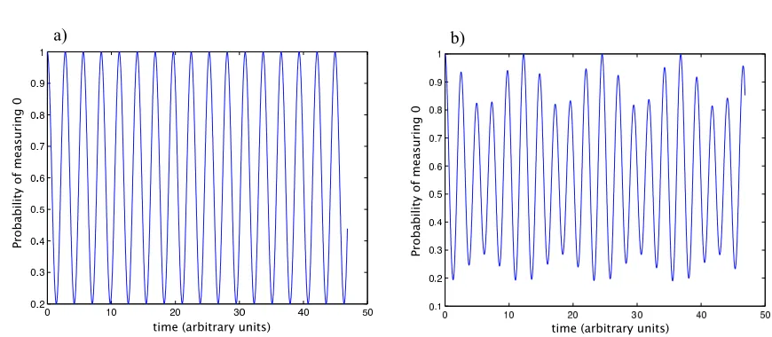
FIG. 1: Modulations in the Rabi oscillations of a three-level system driven by the Hamiltonian, a) Eq. 2 and b) Eq. 1. Fig. b) provides clear evidence that this system is not a qubit, while Fig. a) appears to show perfect confinement. However the analysis in the following sections will show that the subspace confinement for this system (h0+ 2h0,1 = 0.9992) is in fact not sufficient for large-scale QIP applications.
The measurement model assumed is crucial to the rele-vance of the protocol. Some standard measurement mod-els in quantum computation assume the ability to de-tect both the |0i and |1i states independently (such as SET detectors in solid state designs [26, 27, 28]). In this case, estimating subspace leakage is fairly straight-forward and requires only repeated measurement of the system while undergoing evolution. The leakage is
can leak to an external detection circuit. The measure-ment outcome of the indirectly probed state is inferred from the non-detection of the directly measured state and for such measurement models estimating confinement is more complicated. Hence this paper utilizes the latter model in order to quantify confinement. It should be noted that we are not considering the concept of weak measurement, in each case we assume that the measure-ment of the system causes a full POVM collapse of the wavefunction.
Strong non-qubit transitions can still be identified di-rectly via modulations in the Rabi oscillations data as shown in Fig. 1b for a three-state system evolving under the trial Hamiltonian
Hm=
0 1 0.5 1 1 0 0.5 0 1.5
. (1)
However, the Rabi oscillation data for the modified three-state Hamiltonian,
Hn =
0 1 0.01
1 1 0
0.01 0 1.5
, (2)
depicted in Fig. 1a shows that an apparent lack of modu-lations in the Rabi oscillation data is not proof of perfect confinement, and that quantitative measures of confine-ment or subspace leakage and expericonfine-mental protocols are needed.
III. ESTIMATION OF SUBSPACE LEAKAGE
By defining the projection operator onto a two dimen-sional subspace, Π =|0ih0|+|1ih1|, subspace leakage is given by,
ǫ= 1−Tr[Πρ], (3)
withρ=U†(t)|0ih0|U(t). Unfortunately, we cannot
cal-culateǫ directly without knowledge of the Hamiltonian. However, we can estimate subspace leakage experimen-tally from standard Rabi oscillation data.
A. Perfect confinement
Consider a general N-level system undergoing coher-ent evolution via a driving HamiltonianHN in the closed
system case of no environmental decoherence. If confine-ment under this Hamiltonian is perfect,HN has a direct
sum decomposition,
HN =H2×2⊕H(N−2)×(N−2) (4) whereH2×2represents the control Hamiltonian confined to the qubit subspace, span{|0i,|1i}, the state|0ibeing
defined by the measurement, and the excited state |1i
by the allowed transition. For our measurement model the observed Rabi oscillations have the functional form
f(t) =|h0|UN(t)|0i|2. As there is no coupling between
the state |0i and states outside the H2×2 subspace, we can expandf(t) by diagonalizingU2= exp(−iH2×2t)
f(t) =|h0|A†diag{e−iλ0t , e−iλ1t
}A|0i|2
=||c0|2e−iλ0t+|c1|2e−iλ2t|2
=|c0|4+|c1|4+|c0|2|c1|2(eiω01t+e−iω01t) (5)
whereA|0i=c0|0i+c1|1i,ω01=λ0−λ1and{λj}are the
eigenvalues ofH2. For perfect confinement, H2 induces coherent oscillations between the two qubit levels at a Rabi frequency given by the difference in the eigenvalues. Taking the Fourier transform off(t) gives
F(ω) = FT[f(t)] = (|c0|4+|c1|4)δ(ω) +|c0|2|c1|2δ(ω−ω01) +|c0|2|c1|2δ(ω+ω01).
(6)
Conservation of probability (total population) thus im-plies (|c0|2+|c1|2)2=|c0|4+|c1|4+ 2|c0|2|c1|2= 1, and hence the heights of the two Fourier peaks for perfect con-finement will satisfy the relationh0+ 2h0,1 = 1, where
h0=|c0|4+|c1|4andh0,1=|c0|2|c1|2.
B. Imperfect confinement
If the system experiences leakage to states outside the qubit subspace then the corresponding control Hamilto-nianHN can no longer be reduced to a direct sum
repre-sentation (4) but it can be diagonalizedHd = diag[{λj}],
{λj} being the eigenvalues of HN, and the propagator
UN(t) expressed asUN(t) =A†eiHdA. The Rabi data is
now a linear superposition of multiple oscillations corre-sponding to different transitions of theN-level system
f(t) =|h0|A†e−iHdtA|0i|2
=
N−1
X
a=0
|ca|2e−iλat
2
=X
a,b
|ca|2|cb|2e−i(λa−λb)t
(7) and the corresponding peak heights in the Fourier spec-trum can be expressed in terms of the expansion co-efficients,A|0i=P
a=0ca|ai, as,
h0=
N−1
X
a=0
|ca|4, ha,b=|ca|2|cb|2, a6=b. (8)
Conservation of probability leads to
1 = N−1
X
a=0
|ca|2
2 =
N−1
X
a=0
|ca|4+
X
a6=b
|ca|2|cb|2
=h0+ X
a6=b
ha,b.
Imperfect confinement implies h0+ 2h0,1 < 1. We see from this analysis that the subspace leakage ǫ is de-termined by the cumulative amplitudes of all non-qubit states for a given eigenstate ofHN. It can be calculated
from the peak heights in the Fourier spectrum. However, exact calculation ofǫ requires identification of all peaks in the Fourier spectrum, which could be a rather diffi-cult and tedious task. It is therefore desirable to derive bounds on the subspace leakage that only involve a few dominant and thus easily identifiable Fourier peaks.
C. Bounds on subspace leakage
We can derive upper and lower bounds onǫusing only the heights of the primary spectral peaksh0 andh0,1.
h0+ 2h0,1= (|c0|2+|c1|2)2+ X
a6=0,1
|ca|4
= Tr[Πρ]2+ X
a6=0,1
|ca|4
= (1−ǫ)2+ X
a6=0,1
|ca|4.
(10)
ProvidedP
a6=0,1|ca|4≪1, i.e., subspace leakage is
rea-sonably small, we obtain a tight lower bound forǫ as a function of only the two major peak heights:
h0+ 2h0,1≥(1−ǫ)2
∴ ǫ≥1−ph0+ 2h0,1.
(11)
The upper bound for ǫ can also be calculated quite easily. Recall that
ǫ2=
X
a6=0,1
|ca|2
2
= X
a6=0,1
|ca|4+
X
a,b>1,a6=b
|ca|2|cb|2
≥ X
a6=0,1
|ca|4.
(12) Comparison with (10) thus immediately yields
h0+ 2h0,1≤(1−ǫ)2+ǫ2= 1−2ǫ+ 2ǫ2, (13) which can be solved forǫ
ǫ≤1
2(1− p
2h0+ 4h0,1−1). (14)
The other solution to Eq. (13) is invalid as a bound due to the asymptotic behavior of both the upper and lower bound
lim (h0+2h0,1)→1
min(ǫ) = 0,
lim (h0+2h0,1)→1
max(ǫ) = 0. (15)
Since the second term in (12) represents the heights of all the Fourier peaksnot associated with the |0i ↔ |1i,
|0i ↔ |αior |1i ↔ |αitransitions, for an arbitrary state
|αifor a well confined system this is a very small correc-tion toǫ2, consequently the bound is again strong.
Therefore, the subspace leakage ǫ is bounded above and below by
1−ph0+ 2h0,1≤ǫ≤ 1 2(1−
p
2h0+ 4h0,1−1). (16) Note that this double inequality involves only the two main peaks in the Fourier spectrum, i.e., we can bound the subspace leakagewithout determining the heights of all peaks.
For the trial Hamiltonians (1) and (2) we obtain the following bounds
0.0497≤ǫHm ≤0.0511,
3.9754×10⁻⁴≤ǫHn≤3.9762×10
−4, (17) while the actual values ofǫHm andǫHn are
ǫHm = 5.11×10
−2, ǫ
Hn= 3.9762×10
−4. (18) In both cases the upper bound for ǫ equals the actual value of ǫ. This is due to the fact that both systems are of dimension three, and when estimating max(ǫ) we neglected terms of the form
X
(a,b)6=(0,1),a6=b
|ca|2|cb|2, (19)
[image:4.612.55.295.452.608.2]which naturally vanish for a three-level system.
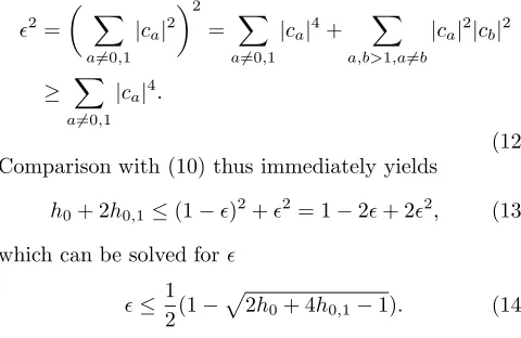
Fig. 2 shows how the bounds (16) for ǫ converge as confinement increases (γ→0) for the test Hamiltonian,
H4=
0 1 γ γ
1 1 0 0
γ 0 1.5 0
γ 0 0 1.7
. (20)
IV. FINITE SAMPLING FOURIER ANALYSIS
The previous section details how quantitative bounds on the subspace leakage can be obtained, in principle, from the Fourier spectrum of the Rabi data. However, to translate this method into a viable experimental protocol we need to consider the effects of finite sampling and taking the discrete Fourier transform (DFT), which raises several issues.
First the Nyquist criterion for sampling [31] must be satisfied, i.e., to avoid aliasing, some rough estimate of the Rabi periodTqubitis needed to guarantee that at least two sample points are chosen per oscillation period, i.e., ∆t≤Tqubit/2. The second issue that must be considered is the resolution of the Fourier spectrum. The frequency resolution ∆ωis given by ∆ω= 2π/tob, withtobthe total
FIG. 2: Upper and lower bounds onǫfor the four-level trial system governed by the Hamiltonian (20), characterized by a static coupling between the qubit states and a variable cou-plingγ to two higher levels. Asγ →0 the subspace leakage approaches 0 and the bounds forǫbecome more accurate.
within ∆ω of the primary peak then the DFT will com-bine the amplitudes for qubit and non-qubit transitions in the same frequency channel thus leading to an over-estimate of h0,1 and hence qubit confinement. To avoid such problems it is necessary to ensure that the total observation timetob is long enough such that non-qubit
transitions are distinguishable from the primary transi-tion. Thus, some estimates of the system parameters are required, although these do not need to be very accurate and will generally be known on theoretical or experimen-tal grounds.
Finally, the DFT has the property that a pure si-nusoidal signal will approach a delta function exactly if there is zero phase difference between the start and the end of the observed signal. If this phase match-ing condition is not met then all frequency peaks will broaden. Phase matching for system identification has al-ready been addressed for the identification of single qubit control Hamiltonians in [25] and we will follow the same approach, which essentially involves truncating the Rabi oscillation data at progressively greater values oftobsuch
as to maximize the trial function
P(tob) =
2F(ωp)−F(ωp−1)−F(ωp+ 1)
F(ωp−1) +F(ωp+ 1)
, (21)
whereF(ω) represents the amplitude of the Fourier Spec-trum at frequency ω andωp represents the frequency of
the maximum Fourier peak. The value oftobwhereP(tob)
is maximized represents the cut off time to the Rabi sig-nal that produced the best phase matching for the DFT. To simulate real experiments we numerically propa-gate the initial state |0i, under the Hamiltonian H, by
U(tk) = exp(−itkH) for discrete times tk =k∆t where
k= 0,1, . . . , KandK∆t=tob. A single measurement at
timetkis simulated by mapping the target stateU(tk)|0i
to {0,1}, where the probability of obtaining 0 is given byp0=|h0|U(tk)|0i|2; the ensemble average at a single
timetk is determined by dividing the number of zero
re-sults by the total number of repeat experimentsNe. For
the following numerical simulations we shall use the trial Hamiltonians
Ha =
0 1 0 0 0 1 1 0 0 0 0 0 1.5 0 0 0 0 0 1.7 0 0 0 0 0 2
, (22)
and
Hb =
0 1 0.01 0.005 0
1 1 0 0 0
0.01 0 1.5 0 0 0.005 0 0 1.7 0
0 0 0 0 2
, (23)
whereHa represents a five-level system with a perfectly
decoupled two-level subspace consisting of the two lowest energy states, whileHbrepresents a five-level system with
weak coupling between the qubit sub-manifold and two of the upper levels. The out-of-subspace coupling inHb
was chosen such that the leakage from the qubit subspace
ǫ≈7×10⁻⁴is small (too small to cause noticeable mod-ulations in the Rabi oscillations) yet significant (in fact above certain critical thresholds) for quantum computing applications. The part of the Hamiltonian governing the qubit dynamics was chosen arbitrarily and is common to all the Hamiltonians examined within this paper to maintain consistency between different simulations. The accuracy of the protocol is not affected by the choice of single qubit dynamics.
A. Estimating uncertainty in leakage bounds
Estimating uncertainties in the bounds forǫis crucial since for the majority of qubit systems it will be practi-cally impossible to prove that the evolution of the system under a given Hamiltonian is completely confined to the
SU(2) subspace, i.e., ǫ = 0. Instead, in practice it is sufficient for quality control purposes to experimentally confirm that the leakage from the qubit subspace is be-low a threshold value where it can effectively be ignored, i.e., it is the upper bound max(ǫ) that is relevant. The accuracy of our estimate for max(ǫ) will be primarily lim-ited by our ability to accurately determine the main peak heights h0 and h0,1 due to projection noise induced by the DFT.
Quantifying this uncertainty is relatively straightfor-ward. Defining the noise function ν(ω) of the Fourier spectrum to be the amplitudeν(ω) of each Fourier chan-nel excluding h0 = F(0) and h0,1 = F(ωp), the
of the noise function δh = sd[ν(ω)]. From this we can derive the uncertainty associated with max(ǫ)≡ǫu.
(δǫu)2=
∂ǫu
∂h0 2
(δh0)2+
∂ǫu
∂h01 2
(δh0,1)2
+ 2
∂ǫu
∂h0
∂ǫu
∂h01
δh0δh0,1= 3δh 2√2h0+ 4h1−1
.
(24)
δǫu can be reduced by increasing the number of
en-semble measurementsNetaken at each point in the Rabi
cycle. Figures 3 and 4 show how the estimate for ǫu
converges as Ne is increased for the Hamiltonians (22)
and (23), respectively. It should be noted that ǫu ≥0,
hence for each plot the lower error bars should only ex-tend to the zero point, but keeping the error bars sym-metrical around the data point makes the convergence behavior clearer. For large values of Ne, ǫu converges
to zero for the perfectly confined system governed by
Ha but the non-zero value ≈ 7×10⁻⁴ for the
imper-fectly confined system described by Hb. The respective
[image:6.612.329.552.54.224.2]observation times for each Hamiltonian were chosen to be tob = 30TRabi to ensure that all peaks are resolved, i.e., there are no contributions from additional transi-tions present within ∆ωof the primary peak.
FIG. 3: Convergence ofǫu as the number of ensemble
mea-surements, Ne, is increased for a system governed by the
Hamiltonian (23), characterized by perfect subspace confine-ment. The solid line represents the actual value ofǫm = 0.
Note error bars should only extend to zero asǫu≥0.
B. Numerical tests of error bound accuracy
To test the overall accuracy of the uncertainty esti-mates forǫu we can expect to obtain from realistic Rabi
oscillation data, we calculated the distance between the simulated value, ǫu, and the analytical value, ǫ′u,
calcu-lated directly from the Hamiltonian using Eq. 14.
[image:6.612.57.299.87.144.2]d(Hk) =|ǫu(Hk)−ǫ′u(Hk)|. (25)
FIG. 4: Convergence ofǫu as the number of ensemble
mea-surements,Ne, is increased for the imperfectly confined
sys-tem governed by the Hamiltonian (22). The solid line rep-resents the actual value ofǫu ≈ 7×10−
4
. Note error bars should only extend to zero asǫu≥0.
Where k ∈ [a, b] and δd(Hk) is the error in d resulting
from the error associated with estimating ǫu(Hk). We
first calculated the distanced(Hk) andδd(Hk) for 5000
simulated runs of two known trial Hamiltonians (Ha and
Hb) withǫ′u(Ha) = 0 andǫu′(Hb)≈7×10⁻⁴, respectively.
The distributions of d(Hk) for Ha and Hb (with Ne =
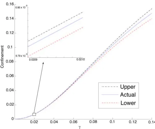
1024 andtobas in Figs 3 and 4 are shown in Figs 5 and 6, respectively. The average error 3δd(Hi),i∈[a, b], was
given by 3δd(Ha) ≈ 4.92×10⁻⁴, encompassing 99.9%
of the data, and 3δd(Hb) ≈5.02×10⁻⁴, encompassing
99.8% of the data, respectively.
FIG. 5: Distribution ofd(Ha) for 5000 separate simulations.
The average of the error, 3δd(Ha) is also shown, with
approx-imately 99.9% found within 3σofd= 0.
[image:6.612.65.288.349.519.2]FIG. 6: Distribution ofd(Hb) for 5000 separate simulations.
The average of the error, 3δd(Hb) is also shown, with
approx-imately 99.8% found within 3σofd= 0.
Hamiltonians of the form
HN =
9 X
k=0
Ek|kihk|+|0ih1|+
9 X
k=2
ak|0ihk|+ h.c. (26)
with {Ek} ≡ {0,1,1.5,2,2.4,2.5,2.9,3,3.3,4}. The
vec-tor~a = [a2, . . . , a9] was then chosen at random in two stages. First the dimensionality of~ais randomly selected, allowing the Hamiltonian to coherently drive any multi-level system, N ∈ [2,3, ..,10]. The non-zero coupling values were then randomly assigned such that each el-ement of~a was approximately two orders of magnitude less than the qubit coupling term to ensure that all of the multi-level systems had high confinement.
We randomly generated 5000 of these Hamiltonians and d(Hk) = |ǫu(Hk)−ǫ′u(Hk)| was calculated. The
average (analytical) value of ǫ′
u(Hk) for these 5000 trial
Hamiltonians was found to beǫ′
u(Hk) = 1.68×10⁻⁴. We
then examined the ratio,
R= Num{(d(Hk)−3δd(Hk)≤0)}
5000 , (27)
indicating the percentage of successful estimates of the subspace leakage within 3σ. This ratio was calculated to be R= 99.9%, with the confinement estimates being outside the error bounds for only three of the randomly generated Hamiltonians.
These results are consistent with the expectation that approximately 99.7% of the data should lie within 3σ
of the mean and demonstrates that our methodology for characterizing subspace leakage can indeed be expected to yield accurate upper bounds on the subspace leakage in the vast majority of cases.
V. EFFICIENCY OF THE PROTOCOL
The protocol presented in the previous section allows us to determine quantitative bounds on the subspace leakage for imperfect qubits by determining only the main peaks in the Fourier spectrum. An alternative strategy is to try to identify all peaks in the Fourier spec-trum. The presence of any peaks in addition to the two main peaks is indicative of subspace leakage and a quan-titative estimate of the leakage rate can be obtained by determining the heights of the additional peaks. Both approaches have potential advantages and disadvantages. The former approach requires only the identification of the two main peaks but these need to be clearly resolved and the peak heights determined with high precision. The latter approach does not require precise estimates of peak heights but relies on the detection of additional peaks, which for high confinement will be much smaller than the major peaks, and are likely to be difficult to dis-criminate from the noise floor. This raises the question which strategy is more efficient to decide if the subspace leakage for a given qubit is below a certain error thresh-old.
To answer this question, we performed a series of nu-merical simulations comparing the total number of mea-surements required to ascertain that the lower bound on the leakage rate ǫl = 1−
p
h0+ 2h0,1 > 0 within er-ror bounds, versus identifying a statistically significant third peak in the Fourier spectrum, indicating an out-of-subspace transition, for various trial Hamiltonians. For the purpose of the simulations we consider the following trial Hamiltonians
H3=
0 1 γ
1 1 0
γ 0 1.5
(28)
representing a system with a variable coupling γ to a third level, as well as the four-level system governed by the Hamiltonian (20) and a six-level system governed by
H6=
0 1 γ γ γ γ
1 1 0 0 0 0
γ 0 1.5 0 0 0
γ 0 0 1.7 0 0
γ 0 0 0 1.9 0
γ 0 0 0 0 2.2
, (29)
representing systems with variable but equal coupling to between one and four out-of-subspace levels, respectively. The lower bound, ǫl, is taken to be non-zero for a
discrete data set, if the analytical valueǫ′
l of the lower
bound calculated directly from the Hamiltonian exceeds six times the uncertainty,δ(ǫl), for the discrete data
cal-culated from the simulated Fourier spectrum, i.e.,
ǫ′l−6δ(ǫl)>0,
δ(ǫl) =
3δh
2p
h0+ 2h0,1
Six times the uncertainty in ǫl represents the total
dis-tance between the maximum and minimum possible value ofǫl(using a 3σupper and lower confidence bound) and
this interval should be smaller than the analytical value,
ǫ′
l.
A peakF(ω′) in the discrete Fourier spectrum is taken
to be significant if it is more than three standard devia-tionsδh= sd[ν(ω)] above the projection noise floor ¯ν(ω), i.e.,
F(ω′)−ν¯(ω)−3δh >0. (31)
[image:8.612.333.559.158.228.2]This definition will underestimate the number of ensem-ble measurements required slightly as it only represents the point where the third peak is greater than at least 99.7% of the noise channels.
FIG. 7: Number of ensemble measurements required to as-certain statistically significant subspace leakage (imperfect confinement) for the three-level system governed by (28) as a function of the (analytically calculated) confinement using the confinement equations (30) and by directly identifying the third transition peak.
For the simulations a range of out-of-subspace coupling strengths γ was chosen for each of the trial Hamiltoni-ans (28), (20) and (29), and the corresponding subspace leakage rate ǫ as well as the analytical lower bound ǫ′
l
computed. For each of the Hamiltonians we then simu-lated experimental Rabi data and computed the discrete Fourier spectrum. The observation time in all cases was 30 Rabi cycles and the number of ensemble measurements wasNe= 1024. The number of ensemble measurements
for the Rabi data simulations was gradually increased un-til a statistically significant third peak was found (31), or (30) was satisfied, respectively.
Fig. 7 shows the number of ensemble measurementsNe
necessary to conclude that the system is imperfect in the sense that leakage is statistically significant for the three-level system governed by (28) for both methods. The hor-izontal axis represents the analytical value of confinement
ǫ(γ). Both curves scale roughly 1/√Ne, which is
consis-tent with the scaling of the projection noise, and hence
the errors associated with estimatingǫl and detecting a
statistically significant third peak. For the three-level system it is clear that confirming imperfect confinement by verifying (30) requires more ensemble measurements than detecting a third peak according to (31). This is not too surprising since for a three-level system there is only one additional transition |0i ↔ |2i, and from the derivations of the confinement equations (9) we have,
1 = N−1
X
a=0
|ca|2
2
=
N−1
X
a=0
|ca|4+
X
a,b
|ca|2|cb|2 =h0+ X
a,b
ha,b,
(32)
i.e., there is a conservation law for the cumulative sum of all the peak heights. Hence, if the number of possible additional peaks is small, then for a given level of con-finement, the additional peaks will be greater, and thus easier to detect, than for a system with weak coupling to a large number of out-of-subspace levels, and hence many small transition peaks. We therefore conjecture that estimating subspace leakage using (30) will become preferable for a system with coupling to multiple out-of-subspace levels. The results of numerical simulations for the Hamiltonians (20) and (29), shown in Fig 8 support this conjecture. We observe the same general scaling be-havior as for the three-level system. For the four-level system it is clear that although searching for the addi-tional transition peak is still somewhat more efficient, the difference between both methods is small. For the six-level the curves have swapped position, i.e., using the confinement equations has become a more efficient way to ascertain statistically significant subspace leakage.
In Appendix A we have included simulations for sim-ilar Hamiltonians up to ten levels to show the effective crossover of the curves and how the efficiency difference between the two methods increases with the number of additional levels. Note that for all the simulations we have endeavored to look at approximately the same range of subspace leakage. From these simulations it is clear that searching for the third peak in the Fourier spec-trum is only really beneficial for systems with at most one extra transition. Hence, the proposed method for estimating subspace leakage will be more efficient than obvious alternatives in most cases.
VI. THE EFFECT OF DECOHERENCE
[image:8.612.65.286.249.416.2]FIG. 8: Number of ensemble measurements required to ascertain significant subspace leakage (imperfect confinement) for the four-level system governed by (20) [Fig. a] and the six-level system governed by (29) [Fig. b] using the confinement equations and identifying a third peak.
The study of arbitrary decoherence forN-level systems is a lengthy discussion, including Markovian and possi-ble non-Markovian processes. Even for the simpler case of Markovian decoherence we would need to consider the completeN-level decoherence model with all the associ-ated restrictions of completely positive maps [32]. Hence, we will instead only focus on a restricted case to show that, for a simple example, decoherence does not inval-idate the protocol. It should be stressed that this only represents a preliminary analysis under a specific model of decoherence. Further work will involve investigating more complicated and system-specific decoherence effects such as N-level dephasing and spontaneous emission as well as possible system specific non-Markovian decoher-ence. However, due to the extremely complicated nature of such an analysis we will limit our discussion to a spe-cific case.
We consider a perfectly confined qubit which under-goes Markovian decoherence and hence can be described by the quantum Liouville equation
∂tρ=−
i
~[H, ρ] + 3 X
k=1
ΓkLk[ρ] (33)
where,Lk[ρ] = ([Lk, ρL†k]+[Lkρ, L†k])/2,Hrepresents the
single qubit control Hamiltonian, and Lk are the
Lind-blad quantum jump operators, which describe the effect of the environment on the system, each parameterized by some rate Γk≥0.
For a basic decoherence analysis we restrict the Lind-blad operators to the Pauli set, {Lk} ={X, Y, Z}, and
consider a perfectly confined, control Hamiltonian of the form
H =d
2[cos(θ)Z+ sin(θ)X]. (34) This decoherence model is sufficient to describe pure de-phasing as well as symmetric population relaxation pro-cesses in any basis, although not asymmetric relaxation processes. Including each Pauli Lindblad term with an associated decoherence rate eliminates the problem of a preferential basis for qubit decoherence since any basis change of the overall system will only act to change the rates associated with each Lindblad operator.
We can solve the master equation under this model by using the Bloch vector formalism. Expressing the density matrix asρ(t) =I+x(t)X+y(t)Y+z(t)Z, Eq. (33) takes the form∂tS(t) =AS(t), whereS(t) = (x(t), y(t), z(t))T
and
A=
−2(Γy+ Γz) −dcos(θ) 0
dcos(θ) −2(Γx+ Γz) −dsin(θ)
0 dsin(θ) −2(Γx+ Γy)
.
(35) The Rabi oscillations under this evolution are described by the functionf(t) = Tr[P0ρ(t)] = (1/2)(1+z(t)), where
P0 = |0ih0|, with an initial state ρ(0) = |0ih0| =⇒
S(0) = (0,0,1)T. Taking the Fourier transform of f(t)
leads to the rather complicated general expression (B7) in Appendix B. The real component of this function describes three Lorentzians centered about ω = 0 and
Eq. (B7) aroundω= 0 andω =±dto obtain the func-tions [See Appendix B],
h0= cos2(θ) Γα
w2+ Γ2
α
,
h0,1= sin2(θ)
2
Γβ
(ω±d)2+ Γ2
β
,
(36)
where Γα = 2(Γy+ Γz+ cos2(θ)(Γx−Γz)) and Γβ =
Γx(1+sin2(θ))+Γy+Γz(2−sin2(θ)). In order to describe
how the maximum peak of each Lorentzian varies with Γ we integrateh0andh0,1around an intervalη of the peak height
h0(η) = cos2(θ) Z η
−η
Γα
ω2+ Γ2
α
=2 cos 2(θ)
π arctan
η
Γα
,
h0,1(η) =sin 2(θ) 2
Z ω+η
ω−η
Γβ
ω2+ Γ2
β
=sin 2(θ)
π arctan η Γβ . (37)
Hence, under decoherence the peak heights in the Fourier spectrum vary as a function of the integration window
η and the decoherence rates Γα,β. This is consistent
since as Γα,β → 0, both arctan functions approach π/2
and h0+ 2h0,1 = 1. The integration windowη is anal-ogous to frequency resolution of the Fourier transform ∆ω, while the total area of the Lorentzian is equal to the peak heights when Γx,y,z= 0. Hence for small Γx,y,z we
can simply choose the resolution of the Fourier transform such that the entire Lorentzian is essentially contained within the data channel of the primary peak.
Consider the case where we wish to ensure that the subspace leakage does not exceed ζ. Using the upper bound for the subspace leakage (14) we have, assuming that the integration interval is approximately equal to the frequency resolution of the DFT (i.e. η≈∆ω)
ζ= 1 2
1−
q
2h0(∆ω) + 4h0,1(∆ω)−1
,
(1−ζ)2+ 1
2 =
1 2+
cos2(θ)
π arctan ∆ω Γα +sin 2(θ)
π arctan
∆ω Γβ
π(1−2ζ)2
2 = arctan ∆ω
Γ
.
(38) Here the last line assumes that Γα ≈ Γβ = Γ. When
the Rabi frequency is much greater than the inverse of the decoherence rate (as necessary for any qubit realis-tically considered for quantum information processing), then the entire Lorentzian broadening caused by deco-herence will be contained within one frequency channel.
Thus, Eq. (38) allows us to calculate the maximum fre-quency resolution of the Fourier transform for successful leakage estimation using our protocol. For example, if Γ≈10−4t−1 and we wish to confirm that the subspace leakage is at most ǫmax = 10−8, then the resolution of the Fourier transform cannot exceed ∆f ≈250Hz if only the primary peak channels are used. Obviously, this re-striction on the frequency resolution can be lifted by in-cluding multiple channels around the central peak when estimating the peak area.
Although the decoherence model considered is not the most general possible case for an imperfectly confined control Hamiltonian, this calculation demonstrates that the effect of decoherence does not void the protocol for estimating subspace leakage for a common decoherence model. A more detailed analysis considering a full N -level decoherence model, including the effect of sponta-neous emission and absorption processes and the pos-sibility of system-specific non-Markovian decoherence is desirable but beyond the scope of the current paper.
VII. CONCLUSIONS
We have introduced an intrinsic protocol for “quantify-ing” the degree of subspace leakage for a realistic ‘qubit’ system. The protocol relies on very minimal theoretical assumptions regarding qubit structure and control, and utilizes a measurement model that is restrictive but ex-tremely common to a wide range of qubit systems. We have introduced a quantitative measure of subspace leak-age, and shown that the discretization noise as a result of finite sampling does not limit the ability of the protocol to quantify (with appropriate error/confidence bounds) the subspace leakage for well-confined (near perfect) qubits. The ability to experimentally characterize subspace leakage to a high degree of accuracy using system in-dependent methods that rely only on the intrinsic con-trol and measurement capacity of the quantum device, and can be automated, will be vital for the commercial success of quantum nano-technology. This protocol rep-resents one of the first steps in a general library of in-trinsic characterization techniques that will be required as “quality control” protocols once mass manufacturing of qubit systems becomes common.
Although, in this discussion, the qubit state|1iis only defined through the strongest transition it should be em-phasized that if confinement estimates are made on mul-tiple control fields (for example two separate Hamiltoni-ans which induce orthogonal axis rotations), the compu-tational|1istatemustbe common for both Hamiltonians. This is not a significant problem, since for well engineered qubits, the computational|1istate will be known on the-oretical grounds.
these schemes with other proposed methods for intrinsic characterization. Hopefully, in the near future, a com-plete set of characterization protocols will be developed which will augment large scale manufacturing techniques, allowing for efficient and speedy transition of quantum technology from the physics laboratory to the commer-cial sector.
APPENDIX A: EFFICIENCY COMPARISON FOR LEAKAGE DETECTION PROTOCOLS
The following simulations examined the minimal num-ber of ensemble measurements required to detect imper-fect qubits either via the confinement equations or by di-rectly detecting the third transition peak. Three-level, four-level and six-level Hamiltonians are found in the
main text, the additional simulations were performed for all other multi-level systems up to ten levels. The general form of each of the trial Hamiltonians are subsets of the ten-level system,
H10= 9 X
k=0
Ek|kihk|+γk(|0ihk|+|kih0|) (A1)
where{Ek} ≡ {0,1,1.5,1.7,1.9,2.2,2.5,2.7,3,3.2},γ1 = 1 andγk=γ fork6= 1.
For each lower level system the appropriate Hamilto-nian is simply formed by removing the appropriate num-ber of rows and columns fromH10(i.e. compareH4and
[image:11.612.68.536.267.464.2]H6 in Eqs. (20) and (29)). Each of these systems were simulated leading to the following results [Figs 9, 10 and 11],
FIG. 9: Number of ensemble measurements required to ascertain significant subspace leakage (imperfect confinement) for the five-level system [Fig. a] and the eight-level system [Fig. b] using the confinement equations and identifying a third peak.
APPENDIX B: SOLUTIONS TO THE DECOHERENCE MASTER EQUATION
Here we show the derivations of Eq. 36 by solving the Bloch equation∂tS(t) =AS(t), withAgiven in Eq. (35).
To solve this differential equation, we convert to Fourier space. Since the Fourier transform for a system governed by decoherence-induced semi-group dynamics is only de-fined fort≥0, we use the cosine and sine transforms
C[f(t);ω] = Z ∞
0
f(t) cos(ωt),
S[f(t);ω] = Z ∞
0
f(t) sin(ωt),
(B1)
noting that
C[f(t);ω]−iS[f(t);ω] = Z ∞
0
f(t)e−iωt=F+[f(t);ω]. (B2) Taking the sine and cosine transforms of∂tS(t) =AS(t),
noting that
C[ ˙f(t);ω] =ωS[f(t);ω]−f(0),
S[ ˙f(t);ω] =−ωS[f(t);ω], (B3)
gives
ωS[S(t);ω]−S(0) =AC[S(t);w],
FIG. 10: Number of ensemble measurements required to ascertain significant subspace leakage (imperfect confinement) for the seven-level system [Fig. a] and the nine-level system [Fig. b] using the confinement equations and identifying a third peak.
FIG. 11: Number of ensemble measurements required to as-certain significant subspace leakage (imperfect confinement) for the ten-level system using the confinement equations and identifying a third peak.
Combining these equations and setting S(ω) =
F+[S(t);ω] yields,
iωS(ω)−S(0) =AS(ω), (B5)
and hence
S(ω) =−(A−iωI)−1S(0). (B6)
The initial conditionS(0) = (0,0,1)T thus gives,
F T[z(t)] =− c
2d2+ (2Γ
x+ 2Γz+iω)(2Γy+ 2Γz+iω)
(c2d2+ (2Γ
x+ 2Γz+iω)(2Γy+ 2Γz+iω))(−2(Γx+ Γy)−iω)−d2s2(2Γy+ 2Γz+iω)
, (B7)
wherec= cos(θ) ands= sin(θ). The subsequent expan-sions are too lengthy to include here, however standard symbolic toolkits such as Mathematica can handle such expressions. The first step is to consider only the real component of F T[z(t)]. Next, the denominator is ex-panded to second order aroundω= 0 or ω=±d. After this, we expand the numerator and denominator, neglect-ing all terms of the form Γx,y,z/d and smaller, assuming
Γx,y,z ≪ d and being careful to note that for
expan-sions around ω = ±d we must keep terms of the form
ωΓx,y,z/d. After simplifying the expressions we find
h0= cos2(θ) Γα
w2+ Γ2
α
,
h0,1= sin2(θ)
2
Γβ
(ω±d)2+ Γ2
β
,
[image:12.612.65.288.298.466.2]where Γα = 2(Γy+ Γz+ cos2(θ)(Γx−Γz)) and Γβ =
Γx(1 + sin2(θ)) + Γy+ Γz(2−sin2(θ)). Confirming that
Eq. (36) describes three Lorentzian curves centered on
ω= 0 andω=±d.
ACKNOWLEDGMENTS
SJD acknowledges the support of the Rae & Edith Bennett Travelling Scholarship. SGS acknowledges
sup-port from an EPSRC Advanced Research Fellowship and the Cambridge-MIT Institute. DKLO acknowledges sup-port from Sidney Sussex College, Cambridge and SUPA. SGS and DKLO also acknowledge support from the EP-SRC QIP IRC (UK). SJD, JHC and LCLH are sup-ported in part by the Australian Research Council, the Australian Government and the US National Security Agency (NSA), Advanced Research and Development Activity (ARDA), and the Army Research Office (ARO) under contract number W911NF-04-1-0290.
[1] J. E. Mooij, T.P. Orlando, L. Levitov, L. Tian, C.H. van der Waal and S. Lloyd, Science.285, 1036-1039 (1999) [2] Y. Nakamura, C. D. Chen and J. S. Tsai, Nature
(Lon-don)398,786 (1999).
[3] M. R. Geller, E. J. Pritchett, A. T. Sornborger, F. K. Wilhelm. quant-ph/0603224 (2006).
[4] M.D. Lukin and P.R. Hemmer, Phys. Rev. Lett.842818 (2000).
[5] A.D. Greentree et. al., J. Phys: Condens, Matter 18 (2006) S825-S842
[6] J. Wrachtrup, S. Y. Kilin and A.P. Nizovtsev, Optics and Spectroscopy91429-437 (2001).
[7] J.I. Cirac and P. Zoller, Phys. Rev. Lett.74, 4091 (1995). [8] J. Clarkeet al., Science239, 992 (1988)
[9] A. Blais, A. M. van den Brink and A. M. Zagoskin. Phys. Rev. Lett.90, 127901 (2003).
[10] A.M. Steane, Phys. Rev. Lett.77, 793, (1996).
[11] R. Laflamme, C. Miquel, J. P. Paz, and W. H. Zurek, Phys. Rev. Lett.77, 198 (1996)
[12] D. Gottesman, Ph.D Thesis, quant-ph/9705052. [13] L.-A. Wu, M.S. Byrd and D.A. Lidar Phys. Rev. Lett.
89, 127901 (2002).
[14] M.S. Byrd, D. A. Lidar, L-A. Wu and P. Zanardi Phys. Rev. A.71, 052301 (2005).
[15] R. Fazio, G. Palma and J. Sieweret Phys. Rev. Lett.83, 5385 (1999).
[16] C. Mochor, Phys. Rev. A.69, 032306.
[17] J. Preskill, Introduction to Quantum Computation, pages 213269. World Scientific, Singapore, 1998. [18] M. Grassl, Th. Beth, T. Pellizzari Phys. Rev. A56, 33
(1997).
[19] J. Vala, K.B. Whaley and D.S. Weiss, Phys. Rev. A.72, 052318 (2005).
[20] K. Khodjasteh and D.A. Lidar Phys. Rev. A.68, 022322 (2003).
[21] P. Aliferis, B.M. Terhal Quant. Inf. Comp. 7, 139-156 (2006).
[22] J.H. Coleet al., Phys. Rev. A71, 062312 (2005). [23] J.H. Cole, S.J. Devitt and Lloyd. C.L. Hollenberg, J.
Phys. A: Math. Gen.39(2006), 14649-14658.
[24] S.J. Devitt, J.H. Cole, L.C.L. Hollenberg, Phys. Rev. A. 73, 052317 (2006).
[25] J.H. Coleet. al, Phys. Rev. A.73, 062333 (2006). [26] M. H. Devoret and R. J. Schoelkopf, Nature (London).
406, 1039 (2000).
[27] V. I. Conrad, A. D. Greentree, D. N. Jamieson and L. C.L. Hollenberg. Journal of Computational and Theoret-ical Nanoscience,2, 214 (2005).
[28] A. Aassime, G. Johansson, G. Wendin, R. J. Schoelkopf, and P. Delsing, Phys. Rev. Lett.86, 3376 (2001). [29] J. M. Martinis, S. Nam, J. Aumentado and C. Urbina,
Phys. Rev. Lett.89, 117901 (2002).
[30] G. Wendin and V. S. Shumeiko, cond-mat/0508729 (2005).
[31] R. N. Bracewell, The Fourier transform and its applica-tions, McGraw-Hill series in electrical and computer en-gineering. Circuits and systems. (McGraw Hill, Boston, 2000), 3rd ed.14. (Clarendon Press, Oxford, 1990). [32] S.G. Schirmer and A.I. Solomon, Phys. Rev. A. 70,