Simulation of associative learning with the replaced elements model

Running head: REPLACED ELEMENTS SIMULATION

Simulation of Associative Learning with the Replaced Elements Model

Steven Glautier

Abstract

Associative learning theories can be categorised according to whether they treat the representation of stimulus compounds in an elemental or configural manner. Since it is clear that a simple elemental approach to stimulus representation is inadequate there have been several attempts to produce more elaborate elemental models. One recent approach, the Replaced Elements Model (Wagner, 2003), reproduces many results that have until recently been uniquely predicted by Pearce’s Configural Theory (Pearce, 1994). Although it is possible to simulate the Replaced Elements Model using “standard”

Simulation of Associative Learning with the Replaced Elements Model

A simple application of the Rescorla-Wagner Model (RWM) of associative learning treats stimulus inputs as simple experimenter-defined elements (Rescorla & Wagner, 1972). For example, in Mackintosh’s 1976 study of overshadowing in rats, a compound of two stimuli, A and B, was trained as a signal for electric shock

(Mackintosh, 1976). In this procedure, according the RWM, the associative strength of A and B would increase on each trial as specified in Equation 1.

∆

V

=

α

β

(

λ

-

(

VA

+

VB

)

)

Equation 1

Equation 1 states that the change in associative strength for each of A and B (∆Vn) is a function of two learning rate parameters (α and $) and the difference between an asymptote (λ) and the sum of the strengths of A and B on the previous trial (VAn-1 and VBn-1). In this model, after a number of trials, it would be expected that VA and VB would both approach 1/2λ is A and B are of equal salience. In contrast, if A was trained alone its asymptotic associative strength would be λ. Unfortunately this does not lead to the prediction that the response to A after training with an AB compound will be half of the magnitude of that seen to A after training with A alone. This prediction does not follow for at least two reasons. First, there is no accepted mapping between associative strength and response strength and second, there is no accepted account of the process by which associative mechanisms treat stimulus compounds.

The assumption that stimulus compounds are treated by the associative

mechanism simply as experimenter-defined elements has been challenged on a number of grounds. For example, there are numerous experiments that show both animals and humans can learn to respond more to the elements than to the compound in negative patterning discriminations (e.g. Woodbury, 1943; Lachnit & Kimmel, 2000). In negative patterning, elements are reinforced whereas a compound of those elements is

a unique configural cue (Wagner & Rescorla, 1972) the RWM can solve this type of problem. For instance, the experimenter may present a light (A) and a tone (B) but the organism represents the light-tone compound as ABX, where X is the unique configural cue that occurs in the presence of the AB compound. Apart from the fact that negative patterning discriminations can be learned some experimental evidence has been provided that a unique-cue is actually generated when two stimuli are compounded (e.g. Rescorla, 1973).

Negative patterning discriminations have been dealt with in alternatives to the unique-cue extension of the RWM. In one approach, a configural theory (CT), has been proposed (Pearce, 1987; Pearce, 1994). In Pearce’s CT changes in associative strength are calculated in a similar way to the computations in the RWM. But, CT assumes that entire stimulus patterns gain associative strength. Thus, in negative patterning, three distinct patterns would undergo associative changes; a representation of A, a

representation of B, and a representation of AB. Because the AB compound has its own distinct representation and associative strength the model is readily able to predict that negative patterning discriminations can be learned. Furthermore, CT, has the advantage over the unique-cue version of the RWM because the unique-cue RWM predicts

summation effects, despite the fact that summation does not always occur. For example Aydin and Pearce have reported that responding to an AB compound did not exceed responding to the previously reinforced A and B elements (Aydin & Pearce, 1995; Aydin & Pearce, 1997). The RWM would predict that after training A and B the associative strengths of A and B would summate in an AB compound and hence the response to AB should exceed that seen to either A or B alone.

parameter, R, varies. As a result the model is a challenge both to alternative elemental (e.g. RWM and it’s unique-cue variants) and configural accounts (Pearce, 1987; Pearce, 1994) of associative learning which incorporate different mechanisms for processing of stimulus compounds. The current paper outlines the key features of the REM and describes a method for specifying the REM elements so that REM predictions can be generated computationally. In addition, examples simulations are presented. These show differential predictions of the REM and Pearce’s Configural Theory.

In essence, the REM extends the idea that unique configural cues can be produced whenever two or more stimuli are compounded. The suggestion is that representation of a stimulus is comprised of three types of element: (a) elements that represent the stimulus independently of the context set by other stimuli, (b) elements that represent the stimulus in a context that encodes the presence of other stimuli, and (c) elements that represent the stimulus in a context that encodes the absence of other stimuli. For example, in order to represent a stimulus world consisting of two stimulus components A and B the REM specifies elements of A that are always active when A occurs (Ai, read “A independent” elements), elements of A that represent A in the presence of B (AB, read “A in the presence of B” elements), and elements of A that represent A in absence of B (Ab, read “A in the absence of B” elements). Representation of B is similarly specified by Bi, BA, and Ba elements. The parameter R (0 ≤ R ≤ 1), dictates the proportion of stimulus elements that encode the context set by the presence and absence of other stimuli and variation in R renders the REM capable of behaving either elementally or configurally. For instance, when R = 0 the entire representation of A is made up of Ai elements – there is no encoding of the presence or absence of other stimuli. When R = 0.5 half of the representation of A is made up of Ai elements and other half encodes the

presence/absence of other stimuli. This scheme will be expanded upon in the description of the simulation program below (for further details see Wagner, 2003).

code Ab, and one to code AB and the B component would be represented likewise, one for element Bi, one for Ba, and one to code BA. The proportional representations

required for A, B, and AB trials with R=0.5 are illustrated in the left-hand-side of Table 1 which shows how the conditioned stimulus (CS) inputs to a conventional RWM

simulation of this scenario could be presented in a binary vector with length 6. Referring to Table 1, conditioning on a trial involving CS A alone would require re-calculation of Ai and Ab elements whilst a trial with an AB compound would require computations on Ai, AB, Bi, and BA elements.

Simulations of this two-component world are also possible for other values of R. The right-hand-side of Table 1 shows proportional representations required for an R-value of 0.25. These proportions can be represented using a binary vector of length 10 for the CS encoding, three elements for each of Ai and Bi and one element for each of Ab, AB, Ba, and BA. On a trial with CS A alone all three Ai elements would need their associative strengths adjusted, along with the single Ab element. Once the correct proportional representations of different elements for each conditioning trial are

established the simulation can then proceed keeping track of the associative strengths of elements in the conventional way. Equation 1 shows how this works on conditioning trials involving A alone.

∆ V ₌ α β λ -

Σ

k = 1

3 VAi ⎛ ⎜ ⎜ ⎝ ⎞ ⎟ ⎟ ⎠ + VAb ⎛ ⎜ ⎜ ⎝ ⎞ ⎟ ⎟ ⎠ ⎛ ⎜ ⎜ ⎜ ⎝ ⎞ ⎟ ⎟ ⎟ ⎠ Equation 2

Table 2 gives the results of a RWM simulation of REM for a sequence of three reinforced trials involving A, AB, and then B with R=0.25 based on Equation 2 with

αβ=0.125. For more complex simulations involving multiple stimuli e.g. a three stimulus world of A, B, and C or four stimuli, A-D and arbitrary R-values the total number of stimulus elements required to represent the required proportions becomes very large and construction of the vectors for different stimulus patterns is complex. As a result a more effective method is suggested below.

Method

The alternative approach involves using single elements to represent each REM element and weighting the updates on the associative strengths of those elements to reflect their proportional representations in REM. Equation 3 illustrates the use of these weights in simulation of trials involving A alone.

∆

V

=

ω

α

β

(

λ

-

(

VAi

+

VAb

)

)

Equation 3

Enumeration of REM components

Given a list of the stimuli that are present on a trial, and a list of stimuli that are absent, the algorithm REMElements (StimuliPresent, StimuliAbsent) returns the list of REM elements that are assumed to be active and whose associative strengths will need updating on that trial (see Appendix 1 and text below for details of this algorithm). Returning to the two component world involving A and B, the REM element list for a trial involving A alone would be returned from a function call of the form

REMElements(A, b). The first parameter of this function call takes a list of the

components that are actually present (in upper case) and the second parameter takes a list of elements that are absent (in lower case). If a three component world (components A-C) was simulated then a list of REM elements for a trial involving BC would be generated by the call REMElements (BC, a). The outputs from this algorithm for different stimulus combinations for a three component simulation are given in Table 4. The left-hand-side of Table 4 lists all of the REM elements that could be active in the three component world. The main body of the table contains 0s and 1s to indicate whether an REM element is active given the presence of the stimulus components listed across the top of the table. For example, if AB was presented then REM elements Ai, AB, Ac, ABc, Bi, BA, Bc, BAc would be activated and the call REMElements (AB, c) would generate the list of strings A, AB, Ac, ABc, B, BA, Bc, BAc corresponding to those elements. Note that A, B, and C correspond to Ai, Bi, and Ci – the suffix i, used in the text, is dropped as redundant.

Appendix 1 gives further details of the algorithm that generates a list of all the REM elements present on a trial for an arbitrary number of components. This algorithm can be incorporated into a simulation program using two lists TList and SList. A new TList is created on each trial of the simulation and uses the REMElements function to establish which elements are present on that trial. SList is created once for each

set to a default (e.g. 0). Next, the change in associative strength for each element of TList is computed using Equation 4 and these change values are added to the associative strengths already recorded for each element in TList.

=

∆

V

k

ω

α β

⎛

⎝

⎜⎜

⎜

⎞

⎠

⎟⎟

⎟

−

λ

⎛

⎝

⎜⎜

⎜

⎞

⎠

⎟⎟

⎟

∑

V

In Equation 4 the summation in the error term (the major parenthesised term) is over the n elements present in TList, i.e. this is the sum of the associative strengths of all of the elements used in REM to represent the particular pattern of CSs present on that trial. The

ω values for each element are required (see below) but once these changes have been calculated these values are added to those already present in TList and to complete the trial SList is updated with new associative strengths for all of those stimuli that are in TList.

Calculation of REM component weights

example, AB. Thus, different ω values are required for REM components as the

dimensionality of the simulation varies. The method for determining the ω values ensures that the results of a simulation will be the same whatever the dimensionality of the

simulation e.g. a sequence of A+, AB+, B+ would yield the same results whether

conducted in a 2 stimulus or a 4 stimulus simulation. Calculation of the required weights can be achieved using the binomial expansion in Equation 5.

R

+

S

(

)

Equation 5

Equation 5 is a general expression for REM weights where D is the

dimensionality of the simulation being conducted and S = 1-R. In a simulation of a two stimulus world the elements Ab, AB, Ba, and BA have a weight of R whereas Ai and Bi have a weight of (1-R). In simulation of a three stimulus world Equation 5 expands to

R2 + 2 RS + S2

Equation 6

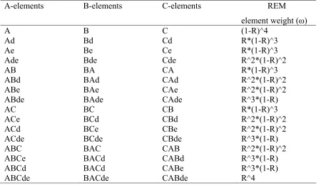
and the weights R^2, R(1-R), and (1-R)^2 are applied to REM element strings (generated as described in Appendix 1) with lengths 3, 2 and 1, respectively. See Tables 1, 4, and 6 for examples of weights generated for elements from 2, 3, and 5-D simulations. Table 7 lists all weights needed for models involving up to 6-D simulations.

Discussion and Example Simulations

Although simulations of REM can be carried out using conventional RWM approaches, generation of the required elements is cumbersome, but the foregoing illustrates an alternative method for simulation of the REM. The method includes

RWM. For example, the RWM cannot generate appropriate predictions for non-linear discriminations such as negative patterning. Whilst it is possible for the RWM to solve this type of discrimination using unique cues to code stimulus compounds the unique-cue approach still predicts summation when summation effects do not always occur (Aydin et al., 1995; Aydin et al., 1997).

Both Pearce’s configural model (Pearce, 1994) and the REM are alternatives to the RWM that can generate the correct predictions for the negative patterning design and both indicate that summation may or may not occur. In the case of Pearce’s model summation is predicted when there are common elements to the trained stimuli. For example a test on ABC will lead to summation after reinforced AC and BC trials. In the case of the REM summation is predicted to occur with low R values. What then

differentiates these models? Wagner referred to several experiments in which the

different predictions of the RWM and Pearce’s configural model had both been supported and showed how the REM could predict the outcomes subject to variation in R (Wagner, 2003). Nonetheless, the most interesting tests of these theoretical models are from designs that make parameter free differential predictions.

patterning discrimination (Figure 2). According to the predictions of CT there is equivalence in the similarity relations in the two discriminations so the simple and complex design should be equally difficult. In the REM though, the complex

discrimination is predicted to be easier because more stimuli are present on each trial and so both excitatory and inhibitory conditioning proceed more rapidly. When R=1 there is no overlap between the non-reinforced stimulus compounds so the elements representing AB (simple) and ABCD (complex) do not become inhibitory and the discrimination only involves increases in excitatory strength for the reinforced stimuli A/B (simple) and AB/CD (complex). Although increasing the complexity of a negative patterning design has been found to increase the difficulty of the discrimination, in support of CT, this result has been found by increasing the similarity between the reinforced and non-reinforced cues (Pearce et al., 1993).

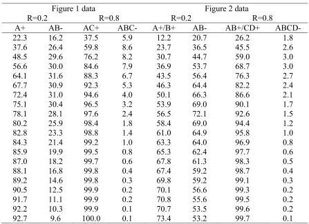
The simulations shown in Figures 1 and 2 were carried out as follows. The learning rate parameter α was set at 0.005, while $ was set at 1 or 0.5 for reinforced and non-reinforced trials respectively. For the simulations in Figure 1, 1800 trials of each type were carried out in a randomized order. The simulation was stopped after every 45 trials and tests carried out. The values in the figure are averaged over 10 runs. The

Author Note

Steven Glautier, School of Psychology, Southampton University, UK.

I would like to thank Alan Wagner for his helpful comments and elaborations on early attempts at simulation and Ed Redhead for discussion and comments on a draft of this paper.

Reference List

Aydin, A. & Pearce, J. M. (1995). Summation in autoshaping with short and long duration stimuli. Quarterly Journal of Experimental Psychology, 42B, 215-234.

Aydin, A. & Pearce, J. M. (1997). Some determinants of response summation. Animal Learning and Behavior, 25, 108-121.

Brandon, S., Vogel, E. H., & Wagner, A. R. (2000). A componential view of configural cues in generalization and discrimination in Pavlovian conditioning. Behavioural and Brain Research, 110, 67-72.

Lachnit, H. & Kimmel, H. D. (2000). Experimental manipulation of a unique cue in Pavlovian SCR conditioning with humans. Biological Psychology, 53, 105-129.

Mackintosh, N. J. (1976). Overshadowing and stimulus intensity. Animal Learning & Behavior, 4, 186-192.

Pearce, J. M. (1994). Similarity and discrimination: A selective review and a connectionist model. Psychological Review, 101, 587-607.

Pearce, J. M. (1987). A model of stimulus generalisation for Pavlovian conditioning. Psychological Review, 94, 61-73.

Rescorla, R. A. (1973). Evidence for a "unique stimulus" account of configural conditioning. Journal of Comparative and Physiological Psychology, 85, 331-338.

Rescorla, R. A. & Wagner, A. R. (1972). A theory of Pavlovian conditioning: variations in the effectiveness of reinforcement and non-reinforcement. In A.H.Black & W. F. Prokasy (Eds.), Classical Conditioning II: Current Research and Theory (pp. 64-69). New York: Appleton Century Crofts.

Sutton, R. S. & Barto, A. G. (1981). Toward a modern theory of adaptive networks: expectation and prediction. Psychological Review, 88, 135-170.

Wagner, A. R. (2003). Context-sensitive elemental theory. Quarterly Journal of Experimental Psychology, 56B, 7-29.

Wagner, A. R. & Brandon, S. E. (2001). A componential theory of Pavlovian conditioning. In R.R.Mowrer & S. B. Klein (Eds.), Handbook of Contemporary Learning Theories (pp. 23-64). Mahwah, N.J.: Lawrence Erlbaum Associates.

Wagner, A. R. & Rescorla, R. A. (1972). Inhibition in Pavlovian conditioning: Application of a theory. In R.A.Boakes & M. S. Halliday (Eds.), Inhibition and Learning (pp. 301-340). London: Academic Press Inc.

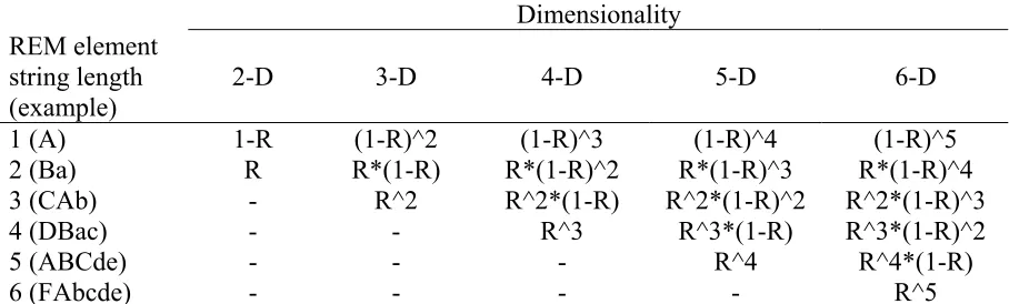
CSs

R=0.5 R=0.25

Input elements

A B AB A B AB REM element

weight (ω)

Ai 1 0 1 3 0 3 1-R

Ab 1 0 0 1 0 0 R

AB 0 0 1 0 0 1 R

Bi 0 1 1 0 3 3 1-R

Ba 0 1 0 0 1 0 R

BA 0 0 1 0 0 1 R

Table 1. An illustration of the vector inputs required for a RWM based simulation of REM for R-values of 0.5 and 0.25 to represent all combinations of two component

stimuli, A and B. With R=0.25 three elements are required to represent each of Ai and Bi. The far right-hand column shows REM weights for each element.

Trial λ-ΣV Ai1 Ai2 Ai3 Ab AB Bi1 Bi2 Bi3 Ba BA A+ 1.0000 0.1250 0.1250 0.1250 0.1250 0.0000 0.0000 0.0000 0.0000 0.0000 0.0000 AB+ 0.6250 0.2031 0.2031 0.2031 0.1250 0.0781 0.0781 0.0781 0.0781 0.0000 0.0781 B+ 0.7656 0.2031 0.2031 0.2031 0.1250 0.0781 0.1738 0.1738 0.1738 0.0957 0.0781

Trial λ-ΣV Ai Ab AB Bi Ba BA A+ _{1.0000 0.3750 0.1250 0.0000 0.0000 0.0000 0.0000} AB+

0.6250 0.6094 0.1250 0.0781 0.2344 0.0000 0.0781 B+

0.7656 0.6094 0.1250 0.0781 0.5215 0.0957 0.0781

Stimulus components REM

element string A B C AB AC BC ABC element weight (REM ω)

Ai 1 0 0 1 1 0 1 (1-R)^2

AB 0 0 0 1 0 0 1 R*(1-R)

Ab 1 0 0 0 1 0 0 R*(1-R)

AC 0 0 0 0 1 0 1 R*(1-R)

Ac 1 0 0 1 0 0 0 R*(1-R)

ABC 0 0 0 0 0 0 1 R^2

ABc 0 0 0 1 0 0 0 R^2

ACb 0 0 0 0 1 0 0 R^2

Abc 1 0 0 0 0 0 0 R^2

Bi 0 1 0 1 0 1 1 (1-R)^2

BA 0 0 0 1 0 0 1 R*(1-R)

Ba 0 1 0 0 0 1 0 R*(1-R)

BC 0 0 0 0 0 1 1 R*(1-R)

Bc 0 1 0 1 0 0 0 R*(1-R)

BAC 0 0 0 0 0 0 1 R^2

BAc 0 0 0 1 0 0 0 R^2

BCa 0 0 0 0 0 1 0 R^2

Bac 0 1 0 0 0 0 0 R^2

Ci 0 0 1 0 1 1 1 (1-R)^2

CA 0 0 0 0 1 0 1 R*(1-R)

Ca 0 0 1 0 0 1 0 R*(1-R)

CB 0 0 0 0 0 1 1 R*(1-R)

Cb 0 0 1 0 1 0 0 R*(1-R)

CAB 0 0 0 0 0 0 1 R^2

CAb 0 0 0 0 1 0 0 R^2

CBa 0 0 0 0 0 1 0 R^2

Cab 0 0 0 0 0 0 0 R^2

Σ weights 1 1 1 2 2 2 3

Table 4. Illustration of REM element strings required to represent all combinations of CSs in a three-component world involving A, B, and C. The weights (ω) required in Equation 3 for each element are shown in the right-hand column and the sum of the weights for each trial is given in the bottom row. Note, for the purpose of weight

A B C

B C A

C A B

Table 5. Stimulus present strings after rotations in the function REMElements. The shading indicates the tails used in the calls on Combinations used in the function GeneratePresentStimuliList, see Appendix 1.

A-elements B-elements C-elements REM

element weight (ω)

A B C (1-R)^4 Ad Bd Cd R*(1-R)^3 Ae Be Ce R*(1-R)^3 Ade Bde Cde R^2*(1-R)^2 AB BA CA R*(1-R)^3 ABd BAd CAd R^2*(1-R)^2 ABe BAe CAe R^2*(1-R)^2 ABde BAde CAde R^3*(1-R) AC BC CB R*(1-R)^3 ACe BCd CBd R^2*(1-R)^2 ACd BCe CBe R^2*(1-R)^2 ACde BCde CBde R^3*(1-R) ABC BAC CAB R^2*(1-R)^2 ABCe BACd CABd R^3*(1-R) ABCd BACd CABe R^3*(1-R) ABCde BACde CABde R^4

Dimensionality REM element

string length (example)

2-D 3-D 4-D 5-D 6-D

1 (A) 1-R (1-R)^2 (1-R)^3 (1-R)^4 (1-R)^5

2 (Ba) R R*(1-R) R*(1-R)^2 R*(1-R)^3 R*(1-R)^4 3 (CAb) - R^2 R^2*(1-R) R^2*(1-R)^2 R^2*(1-R)^3

4 (DBac) - - R^3 R^3*(1-R) R^3*(1-R)^2

5 (ABCde) - - - R^4 R^4*(1-R)

6 (FAbcde) - - - - R^5

Figure captions

Figure 1. Simulations of feature negative discriminations with (AC+, ABC-) and without (A+, AB-) common features. The predictions from Pearce’s configural model and from the REM with R=0.2 and R=0.8 are shown. The abscissa shows associative strength (V) x 100. See text for further details.

CR

0

20

40

60

80

100

A+

AB-

AC+

ABC-

CR

0

20

40

60

80

100

Trial block

CR

0

20

40

60

80

100

Configural model

REM R = 0.2

CR

0

20

40

60

80

100

CR

0

20

40

60

80

100

CR

0

20

40

60

80

100

A+/B+

AB-AB+/CD+

ABCD-Configural model

REM R = 0.2

REM R = 0.8

Appendix 1

The function REMElements (StimuliPresent, StimuliAbsent) takes two strings as its parameters, StimuliPresent and StimuliAbsent, and returns a list of strings. Each string on the returned list represents one of the REM elements that are present, given the

parameters, and the returned list is a complete enumeration of those elements required by the REM to represent the CSs present on that trial. The StimuliPresent string is an

enumeration of the CSs actually present, the StimuliAbsent string enumerates those CSs that are absent. For example in simulation involving four CS components (A-D), a trial with A alone would require a call REMElements(A,bcd) whereas a trial of ACD would need the call REMElements (ACD, b). In a simulation involving five CS components (A-E) the same trials would be called with REMElements (A,bcde) and REMElements (ACD,be).

REMElements makes use of three lists. AList is generated from the StimuliAbsent string whereas PList is generated from the StimuliPresent string. RList is the list that the function returns, it is generated by merging AList and PList. In pseudocode the principle algorithm of REMElements is:

AList:=GenerateAbsentStimuliList(StimuliAbsent); PList:=GeneratePresentStimuliList(StimuliPresent); RList:=Merge(AList,PList);

GenerateAbsentStimuliList operates by generating substrings, of length 1..n, each of which is a unique combination of characters from the string StimuliAbsent, where n is the length of StimuliAbsent. In pseudocode:

i:=0;

while (i< length(StimuliAbsent))

ReturnList:=ReturnList+Combinations(i+1, StimuliAbsent); i:=i+1;

The call Combinations(i+1, StimuliAbsent) returns a list of all combinations of characters in StimuliAbsent with length i+1. As examples, the call Combinations(1, abc) would return a list containing elements a,b, and c; Combinations(2, abc) would return elements ab, ac, and bc; whereas Combinations(3, abc) would return a list with a single element abc. As a result the call GenerateAbsentStimuliList(abc) would produce the ReturnList consisting of elements a, b, c, ab, ac, bc, abc. The call GenerateAbsentStimuliList(de) would produce the ReturnList consisting of elements d, e, de.

GeneratePresentStimuliList operates on similar principles but produces calls on the Combinations function with substrings of StimuliPresent. Substrings of

StimuliPresent are generated by rotating the characters of StimuliPresent and, after each rotation, calling Combinations on the tail of StimuliPresent. Table 5 shows the first two rotations of StimuliPresent that would occur in a call of

GeneratePresentStimuliList(ABC). The number of rotations in each call of

GeneratePresentStimuliList is equal to the length of the StimuliPresent string and the last rotation returns StimuliPresent to its original state. The pseudocode runs:

i:=0; j:=0;

while (i< length(StimuliPresent))

ReturnList:=ReturnList+Head(StimuliPresent); while(j<length(StimuliPresent)-1)

TempList:=Combinations(j+1, Tail(StimuliPresent));

ReturnList:=ReturnList+Prepend(TempList,Head(StimuliPresent)); j:=j+1;

end while;

Rotate(StimuliPresent); i:=i+1;

end while;

characters of its parameter to the left and the “overflow” character is appended to the end, as indicated in Table 5. Prepend is a function that takes a list of strings as a target and for every string in that list it prepends a character before returning the list with the prepends. The result of the call GeneratePresentStimuliList(ABC) returns a list consisting of the elements A, AB,AC, ABC; B, BC, BA, BCA; C, CA, CB, CAB. The elements listed after semi-colons occur after rotations of StimuliPresent.

The final function of REMElements is Merge(AList,PList). It works by creating a list of strings that contains each element of PList plus each element of PList combined with each element of AList as follows:

i:=0; j:=0;

while (i<length(PList))

ReturnList:=ReturnList+PList[i]; while (j<length(AList))

ReturnList:=ReturnList+(PList[i]+AList[j])); j:=j+1;

end while; i:=i+1;

end while;

Using the examples above, if PList consisted of elements A, AB,AC, ABC; B, BC, BA, BCA; C, CA, CB, CAB and AList consisted of elements d, e, de, as they would after GenerateAbsentStimuliList(de) and GeneratePresentStimuliList(ABC) then Merge(AList, PList) would result in the list shown in Table 6. Thus, in a simulation of a

Appendix 2

Figure 1 data Figure 2 data

R=0.2 R=0.8 R=0.2 R=0.8

A+ AB- AC+ ABC- A+/B+ AB- AB+/CD+ ABCD-