University of Southampton Research Repository
ePrints Soton
Copyright © and Moral Rights for this thesis are retained by the author and/or other copyright owners. A copy can be downloaded for personal non-commercial
research or study, without prior permission or charge. This thesis cannot be
reproduced or quoted extensively from without first obtaining permission in writing from the copyright holder/s. The content must not be changed in any way or sold commercially in any format or medium without the formal permission of the
copyright holders.
When referring to this work, full bibliographic details including the author, title, awarding institution and date of the thesis must be given e.g.
UNIVERSITY OF SOUTHAMPTON
Faculty of Engineering, Science and Mathematics School of Geography
Exploring Equifinality in a Landscape Evolution Model
by
Nicholas Alan Odoni
Thesis submitted for the degree of Doctor of Philosophy (Ph.D.)
UNIVERSITY OF SOUTHAMPTON
ABSTRACT
FACULTY OF ENGINEERING, SCIENCE AND MATHEMATICS SCHOOL OF GEOGRAPHY
Doctor of Philosophy
EXPLORING EQUIFINALITY IN A LANDSCAPE EVOLUTION MODEL by Nicholas Alan Odoni
Model equifinality is the property by which very similar model outputs can be generated by many different combinations of model inputs. It is known in numerical models used in other disciplines, and is thought to be likely in landscape evolution models (“LEMs”) also, as they incorporate many process parameters of uncertain value. LEM equifinality, if pervasive, would be a serious obstacle to falsifying working hypotheses and would frustrate landscape evolution research, but to date it has not been quantified. This is attempted here, by
sampling a LEM’s response in its parameter space. A well known LEM (‘GOLEM’, Tucker & Slingerland, 1994), used here as an exemplar, is applied to evolution of a c. 38 km2, 4th order catchment in the Oregon Coast Range. Ten of GOLEM’s parameters are selected for variation, covering mass movement, channel formation, fluvial erosion and weathering processes, and value ranges appropriate for the catchment are established from published data and calibration. Parameter space sampling is then carried out using a response surface methodology approach which reduces by c. 3 orders of magnitude the simulation run size needed to explore the 10-D parameter space. Initial simulations are run sampling the space according to a central composite design of 149 targeted parameter value combinations, which afford estimation of all parameter main and two-way interaction effects. Model outputs at 100,000 years are summarised by four metrics (sediment yield, drainage density, sediment delivery ratio, and a topographic metric), which serve as landscape descriptors. Equations, or “metamodels”, are derived by regression to describe each metric as a function of the GOLEM parameters, and further simulations allow testing and improvement of model fits (R2 of c. 98% for the sediment yield, drainage density and sediment delivery ratio, and c.
CONTENTS
PAGE
Abstract ...i
Contents ...ii – vi List of figures ...vii – ix List of tables ...x
Author’s declaration ...xi
Dedication ...xii
Acknowledgments ...xiii
CHAPTER 1: INTRODUCTION AND RESEARCH AIMS ... 1
1.1 General theme ... 1
1.2 Equifinality and model equifinality ... 3
1.2.1 Equifinality as a concept ... 3
1.2.2 Uncertainty and the possibility of equifinality in LEMs... 8
1.3 Variables used in LEMs and their influence on output...17
1.3.1 Table of example LEM studies ... 17
1.3.2 Research themes, and association of variables with model output ...21
1.3.3 Summary of introductory review ... 23
1.4 Formulation of the research aims, and thesis structure... 24
CHAPTER 2: LANDSCAPE EVOLUTION MODEL PARAMETERS AND PARAMETER SPACES... 27
2.1 Introduction ... 27
2.2 General characteristics of LEMs... 28
2.2.1 Table of reviewed models ... 28
2.2.2 Spatial domain, time steps and state variables ... 32
2.2.3 Driving conditions – climate, base level and uplift...33
2.3 Process parameters and mass continuity...34
2.4 Weathering ... 37
2.4.1 Basic processes and form of mathematical relationship ... 37
2.4.2 Weathering process equations and adjustable parameters ...38
2.5 Mass movement ... 40
2.5.1 Movement mechanisms, material type and dispersal...40
2.5.3 Nearest neighbour representations of slow mass movement ... 44
2.5.4 Nearest neighbour representations of combined speed and fast mass movements ... 45
2.5.5 Extended dispersal representations of mass movement ... 48
2.6 Fluvial erosion and sediment transport ... 49
2.6.1 Driving conditions and general implementation ... 49
2.6.2 Basic types of equation ... 51
2.6.3 Fluvial transport equations used in LEMs ... 55
2.6.4 Channels and channelled transport in LEMs ... 61
2.6.5 Section summary – fluvial transport, erosion, and related functions ... 66
2.7 Typical parameter spaces of LEMs... 67
2.7.1 Typical parameter requirements in LEMs...68
2.7.2 Table of parameter values appropriate in modelling studies ... 71
CHAPTER 3: METHODOLOGY – GENERAL APPROACH TO QUANTIFICATION AND PARAMETER SAMPLING ...76
3.1 Introduction ... 76
3.2 Parameter space sampling issues, and choice of methodology and its conceptual basis 77 3.2.1 Parameter spaces, simulations and experiment run sizes... 77
3.2.2 The ‘metamodel’ concept...79
3.3 Sampling and experiment designs ... 82
3.3.1 Basic concepts ... 82
3.3.2 Monte Carlo and Latin Hypercube sampling schemes ... 86
3.3.3 Factorial, fractional factorial and central composite designs... 88
3.3.4 Choice of sampling method ... 94
3.4 Choice of LEM and model description...97
3.4.1 Choice of model ... 97
3.4.2 Description of GOLEM... 97
3.5 Implementation in GOLEM ... 104
3.5.1 Study catchment ... 104
3.5.2 Parameterisation of GOLEM for the Smith River simulations ... 110
CHAPTER 4: MODEL OUTPUT, CHOICE OF METRICS AND DERIVATION OF THE
METAMODELS ... 115
4.1 Introduction ... 115
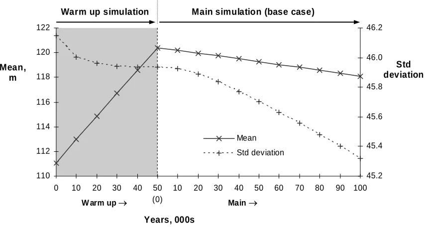
4.2 Output from the warm up and base case simulations ... 116
4.2.1 Evolution of topography ... 116
4.2.2 Evolution of the drainage network ... 119
4.2.3 Regolith depth and distribution of sediment ...122
4.2.4 Slope evolution and gradients ... 125
4.3 Results from the central composite design simulations ... 129
4.3.1 Focus on factorial point results ... 129
4.3.2 Elevation results and metrics ... 130
4.3.3 Drainage density and related metrics ...133
4.3.4 Metrics related to sediment and its distribution ... 134
4.3.5 Gradients and other possible metrics ...135
4.4 Derivation of metamodels... 137
4.4.1 Main effects, all metrics ... 137
4.4.2 Approach to the regression analysis and preliminary metamodels ... 150
4.4.3 Preliminary models and example plots ... 153
4.4.4 Tests of the preliminary metamodels and subsequent problems...157
4.4.5 ‘Bootstrapping’ and revising the approach to the regression analysis ... 160
4.5 Final forms of the metamodels ...162
4.5.1 Sediment yield and drainage density... 162
4.5.2 Sediment delivery ratio and topographic metric ... 165
4.6 Chapter summary ... 168
CHAPTER 5: RESULTS (1) – QUANTIFYING EQUIFINALITY IN SINGLE METRICS AND POLYMETRIC COMBINATIONS... 170
5.1 Introduction ... 170
5.2 Implementation of the bootstrap method ... 171
5.2.1 Basic calculations... 171
5.2.2 Replication, stability and confidence intervals ... 174
5.3 Single metric equifinality – results for all four metrics ... 180
5.4 Polymetric equifinality...183
5.4.1 Introduction and biometric example ...183
5.5 Mapping equifinal solution regions ... 190
5.5.1 Introduction to ‘two-parameter’ examples... 190
5.5.2 Boundaries to equifinal solution spaces ... 194
5.5.3 Mapping the combined equifinal solution space for two metrics ... 196
5.5.4 A general explanation of the polymetric results ...197
5.6 Chapter summary ... 199
CHAPTER 6: RESULTS (2) – UNDERSTANDING THE INFLUENCE OF THE PARAMETERS ON EQUIFINALITY ... 200
6.1 Introduction ... 200
6.2 Contribution to equifinality by individual parameters... 201
6.2.1 Modification of the bootstrap calculation method ... 201
6.2.2 Single parameter results, and associations with parameter main effects .. 202
6.3 Influence of model size on equifinal probabilities... 204
6.3.1 Equifinality as a function of the number of parameters ... 204
6.3.2 Probabilities and tolerance bands... 209
6.4 Main effects, interactions and their role in metamodels ... 212
6.4.1 A test of repeatability – deriving metamodels for other metrics...212
6.4.2 Generic patterns of equifinality, and the use of ‘metamodel archetypes’ 215 6.5 Chapter summary ... 221
CHAPTER 7: DISCUSSION AND CONCLUSIONS ... 223
7.1 Introduction ... 223
7.2 Summary of main results ... 223
7.3 Critical assessment of the method...227
7.3.1 Deriving the metamodels ... 227
7.3.2 General assessment of the regressions and metamodels ...229
7.3.3 Wider limitations in the methodology ... 232
7.4 Parameter main effects, interactions and patterns of equifinality... 233
7.4.1 Changes over time... 233
7.4.2 From parameters in particular to factors in general: the role of experimental factors in understanding equifinality ... 235
7.4.3 The influence of factors over time and space... 236
7.5 Equifinality in LEMs generally ... 241
7.5.1 Table 1 revisited: problems identifying factors and factor effects... 241
7.5.2 Consistencies in the output... 242
7.5.3 Identifying common influences: factor groups and metric groups ... 243
7.5.4 A ‘strong factors’ hypothesis ... 246
7.6 Final assessment of the research and summary of recommendations for further work ... 247
7.7 Conclusions and final remarks... 249
References ... 252
APPENDICES: A: Notes to Table 2.1 ... 266
B: Runoff rate calculations for use in the Smith River catchment simulations ...267
C: Morphometric data used in deriving the area-slope channel formation parameters, tci and nci ... 268
D: Design matrix of the central composite design ... 270
E: Planning matrix of the central composite design ... 273
F: Calculation of sediment yield and sediment delivery ratio metrics ... 279
G: Data for main effects plots, figures 4.18 to 4.25 inclusive ... 280
H: Details of regression analysis for the preliminary metamodels ... 282
I: Tests of the preliminary metamodels – planning matrix for each test set and result .... 287
J: Planning matrix – additional simulations ...291
K: Regression analyses for the final metamodels ...294
L: Regression analyses and other details relating to the individual parameter metamodels 308 M: Individual parameter equifinal probabilities ... 325
N: Equifinal probabilities for each metric according to model size ...327
O: Main effects plots for the three alternative metrics ...328
LIST OF FIGURES
PAGE
Figure 1.1: Main sources of uncertainty in LEMs and LEM studies ... 10
Figure 1.2: LEM evolution paths represented as multiple working hypotheses ... 14
Figure 1.3: LEM evolution paths represented as multiple working hypotheses, but assuming a common initial condition ... 15
Figure 2.1: Illustration of mass movement types (adapted from Carson & Kirkby, 1972) .. 41
Figure 3.1: The metamodelling methodology... 81
Figure 3.2: Example of a 2-D response surface ... 85
Figure 3.3: Diagram of a central composite design of three factors in two levels ... 92
Figure 3.4: Summary of the key features of GOLEM ... 100
Figure 3.5: Map of part of Oregon, showing location of the Smith River headwaters catchment ... 106
Figure 4.1: Contour plots showing evolution of the topography during the warm up and base case simulations ... 117
Figure 4.2: Mean and standard deviation of elevation during the warm up and base case simulations ... 118
Figure 4.3: Hypsometric style curves, using non-normalised data, of elevations during the warm up and base case simulations ... 119
Figure 4.4: Evolution of the drainage network during the warm up and base case simulations ... 120
Figure 4.5: Drainage density and bedrock channel percentage during the warm up and base case simulations ... 121
Figure 4.6: Regolith and sediment depths during the warm up and base case simulations 123 Figure 4.7: Maximum and mean regolith thickness during the warm up and base case simulations ... 124
Figure 4.8: Sediment yield and sediment delivery ratio during the warm up and base case simulations ... 125
Figure 4.9: Evolution of slopes during the warm up and base case simulations ... 126
Figure 4.10: Maximum and mean gradient during the warm up and base case simulations ... 127
Figure 4.11 Hypsometric style curves of gradients, using non-normalised data during the warm up and base case simulations ... 128
Figure 4.13: Standard deviation of differences and mean of absolute differences in elevation between the base case and each factorial point case in the central composite design sample ... 131 Figure 4.14: Results for the topographic difference metric for each of the factorial point cases in the central composite design sample ... 132 Figure 4.15: Drainage density and bedrock channel percentage for the base case and all factorial point cases in the central composite design sample ... 133 Figure 4.16: Maximum and mean sediment depths, and the sediment yield and sediment delivery ratio, for the base case and all factorial point cases in the central composite design sample ... 134 Figure 4.17: Maximum and mean gradients at each time slice, and hypsometric style curves of gradient (non-normalised data) at 100,000 years, for the base case and all factorial point cases in the central composite design sample ... 136 Figure 4.18: Plots for each parameter of sediment yield against time, contrasting the star point simulations with the base case... 139 Figure 4.19: Plots showing the main effects of each parameter on sediment yield after 100,000 years ... 140 Figure 4.20: Plots for each parameter of drainage density against time, contrasting the star point simulations with the base case... 142 Figure 4.21: Plots showing the main effects of each parameter on drainage density after 100,000 years ... 143 Figure 4.22: Plots for each parameter of sediment delivery ratio against time, contrasting the star point simulations with the base case ... 145 Figure 4.23: Plots showing the main effects of each parameter on sediment delivery ratio after 100,000 years... 146 Figure 4.24: Plots for each parameter of the topographic metric against time, each
simulation using values corresponding to the factorial point levels for each parameter .... 148 Figure 4.25: Plots showing the main effects of each parameter on the topographic metric after 100,000 years... 149 Figure 4.26: Plots of simulated output and residuals versus fitted values for the preliminary sediment yield, drainage density and sediment delivery ratio metamodels ... 156 Figure 4.27: Plots of output and residuals versus predicted values for the tests run on the preliminary sediment yield, drainage density and sediment delivery ratio metamodels .... 158 Figure 4.28: Output and residuals vs fitted values for the final metamodels of ln|(sediment yield)| and ln|(drainage density)| ... 165 Figure 4.29: Output and residuals vs fitted values for the final metamodels of sediment delivery ratio and the topographic metric ... 168
Figure 5.3: Estimated equifinal probabilities for sediment yield, in the 2% tolerance band, for ten replicate bootstrap sets, and the overall mean ... 177 Figure 5.4: Mean equifinal probabilities for sediment yield, in the 2% tolerance band, based on ten replicate bootstrap sets, and showing upper and lower 95% confidence limits ... 178 Figure 5.5: 95% confidence intervals, for each metric and tolerance band ... 179 Figure 5.6: Equifinal probabilities for all metrics singly, in all tolerance bands... 180 Figure 5.7: Bimetric equifinal probabilities for the topographic metric and sediment yield ... 184 Figure 5.8: Contour plot of bimetric equifinality for the topographic metric and sediment yield, using same data as in Figure 5.7 ... 185 Figure 5.9: Confidence intervals for the combined sediment yield and topographic metric equifinality data shown in Figures 5.7 and 5.8 ... 187 Figure 5.10: Polymetric equifinality probability surfaces, showing the probabilities obtained through different combinations of tolerance bands in all four metrics ... 188 Figure 5.11: Contour plots of the equifinal probability data used in figure 5.10 ... 189 Figure 5.12: Equifinal solution spaces for two dominant parameters for each metric ... 191 Figure 5.13: Contoured limits to the equifinal solution spaces of each metric, for the two-parameter examples ... 195 Figure 5.14: Combined biparameter plots of kfvs τc, showing the intersection of the
sediment yield and topographic metric equifinal solution spaces ... 196 Figure 5.15: Venn diagram illustrating the difference between single metric and bimetric equifinality ... 198
Figure 6.1: Equifinal probabilities attributable to each individual parameter for each metric ... 203 Figure 6.2: Equifinal probabilities for each metric and model size ... 206 Figure 6.3: Equifinal probability curves for each metric and model size... 209 Figure 6.4: Equifinal probability curves for a two-parameter archetypal metamodel,
LIST OF TABLES
PAGE
Table 1: Examples of studies with LEMs and slope evolution models, summarising
the main variables and their influence on model output ... 18
Table 2.1: Table of reviewed landscape evolution models... 30 Table 2.2: Number of parameters typically required in the geomorphic processes, related functions and driving conditions implemented in most LEMs... 69 Table 2.3: Suggested value ranges for parameters typically incorporated in geomorphic processes and related functions used in LEMs and slope profile models... 72
Table 3.1: Total simulation run sizes required to sample all combinations of k parameters sampled at N values for each ... 78 Table 3.2: Design matrix of a 23 factorial design ... 88 Table 3.3: Design matrix for a 25-1 fractional factorial, using factors 1 to 4 to determine the design level of factor 5 in each parameter case ... 90 Table 3.4: Summary of Latin hypercube, fractional factorial and central composite design sampling methods, with an assessment of their suitability for this study... 95 Table 3.5: List of parameters chosen for variation in the simulations, together with their design point values and main source of derivation ... 111 Table 3.6: Design numbers assigned to each parameter, used in forming the design matrix ... 113
Table 4.1: Preliminary metamodels for sediment yield, drainage density and sediment delivery ratio ... 154 Table 4.2: Final metamodels for sediment yield and drainage density, using the log
compound regressor form and based on all of the available data points ... 164 Table 4.3: Final metamodels for sediment delivery ratio and the topographic metric, using the linear modal form... 167
Table 5.1: Mean equifinal probabilities in each tolerance band, for each metric ... 180
Table 6.1: Order of inclusion of parameters in the successive model size calculations ... 205 Table 6.2: Summary of regressions to derive metamodels for three alternative metrics.... 214
Table 7.1: Influences – according to simulation reference time on metrics of factors
xi
DECLARATION OF AUTHORSHIP
I,
Nicholas Alan Odoni
declare that the thesis entitled
Exploring Equifinality in a Landscape Evolution Model
and the work presented in it are my own. I confirm that:
• this work was done wholly or mainly while in candidature for a research degree at this University;
• where any part of this thesis has previously been submitted for a degree or any other qualification at this University or any other institution, this has been clearly stated; • where I have consulted the published work of others, this is always clearly attributed; • where I have quoted from the work of others, the source is always given. with the
exception of such quotations, this thesis is entirely my own work; • I have acknowledged all main sources of help;
• where the thesis is based on work done by myself jointly with others, I have made clear exactly what was done by others and what I have contributed myself;
• none of this work has been published before submission.
Signed: NICHOLAS ALAN ODONI
Dedicated to my mother, to my brother David, and to my friend John, who all kept faith in me when I had none left, and were more patient with me
than I thought possible ...
I said to my soul, be still, and wait without hope
For hope would be hope of the wrong thing; wait without love
For love would be love of the wrong thing; there is yet faith But the faith and the love and the hope are all in the waiting.
ACKNOWLEDGEMENTS
I wish to acknowledge, with grateful thanks, the help and guidance of my supervisor, Dr Steve Darby, of the School of Geography, University of Southampton, throughout the period of this research. The work took far longer than I had ever intended, and his
unwavering commitment to it was invaluable. I should also like to thank Dr Greg Tucker, of the University of Colorado, for his permission to use GOLEM in this research, and for his technical assistance in using the model.
Statistical matters feature strongly in the research, and I wish to acknowledge and thank Professor Russell Cheng, of the School of Mathematics, University of Southampton, for his advice on experiment design, metamodelling and the application of the bootstrap technique, the latter applied most importantly to obtain the quantifications presented in Chapters 5 and 6. His more general comments and interest in this research were also much appreciated. The work conducted here was made possible by access to the University of Southampton’s ‘Beowulf’ computing cluster, and entailed running long and complicated batch jobs, involving many simulations with GOLEM, and subsequently many different routines to carry out the parameter space sampling with the metamodels. The technical support of Dr Ivan Wolton, assisted by Dr Oz Parchment, both of Information Systems Services,
University of Southampton, was essential in this respect, in particular in the writing of batch job procedures, and in solving computational, source coding and compiling problems. Regarding the data on the Smith River catchment, I should like to acknowledge the
assistance of Professor David Montgomery, of the University of Washington, Seattle, and his advice on the method to derive drainage network parameters needed in the simulations, as explained in section 3.5 and Appendix C. Professor Montgomery also acted as my academic host, during my ‘WUN’ scholarship visit to the United States in summer, 2003, and facilitated my meeting Harvey Greenberg, also of the University of Washington, who provided me with maps and aerial photos of the Smith River catchment prior to my field visit. On the field visit, I was accompanied by Professor Richard Waring, of Oregon State University, Corvallis, who greatly assisted me in understanding the ecology and climate history of the site and its region, and provided additional advice and information
subsequently, this information being used in the site description, in section 3.5.
CHAPTER 1: INTRODUCTION AND RESEARCH AIMS
“It’s just like the same!”
An exclamation often used by Genevieve Odoni (the author’s daughter) when she was aged about three and had excitedly noticed two similar things.
“The devil is in the detail.”
A common saying.
1.1 GENERAL THEME
At any time in the landscape, varieties of form and feature are presented to the eye. At one scale, we may see gravel bars and meanders in rivers, which change with each passing season; at a wider scale, valleys sculpted by glaciers thousands of years ago may provide the setting, like a natural stage, for the places where we live; and at yet wider scales, blocks of country may be dominated by uplifted masses of rock, their weathered and eroded humps persisting long after tectonic forces began to bring them towards the surface. Since the earliest days of the earth sciences, observers have tried to account for these and other features and forms, devising theories to make sense of their evolution and of the processes working to create the wider landscape. They have also sought to bring these theories
together in models, through which - it is hoped - the evolution of different landscapes across the world becomes explicable according to common laws, and the changes in form and feature over time become part of a complete story.
Up until the 1960s, landscape evolution models were qualitative, comprising descriptive writing supplemented by pictures or diagrams (e.g. Davis, 1899, 1902, 1909; King, 1957; 1962), and later standard texts still include reviews and commentary on them (e.g. Chorley and Kennedy, 1971; Pitty, 1971; Young, 1972; Chorley, Schumm and Sugden, 1984; Thorn, 1988). Over the last fifty years, however, geomorphology has become increasingly
Codilean et al., 2006). Some of the earlier mathematical process-response models were clearly promising (e.g. Kirkby, 1971; Luke, 1972), although restricted in the way they could be used. Latterly, numerical versions of such models, run on computers, have proved more flexible, and have been able to generate simulated forms and features resembling those seen in real landscapes (e.g. Ahnert, 1976 and 1987; Willgoose et al., 1991a; Howard, 1994; Tucker and Slingerland, 1994; Moglen and Bras, 1995; Rinaldo et al., 1995; Kooi and Beaumont, 1996; Braun and Sambridge, 1997; Tucker et al., 1997; Veldkamp and Van Dijke, 1998; Coulthard et al., 1999; and numerous others). This is a considerable advance from the days of the largely qualitative descriptions still used only four decades ago. Despite this success, however, landscape evolution models (“LEMs”) are thought to suffer from a potentially serious defect, called model equifinality (e.g. Beven, 1996; Kirkby, 2000; Bras et al., 2003). The concept of equifinality itself is derived from systems theory, and is explained below, in subsection 1.2.1. For the purposes herein, however, the term ‘model equifinality’ will be taken to mean the property of a model, and in particular of a numerical model, by which it may generate the same or very similar output in many different ways (e.g. Beven, 1996; Freer et al., 1996; Kirkby, 2000; Beven and Freer, 2001). In this respect, there are many uncertainties associated with LEMs and LEM studies, each providing
additional factors and conditions to any LEM simulation. Accordingly, each simulation can be likened to a working hypothesis which incorporates a specific combination of those factors and conditions, and which is used to explain a possible landscape or landform history; similarly, a set of different simulations can be likened to a group of such working hypotheses. Model equifinality is a problem because it obstructs falsification of working hypotheses. How this happens, and the relationship between uncertainty, multiple working hypotheses and model equifinality, are also discussed below, in subsection 1.2.2.
useful for geomorphologists, and quite possibly in other sciences also, where similar types of model are frequently used to explore multiple working hypotheses (e.g. Pollack, 2003). Given therefore that this is the general purpose of the thesis, this chapter provides more context for the problem of model equifinality in LEMs. The first part of the chapter comprises a brief review of equifinality as a concept. There is also a short review of the main sources of uncertainty in LEMs and LEM studies, and a summary of the relationship between these uncertainties, multiple working hypotheses and the problem of model equifinality. This is followed by a introductory review of how LEMs have actually been used in geomorphology, with examples of the association between model outputs and the scenarios and variables used in LEM research. These reviews together then lead to the formulation and statement of the main research aims. At the end of the chapter, there is also an outline of the thesis structure.
1.2 EQUIFINALITY AND MODEL EQUIFINALITY
1.2.1 Equifinality as a concept
The basic concept and its appeal in geomorphology
The first use of the term ‘equifinality’ is attributed to von Bertalanffy and is drawn from his work on systems theory (e.g. von Bertalanffy, 1968). von Bertalanffy argued that an open system could reach the same final state from different initial conditions and in different ways. In particular, if an open system attained a steady state, this would be equifinal for all initial conditions and wholly independent of them (ibid.).
1988, pages 164-165). Moreover, some notion of equifinality has existed in geomorphology since its earliest days as a science, and can certainly be traced to the work of William Morris Davis even if he did not himself use the term ‘equifinality’ to describe it.
In this respect, Davis’s idea of the peneplain as the final condition of humid temperate landscapes (before any renewal through uplift) is an example of how landscapes were thought to tend towards the same general state over time (e.g. Davis 1899, 1902 and 1909), despite their initial forms or geology, or the effects of intervening climate changes. Similar arguments could be made regarding the types of slope development theories proposed by Penck and King (e.g. Young, 1972). This illustrates a more widely accepted idea in geomorphology, namely that landforms can converge to the same state over time, even though they may begin from different states and have been changed by different processes and driving conditions (e.g. Kirkby, 1996).
Taking a somewhat different view, Haines-Young and Petch (1983), in an interesting discussion of equifinality, suggested that a helpful definition of the term would be,
"A single landform type is said to exhibit equifinality when it can be shown to arise from a range of initial conditions through the operation of the same causal processes (physical laws)."
(Haines-Young and Petch, 1983, page 465).
The idea of using many attributes rather than just the form is incorporated by Culling (1987), who took a broadly similar view to Haines-Young and Petch, albeit from a
mathematical standpoint. He suggested that there may be properties of systems which lead to an appearance of equifinality, although the final characteristics may not be equifinal in every detail, and the resemblance depends on the characteristic behaviour of the system. Young (1972) was also sceptical that landforms are truly equifinal, commenting as follows:
“In theoretical discussions of slope evolution assumptions are frequently made about the properties of the regolith for which there has, until recently, been little observational basis. A further application is in deductive work using process-response models. When comparing the results of such models with actual slope form, the difficulties caused by equifinality … are lessened if, in addition to the shape of the ground surface, observations of the regolith are available.”
(Young, 1972, page 194)
Again, it will be seen here that Young suggests that we include additional attributes of the system, in this instance details relating to the sediment or soil. To follow Young’s
Approaching the evolution of systems in a different manner, Phillips (1997, 1999, 2006) deduces from a mathematical analysis that the inclusion of more factors should make results, such as LEM output, ‘more singular’. One way to interpret this is to say that the existence of many possible factors in the evolution of landscapes, whether real or modelled, should reduce the likelihood of equifinality. Beven, by contrast, holds a different view, namely that increasing the completeness of models will always require the inclusion of more parameters of uncertain value, and this in turn will increase the likelihood of equifinal output being generated (e.g. Beven, 1996). In addition to these conflicting views, there is a need to keep simulation work tractable, so it can be completed using available computing resources. This means practically that researchers generally have to concentrate on demonstrating the effects of the more important factors or variables, but likewise implies that there may be some loss of discrimination between different simulations - and hence some increase in model equifinality - as a result.
It appears from the foregoing that although equifinal behaviour in LEMs is likely, and probably unavoidable, there may be ways to reduce it. It is also interesting to note from the above that authors do not insist that it is a problem only of ‘final’ forms or states. Indeed, the concept was sometimes formerly termed ‘convergence’, and was still being referred to as such until quite recently (e.g. Pitty, 1971; Chorley, Schumm and Sugden, 1984), which implies that finality of a form is not crucial when applying equifinality as a concept. However, although ‘equifinality’ is the term often used by most authors nowadays (e.g. Ahnert, 1987; Summerfield, 1991; Kooi and Beaumont, 1996; Beven, 1996; Bras et al., 2003), the matter is not wholly settled and some comment on the use of terms is needed before going further. It is also important to be clear about what quantities are to be compared with each other, and the role of location or place.
Equifinality, ‘convergence’ and place
adjustment of the landscape may not occur before the onset of the next such change. This means that many landscapes are seldom if ever wholly in equilibrium with the forces shaping them. The persistence of past forms and the episodic nature of major formative events also suggest that the concept of equilibrium, although useful at smaller scales, is not likely to be encountered at larger scales, such as over whole mountain ranges or amongst groups of adjoining drainage basins (e.g. Craig, 1982; see also Thorn, 1988).
Geomorphologists are therefore more likely than not to be engaged in studies of transient landscapes and landforms, and LEM studies will necessarily reflect this.
It could be argued from the above that the idea of ‘convergence’ is perhaps the more useful one in geomorphological research, rather than equifinality in its strict sense. However, where convergence is discussed, the emphasis is often on the convergence of forms rather than of other landscape attributes, such as the sediment yield or drainage density (e.g. Pitty, 1971; Chorley, Schumm and Sugden, 1984). The author would suggest that there is no need for this limitation when using the term ‘equifinality’, and that the concept can be applied to any measure of a landscape and its behaviour, such as the sediment yield, or the mean depth of the regolith, or the drainage density, and so on. In addition, it can be seen that this point applies as much to modelled slopes and landscapes as it does to real ones; it also applies, moreover, to simulations applied to the same landscape and not simply to similar forms emerging in different locations, in the manner envisaged and discussed by Haines-Young and Petch (1983). In this way, the problem of similar forms evolving (via the LEM) at different locations is subordinate to the problem that similar forms may evolve at the same location, by using different variables and parameter values in the same LEM, or even by using different combinations of the same in different LEMs applied to the same landscape. Taking these points together, for the purposes of this thesis the term ‘equifinality’ rather than convergence will be used, with the intention that it should be applicable to any attribute of a landscape and not simply to the landforms or the topography. The term ‘equifinality’ will also be used to refer to both transient and equilibrium states, depending upon the context, rather than only to equilibrium states. The only requirement in either instance is that there is a stipulated time at which to make comparisons of LEM output, whatever the reference measure or quantity of interest.
related to uncertainties in LEMs and LEM studies, which are also considered here. The possibility of equifinality in LEMs is further considered at the end of Chapter 2.
1.2.2 Uncertainty and the possibility of equifinality in LEMs
Development of LEMs, and sources of uncertainty in LEMs and LEM studies
The use of quantitative models to demonstrate theories of landscape evolution can be traced to process-response modelling work in the 1960s and 70s, and particularly to the pioneering slope evolution models of Michael Kirkby and Frank Ahnert (Thorn, 1988; see also Martin and Church, 2004; and Willgoose, 2005). Kirkby (1971) in particular was able to show that a range of realistic slope forms could be generated from the operation of just a small number of generalised processes, covering weathering, detachment and transport. Kirkby’s work held the promise that process rate equations such as those he used could be extended beyond slope modelling to the simulation of landscapes as a whole. However, his analytical
methods could only be applied in a limited way to whole landscapes (e.g. Luke,1972 and 1974). It was necessary to adopt numerical approximation, using computers, in order to simulate evolution of areas or drainage basins, the work of Frank Ahnert being amongst the first developments in this respect (Thorn, 1988). Ahnert’s numerical modelling work was published in a series of papers in the late 1960s and early 1970s, culminating in Ahnert (1976), in which the principles underlying his slope model were extended to simulation of landscape evolution. Amongst other things, Ahnert was able to show how spatial variations in the modelled domain could be incorporated to take into account different bedrock types and their weathering, detachment and mass failure properties. This allowed him to show the influence of different process rates at different locations (ibid.), and the effects of uplift and other factors.
uncertainties relating to the process formulations that are used to simulate the geomorphic processes of interest: although researchers aim to make these as physically based as practical, they are not wholly correct, and some mismatch between the formulation and reality cannot be avoided (e.g. Kirkby, 1996; Beven, 1996). To these uncertainties must be added general uncertainties relating both to the initial form of the landscape, including its distribution of soil and sediment, and to the past climate, uplift and other driving conditions which have affected the landscape over time. Finally, all such uncertainties are embedded in the cell gridding and time step schemes within which the LEM’s calculations are made. These also cannot be wholly correct, and there are interesting examples of how variants can make important differences to model output (e.g. Braun and Sambridge, 1997).
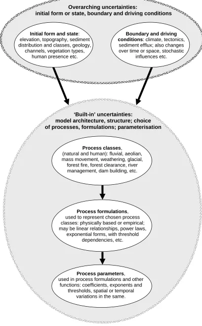
Figure 1.1: Main sources of uncertainty in LEMs and LEM studies (see text). Overarching uncertainties:
initial form or state, boundary and driving conditions
Process classes,
(natural and human): fluvial, aeolian, mass movement, weathering, glacial,
forest fire, forest clearance, river management, dam building, etc.
Process formulations, used to represent chosen process classes: physically based or empirical; may be linear relationships, power laws,
exponential forms, with threshold dependencies, etc.
Process parameters,
used in process formulations and other functions: coefficients, exponents and
thresholds, spatial or temporal variations in the same.
‘Built-in’ uncertainties:
model architecture, structure; choice of processes, formulations; parameterisation Initial form and state:
elevation, topography, sediment distribution and classes, geology,
channels, vegetation types, human presence etc.
Boundary and driving conditions: climate, tectonics,
sediment efflux; also changes over time or space, stochastic
In the figure, the uncertainties are shown as a hierarchy. Those relating to initial form or state, and to the boundary and driving conditions, are separated from those more closely associated with the ‘structure’ and ‘architecture’ of the LEM (these terms explained below). To begin with, as regards the initial form and the boundary and driving condition
uncertainties, these are seen as ‘overarching’, in that they are present whatever the LEM or LEMs being used, and often the main focus of the research. For example, if the study begins with a present day landscape, with the aim of understanding the effects of climate change, there will be errors in the DEM and other initialising data, and errors in the
projected climate itself, and also in the predicted vegetation succession and so on; similarly, if the LEM is used to understand the evolution of a landscape since a specified but distant past time, before historical records, then the initial landscape and its sediment cover will have to be hypothesised, and probably the climate and other driving conditions also to some extent, the uncertainties in the latter depending upon the availability and accuracy of past climate proxy data and related information.
By contrast with the overarching uncertainties, the ‘built-in’ uncertainties are seen largely as model dependent (e.g. Haff, 1996; Kirkby, 2000; Beven, 2002). More specifically, and for the purposes here, the term ‘model structure’ is intended to mean the theoretical
representation of the system itself, as signified by the things being modelled, in particular, the state variables and processes, and the links between them. Architecture, on the other hand, is intended to mean the manner in which that structure is arranged and divided for computational purposes, both over time and space. It follows that the same model structure might be represented by a range of different architectures; similarly, it could be possible for the same architecture to be used for discretisation of a range of different model structures. These matters are reviewed in more detail in Chapter 2.
It will be appreciated from this that built-in uncertainties are likely to be more or less fixed, in that there is little a researcher can do to change them or improve on them once a LEM has been selected, or built, for a research purpose. Admittedly, some LEMs permit a choice between different process classes or process formulations1, and others incorporate self-adjusting time steps and grid cell sizes (e.g. Braun and Sambridge, 1997; Coulthard et al., 1999), but this flexibility has to be limited, to keep model size and coding practical.
1
The hierarchical relationship between the built-in uncertainties is particularly evident in Figure 1.1. Specifically, the choice of process classes in a LEM will be strongly influenced by the climate being applied to the modelled landscape; for example, aeolian processes are not likely to be needed in simulations of humid environments, nor are nival processes likely to be needed in simulations of warm environments. Once the main process classes of interest have been chosen, process formulations will be needed to represent them, so the formulations employed will be stem from the process class choices. In this respect,
although past studies may guide a researcher which process formulation to prefer (assuming the LEM allows a choice), the matter is still subjective to some extent. In addition,
whichever formulation is chosen to represent a process or other LEM function, it will almost certainly not be wholly physically based, and must therefore be empirical in some respect (Thorn, 1988).
Continuing with the hierarchy, the process parameters required in the simulations follow inevitably from the selected process formulations. As explained above, the parameters are mostly empirical and of uncertain value. It should also be noted here, however, that as the number of different model functions increases, so too does the number of parameters needed to implement them (e.g. Beven, 1996; Kirkby, 1996). Whatever the other uncertainties, therefore, most LEMs have a large process parameter space, which comprises large dimensionality (the number of parameters) and value uncertainty (the combined ranges of acceptable value for each parameter). This is considered again at the end of Chapter 2, and the implications of large LEM parameter spaces on simulation work are reviewed in
Chapter 3.
appear to be small2, and vary in the simulation only those whose effects are greater, departing from this if the results appear problematical for some reason.
Having reviewed the main sources of uncertainty, the argument is now expanded to consider the associations between uncertainty, multiple working hypotheses and model equifinality.
Uncertainty, model equifinality and multiple working hypotheses
The discussion above outlines how the uncertainties in LEMs and LEM studies arise, both in the way LEMs are constructed and in the manner in which they are used. The difficulties posed by having such uncertainties become especially troublesome where LEMs are used to investigate inverse problems (e.g. Pollack, 2003), that is, where the aim is to explain the most likely evolution path of a present day landscape since a particular time in the past. If the model can be designed with a strong physical basis, e.g. as in geophysical research, then the main uncertainties in an inverse problem will be the initial state, the boundary and driving conditions, and the observation errors (ibid.). However, in LEMs, because of their semi-empirical basis, many of the built-in uncertainties cannot be avoided, and these uncertainties present any researcher with many possible variables. The term ‘variable’ is used here in a wide sense, namely to mean any factor, condition, parameter and so on, which may be altered at a researcher’s discretion, whether using just the one LEM, or more. With so many variables, LEM simulations can be run in many different ways (e.g. Beven, 1996; Kirkby, 2000). Moreover, this applies whether one is using just a single LEM, or if the aim is to contrast output from one LEM with another.
Why might this be a problem? The argument here is twofold. Firstly, given the general uncertainties, any simulation with a model will only be one of a number of possible explanations of reality (e.g. Freer et al., 1996; Beven and Freer, 2001; Helton, 2004; Oberkampf et al., 2004; Spear, 1997; and numerous others. See also Giere, 1999, and Pollack, 2003, for more philosophical discussions). Some of these will be better than others, however, in that their output closely resembles field or other relevant data to some degree, and out of these simulations, there may well be a selection generating the same or very similar output (Beven, 1996), thus demonstrating model equifinality.
2
Secondly, the use of LEMs can be likened to the demonstration of multiple working hypotheses (e.g. Platt, 1964; Haines-Young and Petch, 1983 and 1986; Schumm, 1991;
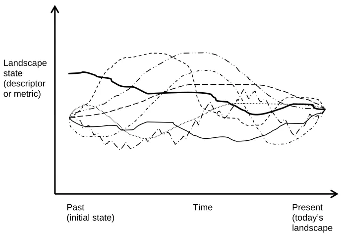
[image:29.595.132.475.292.519.2]Baker, 1996; Pollack, 2003; Inkpen, 2005). In this respect, each simulation with a LEM can be viewed as a working hypothesis in its own right, each aspect of the overarching and built-in uncertainties combining to form the overall hypothesis; likewise, a suite of different simulations can be treated as a set of such hypotheses. Where model equifinality occurs, however, the different evolution paths drawn by each simulation converge, and this makes falsification of any of the hypotheses problematic. Such a situation is shown graphically, in Figure 1.2, adapted from Church (2003).
Figure 1.2: LEM evolution paths represented as multiple working hypotheses (adapted from Church, 2003). The bold line represents the true evolution path of the landscape; the other
lines signify the evolution paths generated by different LEM simulations, each of which represents a different working hypothesis. In the figure, these are equifinal and converge on
the present state, which cannot alone be used as a measure to falsify any of the hypotheses.
In the figure, each working hypothesis relates to a simulation and is shown by its own ‘evolution path’ over time, this taken to be identified by some descriptor or metric of the landscape state. Whether the metric is simply a single property, such as the drainage
density, or a composite of different landscape properties, in the manner discussed by Church (2003), the path of the true landscape state over time is shown by the bold black line. This is assumed here to be the major unknown, and the target which the researcher is seeking to simulate.
Past (initial state) Landscape
state (descriptor or metric)
Ideally, all of the working hypotheses would be clearly distinguishable from each other, particularly in their final result, so that by the end of the simulations, any ‘wrong’
hypotheses would clearly differ from the real landscape (as measured by the descriptor or metric). In the Figure 1.2, however, model equifinality is present, and all of the
hypothesised evolution paths converge on the present state. In such a situation, the present state alone cannot be used to identify which evolution paths are wrong, and hence which of the multiple working hypotheses can be falsified.
[image:30.595.130.475.435.671.2]As discussed in subsection 1.2.1, the possibility arises of using more descriptors from the real landscape. In this way, equifinality to one descriptor may not be a problem if the model predictions are not equifinal for the others. However, there may still be difficulties caused by observation errors relating to the present day landscape, so that what constitutes an equifinal result itself becomes uncertain. If the simulations are run stochastically, using climate variations for example, the position may become yet more uncertain and blurred. Model equifinality to multiple measures therefore still presents potentially serious problems. As a variant of the situation pictured in Figure 1.2, Figure 1.3 shows model equifinality occurring where a common initial state is used for each LEM simulation.
Figure 1.3: LEM evolution paths represented as multiple working hypotheses (adapted from Church, 2003), but this time beginning with a common initial condition. As before, the bold
line represents the true evolution path of the landscape and the other lines signify the evolution paths generated by different LEM simulations. These are equifinal, so the measure
of the present state alone cannot be used to falsify any of the simulation hypotheses. Past
(initial state) Landscape
state (descriptor or metric)
In the figure, different system states emerge, as the evolution paths for each simulation at first diverge from each other. However, the paths converge later in the simulation, in this example all meeting at the present state of the real landscape. Presumably, variants and combinations of Figures 1.2 and 1.3 could be drawn, including representations with
observation and other errors. However, it will be appreciated that if the type of equifinality seen in Figure 1.3 can be shown to occur in LEMs, then that seen in Figure 1.2 must occur also3. It will also be appreciated from Figure 1.3 that even if a researcher happened to hypothesise the initial state correctly, so it coincided with the true initial state, then it would still not be possible from the final state alone to falsify the wrong hypotheses.
Researchers are probably well aware of the uncertainties in model studies, and of the latent difficulties posed by LEM equifinality. However, once the problem is understood in the terms states above, and despite the comments by some of the authors cited in the discussion, the potential for equifinality in LEM studies appears to be huge. If it is common, it implies that we cannot “… secure the survival of the fittest theory by the elimination of those which are less fit.” (Popper, 1969, page 313). We are also prevented from pursuing that “iterative back-and-forth interplay” between observations and models, which “… generally improves understanding of a system” (Pollack, 2003). Ubiquitous model equifinality in LEMs would therefore both obviate their use and frustrate progress in the discipline.
Given this conclusion, it clearly becomes necessary to consider how model equifinality can be dealt with. Although the problem appears difficult to manage, it may not be insuperable. In particular, if it can be assumed that LEM outputs are generally not due to inconsistencies in the calculating procedures or algorithms, nor to numerical instabilities of some kind, then they must represent a response to the model variables, manifested through their influence on the modelled landscape. As can be seen from Figure 1.1, these variables may stem from any of the sources of uncertainty in LEM studies. By examining LEM output for the influences of these variables, it should be possible to clarify whether equifinality does indeed occur, and the variables most likely to cause it. In addition, it may be possible to express the responses mathematically, thus clarifying how each variable affects model equifinality. An important preliminary step, therefore, before formulating the research aims, is to consider the range of variables used in LEM studies, and to examine their influence on LEM output. These matters are now briefly reviewed.
3
1.3 VARIABLES USED IN LEMS AND THEIR INFLUENCE ON OUTPUT
1.3.1 Table of example LEM studies
Table layout
To review all the findings of researchers who have used LEMs is a near impossible task, such has been the rate of increase in the use of LEMs over the last twenty years. The author has therefore taken examples from the literature to demonstrate the range of topics in geomorphology to which LEMs have been applied, and these are summarised in Table 1. The table also includes some studies with numerical slope evolution models, as these models work in an equivalent way to LEMs, and indications of equifinality in such studies would indicate that similar results in LEM studies are possible.
The table is divided into columns so as to distinguish between the simulation scenarios and variables, listed in column 2, and the main influences exhibited in the simulations, listed in column 3. The information in column 2 also highlights both the relative frequency of certain research themes in LEM studies generally, and the main variables of interest used in each of the listed studies. The information in column 3 is a summary of the results from each study, thus allowing variables and results to be seen side by side. It should be noted, however, that in summarising model results in column 3, the author’s focus on influences of the variables gives the results a different emphasis to that given to them by the original authors. This is deliberate, for the purposes of introducing the equifinality problem, and is not meant to detract in any way from the work as it was originally reported. Another difference from the original papers is that each study is summarised in terms of the
‘influences’ of the variables, rather than their ‘effects’. This is also deliberate, as the term ‘effect’ is used in a specific way in this thesis, particularly from Chapter 3 onwards, and this is rather different from the way effects are commonly described in LEM studies. Finally, before turning to the particular variables and influences listed in the table, it is also helpful to comment on the temporal focus of the studies and certain aspects of the presentation. For convenience here, references are cited by using the reference numbers in the table
Table 1: Examples of studies with LEMs and slope evolution models, summarising the main variables and their influence on model output.
Reference Main variables or scenario Main influences on results 1. Ahnert (1987) Process rate parameter values,
geology
Differences in balance between processes and rates at different places strongly influences resulting forms.
2. Armstrong (1987) Different initial slope forms, process classes and rates, rates of basal removal
Large differences in the initial form have a strong influence on the evolution of transient slope forms.
Combinations of different processes can produce very similar transient forms, suggesting equifinality and convergence. Low weathering rates limit erosion and strongly influences slope form evolution; high rates have little or no influence. Rate of basal removal influences eventual slope forms and the depth of lower slope sediments.
Different erosion processes produce different patterns of deposition on lower slopes, whatever the eventual slope form. 3. Bogaart et al. (2003a) Climate and process parameters Climate strongly influences surface runoff generation, areas draining into channel heads, and sediment yield.
Change of climate from cold to warm reduces sediment yield.
Change of climate from warm to cold increases drainage density, and sediment yield until ready supplies are exhausted. 4. Bogaart et al. (2003b) Climate and process parameters Variables have a strong influence on hillslope erosion, fluvial sediment transport, deposition and related output measures.
Strength of influences changes over time. 5. Braun & Sambridge
(1997)
Cell geometries, size and number Cell grid scheme influences routing of channels and sediment, sinuosity, drainage density, and over time, topography. 6. Clevis et al. (2003) Bedrock erodibility, rate of thrust
displacement, temporal tectonic and sea level (base level) fluctuations
Bedrock erodibility strongly influences sedimentation rates, although effect changes over time.
7. Coulthard & Macklin (2005)
Different study sites, same long term general climate signals per site
Shifts to a wetter climate have a strong and almost immediate influence on sediment yield from the catchment as a whole. Land cover (forest) influences peaks in the sediment yield in response to the same climate conditions.
Pattern of sediment movement within catchments is strongly determined by location.
Responses over time of erosion and sedimentation to the same climate forcing are ‘noisy’, with possible pulsations. 8. De Boer (2001) Rainstorm area in inverse relation
to rainstorm frequency
Frequency of rainstorms strongly influences the total sediment yield from the basin. (Note 1.)
Area of storms influences the sediment yield, whereas position of storms influences the formation of relief and topography. 9. Fagherazzi et al.
(2004)
Sea level oscillations, climate (runoff), initial topography
Oscillation amplitude of sea level change strongly influences river mouth incision.
Small amplitude oscillations in sea level have little influence on lowering of river beds, whereas larger amplitude oscillations have a stronger influence, causing the formation of knickpoints that propagate upstream.
Climate (via as an increase in runoff) strongly influences formation of new incisions and sediment delivery to the shelf. Initial topography strongly affects position of initial channels and subsequent development of channels and topography. 10. Fischer et al. (2004) Uplift and tectonic rebound coupled
to a surface process model (LEM)
Fluvial removal processes, rebound and base level changes together strongly influence formation of realistic relief.
11. Gargani et al. (2006) Long term climate shifts, base level Pattern of climate change strong affects sediment yield and fluvial erosion.
Base level changes have little influence on fluvial erosion at certain stages of the climate cycle. 12. Gasparini et al.
(1999)
Runoff, sediment classes and proportions thereof
Variations in runoff, slope and sediment characteristics influence downstream fining in eroding networks.
Initial proportions of sediment classes have little influence on pattern of downstream fining that eventually emerges. 13. Gasparini et al.
(2004)
Climate, uplift, grain sizes and mixing again
Sediment grain size strongly affects channel concavity and relief.
Table 1 (cntd): Examples of studies with LEMs and slope evolution models, summarising the main variables and their influence on model output.
Reference Main variables or scenario Main influences on results 14. Hancock (2003) Erosion parameters, catchment
aspect ratio
Erosion parameters and aspect ratio both influence hypsometric curve, area-slope relationship, channel width function and cumulative area distribution, although influence of some parameters/variations is greater than others.
15. Howard (1994) Uplift and climate scenarios, and different erosion law formulations
Form of fluvial erosion law has strong influence, in the presence of uplift, on locations and rates of stream erosion in transient landscapes
16. Kirkby (1989) Different climatic conditions, initial forms, time periods, process classes and process rate parameters, land management systems
Combinations of land management practices and climate strongly influence the evolution of slopes and sediment profiles. Responses to different temperature, hydrology, land cover and weathering are made more complex depending upon type of main climate being applied.
Influence of new climate or new land use on an otherwise near-stable soil profile may be strong and non-linear 17. Kooi & Beaumont
(1996)
Forms of process law; also uplift and transport/erosion rates
Response time of the landscape (as determined by process rate coefficients, laws and so on) and tectonics have important influences on patterns of landscape evolution.
18. Lancaster et al. (2001)
Numerous process parameters and site variables, including woody debris supply
Debris dams have little influence on sediment yield from a catchment, but absence of dams or a low supply of wood strongly influences the degree of pulsing of sediment through the system and the formation of terraces.
Combined influences of debris flows, wood supply and in-channel sediment storage may be complex and counter-intuitive. 19. Martin (2000) Weathering rates, diffusivities,
process formulations
Weathering strongly influences transport by mass movement on steep slopes, low rates limiting erosion by creep and slides. Diffusivities (incorporating both creep and slide) strongly influence slope forms, subject to limiting weathering rates. 20. Moglen & Bras
(1995)
Soil erodibility, expressed as ‘softness’
Variability in soil ‘softness’ strongly affects sinuosity and convex-concave slope variability.
Vertical variation strongly affects shape of hypsometric curve, whereas horizontal variation strongly influences relief. 21. Niemann et al.
(2001)
Uplift Uplift rates strongly affect the vertical migration rates of knickpoints. 22. Rinaldo et al. (1995) Cyclic variation in τc (surface
resistance), to effect climate change
Change in climate over time has complex (lagged) influences on drainage density, valley density and (fractal) topography. Evidence of past climates is complicated by uplift, slope-dependent processes and amplitude of the changes. (Note 2) 23. Rosenbloom &
Anderson (1994)
Diffusivities, weathering, forms of process law, stream incision parameter
Hillslope diffusivity rates have a strong influence on evolution of realistic forms. Weathering rates have little influence on slope evolution unless they are low and limiting. Stream incision parameter has a strong influence on the stream profile.
24. Schlunegger et al.
(2001)
Climate and geology, tectonic response to unloading following erosion
Change in climate strongly influences erosion and sediment yield; sediment yield also changes with time. Different geologies/strata strongly influence re-routing of drainage network.
Tectonic response to erosion (unloading) influences re-routing of channels, drainage density and sediment yield. 25. Tucker (2004) Climate and uplift, use of threshold
law
Over long time scales, absence of a threshold has a strong effect on pattern of slope retreat
A threshold in the erosion-transport laws strongly influences scarp evolution response to tectonic and climate forcing. Influence of the erosion threshold appears to be greater where fewer than 50% of flood events can mobilise sediment. 26. Tucker & Bras
(1998)
Contrasts between different process classes and formulations
Different process classes and formulations have strong but different influences on landscapes and produce different equilibrium or final forms.
27. Tucker & Bras (2000)
Short term climate – intensity, frequency, variability
[image:34.595.70.790.127.509.2]Table 1 (cntd): Examples of studies with LEMs and slope evolution models, summarising the main variables and their influence on model output.
Reference Main variables or scenario Main influences on results 28. Tucker &
Slingerland (1994)
Process classes and formulations, uplift, initial forms, process rate parameters
Different process formulations strongly affect characteristic evolution of the landscape and drainage system, particularly where the weathering rate is limiting.
The slope failure angle and bedrock erodibility strongly influence the pattern of scarp retreat.
Uplift and rebound help to maintain steeper channel gradients and hillslopes near the highest part of the escarpment. 29. Tucker &
Slingerland (1996)
Uplift scenarios, variable geology (bedrock erodibility functions)
Variable geology strongly influences sediment yields, drainage density, patterns of erosion and sedimentation within the basin or range, and consequently affects the evolution of relief; uplift and rebound exert additional influences.
30. Tucker & Slingerland (1997)
Changes in intensity of runoff, overall runoff and erosion threshold (τc).
Runoff intensity strongly influences erosion, deposition, channel heads, drainage density, and hillslope gradients over time. Change in erosion threshold also influences the above, but less markedly than changes in runoff intensity.
Weathering and sediment supply to channels exert a limiting influence under some climate conditions. 31. Tucker & Whipple
(2002)
Influence of slope exponent in detachment-limited erosion law
Value of slope exponent in detachment-limited stream erosion law strongly influences form of slope retreat, rates and locations of erosion, positions of knickpoints and eventual slope profiles.
32. Whipple & Tucker (1999)
Uplift rate, ratio of m/n in stream erosion law.
Ratio of m/n has a strong influence on relationship between elevation and distance from the divide in equilibrium forms. Slope exponent n and uplift rate together have strong influence on response time of landscape to sudden base level changes. 33. Willgoose (1994a) Contrast dynamic and declining
equilibrium (rate of base level change)
Rate of uplift determines slope-area relationship as the landscape approaches dynamic equilibrium or declining relief. Area and slope exponents (m and n) in transport laws also influence the area-slope relationship and the position in the curve indicating where dominance shifts from diffusive (hillslope) to fluvial processes.
34. Willgoose (1994b) Uplift rates, including step changes; also climate
Slope-area relationship is sensitive in different ways to various uplift and climate change combinations, some of these combinations influencing the form of the curve more strongly than others.
35. Willgoose et al. (1991c)
Uplift and climate; also process parameters.
Balance between diffusive and fluvial processes strongly influences form of the area-slope relationship under dynamic equilibrium. Transient influences also noted.
36. Willgoose et al. (1991d)
Implemented distinct channels, contrasted different channel formation rules and influence of perturbations in initial landscape
Distinct channels influence sediment routing and evolution of morphology.
Perturbations in initial landscape (elevation) strongly influence channel location and direction along which they extend. If fluvial processes are dominant, then increasing aridity has little influence on non-dimensional form of landscape, whereas if diffusive processes are dominant, then combinations of different uplift and diffusivity may produce similar,
non-dimensional landscape forms. 37. Willgoose and
Hancock (1998)
Uplift, process parameters High diffusivities have a strong influence on the shape of the hypsometric curve in steady state or declining relief landscapes, whereas lower diffusivities have little influence.
The aspect ratio influences the hypsometric curve in steady state landscapes.
Subtler, more detailed influences of the erosion process exponents m and n also noted. 38. Willgoose et al.
(2003)
Different parameter values and output metrics
Influences of different parameter values on a single output metric are too small to allow its sole use as a calibration measure, and the use of suites of output statistics is recommended in calibration work. (Note 3)
Notes:
1. De Boer applied a rule whereby the frequency of a storm of a particular size was inversely related to its area.
[image:35.595.72.772.125.494.2]