On Long Term Climate Studies Using a Coupled General Circulation Model

The CSIRO Mk3L climate

system model

2.1

Introduction

The CSIRO Mk3L climate system model comprises two components: an atmospheric general circulation model, which incorporates both a sea ice model and a land sur-face model, and an oceanic general circulation model. The atmospheric general circulation model is a low-resolution version of the atmospheric component of the CSIRO Mk3 coupled model (Gordon et al., 2002), while the oceanic general circu-lation model is the oceanic component of the CSIRO Mk2 coupled model (Gordon and O’Farrell, 1997).

This combination takes advantage of the rapid execution times of the Mk2 cou-pled model, which result from the low horizontal resolution, while also taking ad-vantage of the enhanced physics of the Mk3 atmosphere model. Relative to the Mk2 atmosphere model, enhancements to the physics include:

• _{an increase in the vertical resolution from 9 to 18 levels}

• _{the incorporation of a prognostic scheme for stratiform cloud}

• _{the incorporation of a new cumulus convection scheme}

• _{an enhanced land surface model}

The development of Mk3L from these components is described in detail byPhipps (2006). The resulting model is computationally efficient, portable across a wide range of computer architectures, and suitable for studying climate variability and change on millennial timescales.

The model physics is described in Section 2.2, while Section 2.3 outlines the spin-up procedure. The ability of the atmospheric and oceanic components to simulate the present-day climate is evaluated in Sections 2.4 and 2.5 respectively, and the flux adjustments required by the coupled model are derived in Section 2.6.

The material presented in Section 2.2 also appears in Phipps (2006), but is reproduced here in the interests of completeness.

2.2

Model description

2.2.1 Atmosphere model

The CSIRO Mk3 atmosphere model consists of three components: an atmospheric general circulation model, a multi-layer dynamic-thermodynamic sea ice model and a land surface model. As each of these components is documented in detail byGordon et al. (2002), only a brief summary is provided here. This summary concentrates on those features which are unique to Mk3L, and on those which are particularly relevant to this project.

The standard configuration of the Mk3 atmosphere model employs a spectral resolution of T63. However, a spectral resolution of R21 is also supported for re-search purposes, and it is this resolution which is used within Mk3L. The zonal and meridional resolutions are therefore 5.625◦ _{and ∼3.18}◦ _{respectively.}

Atmospheric general circulation model

The dynamical core of the atmosphere model is based upon the spectral method, and uses the flux form of the dynamical equations (Gordon, 1981). Physical pa-rameterisations and non-linear dynamical flux terms are calculated on a latitude-longitude grid, with Fast Fourier Transforms used to transform fields between their spectral and gridded forms. Semi-Lagrangian transport is used to advect moisture (McGregor, 1993), and gravity wave drag is parameterised using the formulation of Chouinard et al. (1986).

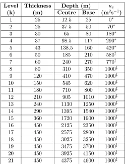
A hybrid vertical coordinate is used, which is denoted as theη-coordinate. The Earth’s surface forms the first coordinate surface, as in the σ-system, while the remaining coordinate surfaces gradually revert to isobaric levels with increasing altitude. The 18 vertical levels used in the Mk3L atmosphere model are listed in Table 2.1 (Gordon et al., 2002, Table 1).

The topography is derived by interpolating the 1◦_×1◦ _{dataset of Gates and}

Nelson (1975a) onto the model grid. Some modifications are then made, in order to avoid areas of significant negative elevation upon fitting to the (truncated) resolution of the spectral model (Gordon et al., 2002). The resulting topography is shown in Figure 2.1.

Time integration is via a semi-implicit leapfrog scheme, with a Robert-Asselin time filter (Robert, 1966) used to prevent decoupling of the time-integrated solutions at odd and even timsteps. The Mk3L atmosphere model uses a timestep of 20 minutes.

The radiation scheme treats solar (shortwave) and terrestrial (longwave) radi-ation independently. Full radiradi-ation calculradi-ations are conducted every two hours, allowing for both the annual and diurnal cycles. Clear-sky radiation calculations are also performed at each radiation timestep. This enables the cloud radiative forcings to be determined using Method II ofCess and Potter (1987), with the forc-ings being given by the differences between the radiative fluxes calculated with and without the effects of clouds.

Level η Approximate

(k) height (m)

18 0.0045 36355 17 0.0216 27360 16 0.0542 20600 15 0.1001 16550 14 0.1574 13650 13 0.2239 11360 12 0.2977 9440 11 0.3765 7780 10 0.4585 6335 9 0.5415 5070 8 0.6235 3970 7 0.7023 3025 6 0.7761 2215 5 0.8426 1535 4 0.8999 990 3 0.9458 575 2 0.9784 300 1 0.9955 165

Table 2.1: The hybrid vertical levels used within the Mk3L atmosphere model: the value of theη-coordinate, and the approximate height (m).

bands, the radiative properties are taken as being uniform. Ozone concentrations are taken from the AMIP II recommended dataset (Wang et al., 1995). Additional code has been inserted into Mk3L, enabling both the solar constant and the epoch to be specified at runtime, with the Earth’s orbital parameters being calculated by the model (Phipps, 2006).

The longwave radiation scheme uses the parameterisation developed by Fels and Schwarzkopf (Fels and Schwarzkopf, 1975, 1981;Schwarzkopf and Fels, 1985, 1991), which divides the longwave spectrum (wavelengths longer than 5 µm) into seven bands. Values for the CO2 transmission coefficients must be provided at runtime.

The cumulus convection scheme is based on the U.K. Meteorological Office scheme (Gregory and Rowntree, 1990), and generates both the amount and the liquid water content of convective clouds. This scheme is coupled to the prognostic cloud scheme ofRotstayn (1997, 1998, 2000), which calculates the amount of strati-form cloud, using the three prognostic variables of water vapour mixing ratio, cloud liquid water mixing ratio and cloud ice mixing ratio.

In the stand-alone atmosphere model, four types of surface gridpoint are em-ployed: land, sea, mixed-layer ocean and sea ice. The temperatures of the sea gridpoints are determined from monthly observed sea surface temperatures, which must be provided at runtime. Linear interpolaton in time is used to estimate values at each timestep, with no allowance for any diurnal variation. At high latitudes, sea gridpoints may be converted to mixed-layer ocean gridpoints, with self-computed temperatures; these can then evolve into sea ice gridpoints. This is discussed further in the following description of the sea ice model.

Sea ice model

The sea ice model includes both ice dynamics and ice thermodynamics, and is de-scribed by O’Farrell (1998). Internal resistance to deformation is parameterised using the cavitating fluid rheology of Flato and Hibler (1990, 1992). The thermo-dynamic component is based on the model of Semtner (1976), which splits the ice into three layers, one for snow and two for ice. Sea ice gridpoints are allowed to have fractional ice cover, representing the presence of leads and polynyas.

Ice advection arises from the forcing from above by atmospheric wind stresses, and from below by oceanic currents. The currents are obtained from the ocean model when running as part of the coupled model; in the stand-alone atmosphere model, climatological ocean currents must be provided.

The advance and retreat of the ice edge in the stand-alone atmosphere model is controlled by using a mixed-layer ocean to compute water temperatures for those sea gridpoints which lie adjacent to sea ice. The mixed-layer ocean has a fixed depth of 100 m, and the evolution of the water temperature Ts is calculated using

the surface heat flux terms and a weak relaxation towards the prescribed sea surface temperatureTSST, as follows (Gordon et al., 2002, Equation 19.6):

γ0

dTs

dt = (1−αs)S

↓

s +R↓s−ǫsσTs4−(Hs+Es) +λc(TSST −Ts) (2.1)

Here, γ0 represents the areal heat capacity of a 100 m-thick layer of water,

downward surface fluxes of shortwave and longwave radiation respectively, ǫs

repre-sents the surface emissivity, σrepresents the Stefan-Boltzmann constant,HsandEs

represent the net upward surface fluxes of sensible and latent heat respectively, and λc represents a relaxation constant. Mk3L uses a relaxation timescale of 23 days.

A mixed-layer ocean gridpoint can become a sea ice gridpoint either when its temperature falls below the freezing point of seawater, which is taken as being -1.85◦_{C, or when ice is advected from an adjacent sea ice gridpoint. When a}

mixed-layer ocean gridpoint is converted to a sea ice gridpoint, the initial ice concentration is set at 4%. The neighbouring equatorward gridpoint, if it is a sea gridpoint, is then converted to a mixed-layer ocean gridpoint.

Within a gridpoint that has fractional sea ice cover, both in the stand-alone atmosphere model and the coupled model, the water temperature is calculated using a mixed-layer ocean with a fixed depth of 100 m. The surface heat flux is given by Equation 2.1, except that the final relaxation term is replaced with a basal heat flux Fi, which is calculated as follows (Gordon et al., 2002, Equation 19.8):

Fi=

kfrzρwcwdz(TSST −Tf)

(dz/2)2 +Fgeog (2.2)

Here, kfrz = 0.15×10−4 s−1 is the heat transfer coefficient, ρw and cw are the

density and specific heat capacity of seawater respectively,dz= 25 m is the thickness of the upper layer of the ocean model, andTf = -1.85◦C represents the freezing point

of seawater. TSST represents the prescribed sea surface temperature in the case of

the stand-alone atmosphere model, and the temperature of the upper level of the ocean in the case of the coupled model. The additional fixed componentFgeog allows

for the effects of sub-gridscale mixing. Its value is resolution-dependent and, at the horizontal resolution of R21 used in Mk3L, is equal to 2 Wm−2

in the Northern Hemisphere, and 15 Wm−2

in the Southern Hemisphere.

If, within the coupled model, the temperature of the upper level of the ocean TOC falls below -2◦C, an additional term is added to the ice-ocean heat flux, as

follows (Gordon et al., 2002, Equation 19.9):

Ffrz =

kfrzρwcwdz(TOC−Tf)

(dz/2)2 (2.3)

In this case,kfrz is increased to 6×10−4 s−1 in order to stimulate the formation

of sea ice in sub-freezing waters.

Surface processes can lead to either a decrease in ice volume, as a result of either melting or sublimation, or an increase in ice volume; this can occur either when the depth of snow exceeds 2 m, in which case the excess is converted into an equivalent amount of ice, or when the weight of snow becomes so great that the floe becomes completely submerged. When the latter occurs, any submerged snow is converted into “white” ice.

Lateral and basal ice growth and melt are determined by the temperature of the mixed-layer ocean. Additional ice can grow when the water temperature falls below the freezing point of seawater, -1.85◦_{C, subject to a maximum allowable thickness of}

6 m. Once the water temperature rises above -1.5◦_{C, half of any additional heating}

to melt ice. In the case of the stand-alone atmosphere model, a sea ice gridpoint is converted back to a mixed-layer ocean gridpoint once the sea ice has disappeared. The neighbouring equatorward gridpoint, if it is a mixed-layer ocean gridpoint, is then converted back to a sea gridpoint.

Land surface model

The land surface model is an enhanced version of the soil-canopy scheme of Kowal-czyk et al. (1991, 1994). A new parameterisation of soil moisture and temperature has been implemented, a greater number of soil and vegetation types are available, and a multi-layer snow cover scheme has been incorporated.

The soil-canopy scheme allows for 13 land surface and/or vegetation types and nine soil types. The land surface properties are pre-determined, with seasonally-varying values being provided for the albedo and roughness length, and annual-mean values for the vegetation fraction. The stomatal resistance is calculated by the model, as are seasonally-varying vegetation fractions for some vegetation types. The soil model has six layers, each of which has a pre-set thickness. Soil temper-ature and the liquid water and ice contents are calculated as prognostic variables. Run-off occurs once the surface layer becomes saturated, and is assumed to travel instantaneously to the ocean via the path of steepest descent.

The snow model computes the temperature, snow density and thickness of three snowpack layers, and calculates the snow albedo. The maximum snow depth is set at 4 m (equivalent to 0.4 m of water).

2.2.2 Ocean model

The CSIRO Mk2 ocean model is a coarse-resolution, z-coordinate general circula-tion model, based on the implementacircula-tion by Cox (1984) of the primitive equation numerical model of Bryan (1969). It is described byGordon and O’Farrell (1997) and Hirst et al. (2000) and, with some slight modifications to the physics, by Bi (2002).

The prognostic variables used by the model are potential temperature, salinity, and the zonal and meridional components of the horizontal velocity. The Arakawa B-grid (Arakawa and Lamb, 1977) is used, in which the tracer gridpoints are located at the centres of the gridboxes, and the horizontal velocity gridpoints are located at the corners. The vertical velocity is diagnosed through application of the continuity equation.

The horizontal grid matches the Gaussian grid of the atmosphere model, such that the tracer gridpoints on the ocean model grid coincide with the gridpoints on the atmosphere model grid. The zonal and meridional resolutions are therefore 5.625◦ _{and ∼3.18}◦ _{respectively. There are 21 vertical levels, which are listed in}

Table 2.2.

The bottom topography is derived by interpolating the 1◦_×1◦ _{dataset of Gates}

Level Thickness Depth (m) κe

(k) (m) Centre Base (m2

s−1 )

1 25 12.5 25 0∗

2 25 37.5 50 70∗

3 30 65 80 180∗

4 37 98.5 117 290∗

5 43 138.5 160 420∗

6 50 185 210 580†

7 60 240 270 770†

8 80 310 350 1000‡

9 120 410 470 1000‡

10 150 545 620 1000‡

11 180 710 800 1000‡

12 210 905 1010 1000‡

13 240 1130 1250 1000‡

14 290 1395 1540 1000‡

15 360 1720 1900 1000‡

16 450 2125 2350 1000‡

17 450 2575 2800 1000‡

18 450 3025 3250 1000‡

19 450 3475 3700 1000‡

20 450 3925 4150 1000‡

21 450 4375 4600 1000‡

Table 2.2: The vertical levels used within the Mk3L ocean model: the thickness, the depth of the centre and base of each gridbox, and the value of the isopycnal thickness diffusivity. ∗_{These values are hard-coded into the model.} †_{These values}

are the maximum allowable values, and are hard-coded into the model; lower values may be specified via the model control file. ‡These values are specified via the model control file, and represent the values used for this project.

A number of changes are made to the land/sea mask, relative to the atmosphere model. The land gridpoints at the tips of South America and the Antarctic Penin-sula are replaced with ocean gridpoints, ensuring that Drake Passage accommodates three horizontal velocity gridpoints. In order to ensure adequate resolution of the Greenland-Scotland sill, Iceland is removed; likewise, adequate resolution of the flows through the Indonesian archipelago is ensured through a number of modifica-tions to the land/sea mask.

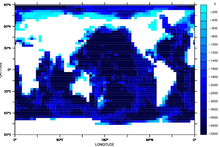
Figure 2.2: The bathymetry of the Mk3L ocean model: the depth of ocean gridpoints (m).

As a result of these changes, there are just four landmasses on the ocean model grid:

• _{Europe/Africa/Asia/North America/South America/Greenland}

• _Antarctica

• _{Australia/New Guinea}

• _{New Zealand}

The only other modifications to the land/sea mask are to the Hudson and Gibral-tar Straits, which are too narrow on the model grid to contain any horizontal velocity gridpoints; these straits are therefore closed.

The consolidation of the Earth’s land surface into four landmasses improves the computational performance of the ocean model. This is a consequence of the rigid-lid boundary condition (Cox, 1984), which is employed in order to remove the timestep limitation associated with high-speed external gravity waves. Under this boundary condition, the external mode of momentum is represented by a volume transport streamfunction,ψ:

u = − 1 aH

∂ψ

∂φ (2.4)

v = 1 aHcosφ

∂ψ

Here, u and v represent the zonal and meridional components, respectively, of the vertically-averaged velocity, arepresents the radius of the Earth,H represents the depth of the ocean, and φand λrepresent latitude and longitude respectively. At lateral walls, the boundary conditions on u and v are

u=v = 0 (2.6)

The boundary condition on ψat lateral walls is therefore

∂ψ ∂φ =

∂ψ

∂λ = 0 (2.7)

This condition is satisfied by setting ψ constant along the boundary of each unconnected landmass. If islands are present, the constant value of ψ for each island indicates the net flow around that island, and hence must be predicted by the governing equations. The method used in the ocean model is hole relaxation, in which the line integral of the quantity ∇_{psurface, where psurface is the surface} pressure, around each island is required to vanish.

By consolidating the Earth’s land surface into four landmasses, and by setting the net flow around Europe-Africa-Asia-North America-South America-Greenland equal to zero, it is only necessary to calculate the line integrals around three rela-tively small islands (Antarctica, Australia-New Guinea and New Zealand).

The bathymetry of the Mk3L ocean model defines six basins which have no resolved connection with the world ocean: the Baltic, Black, Caspian and Mediter-ranean Seas, Hudson Bay and the Persian Gulf. It does not therefore adequately represent the physical connections which exist within the ocean; with the exception of the Caspian Sea, each of these basins exchanges water with the world ocean via straits which are not resolved on the model grid. The effects of these exchanges are parameterised within the model through an imposed mixing between the gridpoints which lie to either side of each unresolved strait. This mixing has been substantially improved in Mk3L (Phipps, 2006).

Time integration is via a leapfrog scheme, with mixing timesteps conducted once every 19 tracer timesteps in order to prevent decoupling of the time-integrated solutions at odd and even timesteps. Fourier filtering is used to reduce the timestep limitation arising from the CFL criterion (e.g. Washington and Parkinson, 1986) associated with the convergence of meridians at high latitudes, particularly in the Arctic Ocean (Cox, 1984). In the Mk3L ocean model, Fourier filtering is only applied northward of 79.6◦_{N in the case of tracers, and northward of 81.2}◦_{N in the case of}

horizontal velocities (Phipps, 2006). The ocean bottom is assumed to be insulating, while no-slip and insulating boundary conditions are applied at lateral boundaries. The stand-alone ocean model employs an asynchronous timestepping scheme, with a timestep of 1 day used to integrate the tracer equations and a timestep of 20 minutes used to integrate the momentum equations. Within the coupled model - and during the final stage of spin-up runs, prior to coupling to the atmosphere model - a synchronous timestepping scheme is employed, with a timestep of 1 hour used to integrate both the tracer and momentum equations.

The vertical diffusivity κv varies as the inverse of the Brunt-V¨ais¨al¨a

at 3×₁₀−5 _m2_s−1_{, except in the upper levels of the ocean, where it is increased in} order to simulate the effects of mixing induced by surface winds. The minimum diffusivity between the upper two levels of the model is set at 2×₁₀−3 _m2_s−1_{, while} that between the second and third levels is set at 1.5×₁₀−4

m2

s−1

. Whenever static instability arises, the vertical diffusivity is increased to 100 m2

s−1

, simulating con-vective mixing.

Two parameterisations are incorporated in order to represent the mixing along isopycnal surfaces (i.e. surfaces of constant density). The first of these parameter-isations is the isopycnal diffusion scheme of Cox (1987), which allows for a more realistic representation of the tendency for tracers to be mixed along surfaces of constant density. For this project, the isopycnal diffusivity was set to the depth-independent value of 1000 m2

s−1

.

The second parameterisation is the scheme of Gent and McWilliams (1990) and Gent et al. (1995), which parameterises the adiabatic transport of tracers by mesoscale eddies. An eddy-induced horizontal transport velocity is diagnosed, which is added to the resolved large-scale horizontal velocity to give an effective horizon-tal transport velocity. The continuity equation can be used to derive the vertical component of either the eddy-induced transport velocity or the effective transport velocity. In Mk3L, Gent-McWilliams eddy diffusion is employed at all latitudes; previously there was a transition to horizontal diffusion within the Arctic Ocean (Phipps, 2006).

Previous studies (e.g.Hirst and McDougall, 1996;England and Hirst, 1997;Hirst and McDougall, 1998) have found significant improvements in the ocean climate, particularly in the Southern Ocean, upon incorporation of Gent-McWilliams eddy diffusion into their implementations of the Bryan-Cox ocean model. These improve-ments include: more realistic deep water properties; a substantial reduction in the amount of convective overturning in the Southern Ocean; a corresponding reduc-tion in the magnitude of the implied surface fluxes in the Southern Ocean; and a more realistic meridional overturning circulation. Furthermore, it was found that it was possible to remove the non-physical horizontal diffusivity that had previously been required to suppress numerical noise, and yet which significantly distorted the ocean climate though the production of large and spurious horizontal diffusive fluxes. Further studies byHirst et al. (1996, 2000) found that the incorporation of Gent-McWilliams eddy diffusion into the oceanic component of a coupled general circulation model reduced the magnitude of the flux adjustments required in the Southern Ocean, and virtually eliminated the drift that was previously found to occur.

The values for the isopycnal thickness diffusivity which were used for this project are shown in Table 2.2. Notewhich that the values for levels 1 to 5 are fixed, and are hard-coded into the model. The values for levels 6 and 7 are maximum values, and these upper limits are also hard-coded into the model. Smaller values may be specified via the model control file, but the diffusivity may not exceed 580 and 770 m2

s−1

In the stand-alone ocean model, monthly values must be provided for the sea surface temperature (SST), sea surface salinity (SSS), and the zonal and meridional components of the surface wind stress. Linear interpolation in time is used to estimate values at each timestep. The temperature and salinity of the upper layer of the model are relaxed towards the prescribed SST and SSS, using a default relaxation timescale of 20 days. In Mk3L, it is possible for a different relaxation timescale to be specified via the model control file (Phipps, 2006).

2.2.3 Coupled model

The coupling between the atmosphere model (AGCM) and ocean model (OGCM) has been modified in Mk3L, in order to ensure that heat and freshwater are rigor-ously conserved (Phipps, 2006). Within the Mk3L coupled model, four fields are passed from the AGCM to the OGCM: the surface heat flux, surface salinity ten-dency, and the zonal and meridional components of the surface momentum flux. Four fields are also passed from the OGCM to the AGCM: the sea surface temper-ature (SST), sea surface salinity (SSS), and the zonal and meridional components of the surface velocity.

The Mk3L coupled model runs in a synchronous mode, with one OGCM timestep (1 hour) being followed by three AGCM timesteps (3 ×_{20 minutes). The surface} fluxes calculated by the AGCM are averaged over the three consecutive AGCM timesteps, before being passed to the ocean model.

In the case of the surface fields passed from the OGCM to the AGCM, instan-taneous values for the zonal and meridional components of the surface velocity are passed to the AGCM. These velocities act as the bottom boundary condition on the sea ice model for the following three AGCM timesteps. In the case of the SST and SSS, however, the OGCM passes two copies of each field: one containing the values at the current OGCM timestep, and one containing the values which have been predicted for the next OGCM timestep. The AGCM then uses linear interpolation in time to estimate the SST and SSS at each AGCM timestep.

Flux adjustments are applied to each of the fluxes passed from the AGCM to the OGCM, and also to the SST and SSS. The need to apply adjustments to the surface velocities is avoided by using climatological values, diagnosed from an OGCM spin-up run, to spin spin-up the AGCM.

2.3

Spin-up procedure

2.3.1 Atmosphere model

The atmosphere model was spun up for pre-industrial conditions, consistent with PMIP2 experimental design (Section A.2). The atmospheric carbon dioxide was set equal to 280 ppm, the solar constant was set equal to 1365 Wm−2

, and modern (AD 1950) values were used for the Earth’s orbital parameters.

Stage Boundary Timesteps Duration

conditions T, S ψ, u, v (years)

1 Annual means 1 day 20 minutes 1,000 2 Monthly means 1 day 20 minutes 3,000 3 Monthly means 1 hour 1 hour 500

Table 2.3: A summary of the spin-up procedure for the Mk3L ocean model.

from the final 100 years of the ocean model spin-up run (Section 2.3.2). Further information regarding the experimental design is provided in Appendix A.

The run was integrated for 50 years, and shall be referred to herein as A-DEF.

2.3.2 Ocean model

The spin-up procedure for the ocean model was essentially that of Gordon and O’Farrell (1997) and Bi (2002), and is summarised in Table 2.3.

The World Ocean Atlas 1998 dataset (National Oceanographic Data Center, 2002) was used to initialise the model, in accordance with PMIP2 experimental design (Section A.2). The model was forced with the NCEP-DOE Reanalysis 2 (Kanamitsu et al., 2002) wind stresses, while the temperature and salinity of the upper layer of the model were relaxed towards the World Ocean Atlas 1998 val-ues, using a relaxation timescale of 20 days. Further information regarding the experimental design is provided in Appendix A.

The model was initially integrated to equilibrium using asynchronous ping. This allows for a much longer tracer timestep than synchronous timestep-ping would impose (1 day, as opposed to 1 hour), thereby accelerating convergence towards an equilibrium solution. For the first 1,000 years, annual-mean surface boundary conditions were applied to the model, reducing the magnitude of the ini-tial surface fluxes and allowing for longer timesteps than would otherwise be possible. Monthly-mean surface boundary conditions were applied thereafter.

The convergence criteria were those of Bi (2002), with the ocean model be-ing regarded as havbe-ing attained equilibrium once the rates of change in global-mean temperature and salinity, at each model level, were less than 0.005◦_C/century

and 0.001 psu/century respectively. These criteria were found to be satisfied after 4,000 years of asynchronous timestepping.

The final stage of the spin-up employed synchronous timestepping, with a time-step of 1 hour used to integrate both the tracer and momentum equations. These are the same timesteps used within the coupled model, and this final stage therefore ensures no change in the ocean model configuration upon coupling to the atmosphere model. Although the aforementioned convergence criteria were satisfied after just 200 years, the model was integrated for a total of 500 years under synchronous time-stepping. This created an extended period from which an ocean model climatology could be derived, while also ensuring that any residual drift was negligible.

Between the penultimate and final centuries of the run, the changes in global-mean temperature and salinity did not exceed 1.9×10−3◦_{C and 1.8×10}−4

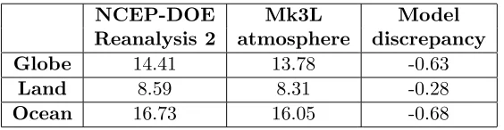
NCEP-DOE Mk3L Model Reanalysis 2 atmosphere discrepancy

Globe 14.41 13.78 -0.63

Land 8.59 8.31 -0.28

Ocean 16.73 16.05 -0.68

Table 2.4: Annual-mean surface air temperature (◦_{C): the NCEP-DOE Reanalysis}

2 (1979–2003 average), the Mk3L atmosphere model (average for the final 40 years of run A-DEF), and the model discrepancy.

the mean heat flux into the ocean was -4.0×10−3

Wm−2

, while the mean surface salinity tendency was -9.9×₁₀−5 _{psu/year, equivalent to a net freshwater flux into} the ocean of ∼_{0.07 mm/year.}

This run shall be referred to herein as O-DEF.

2.4

Atmosphere model evaluation

2.4.1 Surface air temperature

Figure 2.3 shows the simulated annual-mean surface air temperature, and compares it with the NCEP-DOE Reanalysis 2 (Kanamitsu et al., 2002). The agreement is excellent, with the model agreeing with the reanalysis to within 1◦_{C over 60% of}

the Earth’s surface, and to within 2◦C over 85% of the Earth’s surface. The only large-scale discrepancies are over Hudson Bay, where the model is too warm, and over western Antarctica, where it is too cold.

Figure 2.4 shows the simulated mean surface air temperatures for December-January-February (DJF) and June-July-August (JJA), and the discrepancies rela-tive to the NCEP-DOE Reanalysis 2. The large-scale discrepancies in the annual-mean surface air temperature over both Hudson Bay and western Antarctica can be seen to arise from the simulated winter temperatures. The excessively warm winter temperatures over Hudson Bay appear to arise from the failure by the model to form sea ice in this region, due to the World Ocean Atlas 1998 sea surface temperatures being too warm (Section 2.4.4).

The global-mean temperatures, and the means over land and over the ocean, are shown in Table 2.4. Although Mk3L is slightly cooler than the NCEP-DOE Reanal-ysis 2, it should be emphasised that the Mk3L atmosphere model was spun-up for pre-industrial conditions, while the NCEP-DOE Reanalysis 2 values represent the 1979–2003 climatology. Indeed, the global-mean discrepancy of -0.63◦_{C is entirely}

Figure 2.3: Annual-mean surface air temperature (◦_{C): (a) the NCEP-DOE}

Figure 2.4: Average December-January-February (DJF) and June-July-August (JJA) surface air temperature (◦_{C), for the Mk3L atmosphere model (average for the}

NCEP-DOE Warren Mk3L Reanalysis 2 climatology∗ _atmosphere

Globe 55.16 62.33 67.41

Land 44.59 56.41 55.47

Ocean 59.37 65.01 72.39

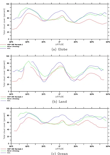
Table 2.5: Annual-mean total cloud cover (percent): the NCEP-DOE Reanalysis 2 (1979–2003 average), the Warren climatology, and the Mk3L atmosphere model (average for the final 40 years of run A-DEF).∗_{The Warren climatology only covers}

98.0% of the Earth’s surface.

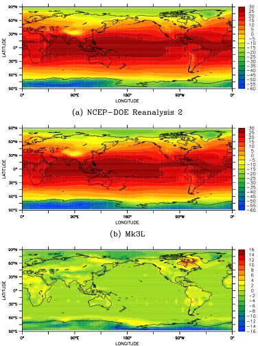
2.4.2 Cloud

Figure 2.5 shows the annual-mean cloud cover according to the NCEP-DOE Re-analysis 2, the observed climatology ofWarren et al. (1986, 1988) and Hahn et al. (1995), hereinafter referred to as the “Warren climatology”, and the Mk3L atmo-sphere model. The model can be seen to have excessive cloud cover over the tropical oceans, particularly in the western Pacific Ocean. The model also fails to reproduce the marine stratocumulus which is encountered in the north-eastern and south-eastern Pacific Ocean, and the south-south-eastern Atlantic Ocean. These clouds are often poorly simulated by climate models and yet, through reflection of sunlight, have a strong influence on the surface heat fluxes in these regions (Terray, 1998; Bretherton et al., 2004).

Figure 2.6 shows the zonal-, annual-mean cloud cover, while the global-mean cloud cover, and the means over land and over the ocean, are shown in Table 2.5. The model is generally in good agreement with the observed Warren climatology, although the excessive model cloud cover over the tropical oceans is apparent.

The simulated cloud radiative forcing is also in good agreement with observed values (Phipps, 2006).

2.4.3 Precipitation

Annual-mean precipitation is shown in Figure 2.7 for the NCEP-DOE Reanalysis 2, version 2.01 of the observed climatology ofLegates and Willmott (1990), and the Mk3L atmosphere model. While the model can be seen to reproduce the large-scale features of the global distribution of precipitation, it is only moderately successful at reproducing the positions of the monsoons.

Over the western tropical Pacific and Indian Oceans, where the simulated cloud cover is excessive (Section 2.4.2), the simulated precipitation is also excessive. Over the eastern tropical Pacific, Indian and Atlantic Oceans, however, the simulated precipitation is deficient.

NCEP-DOE Legates and Mk3L Reanalysis 2 Willmott v2.01 atmosphere

Globe 3.112 2.814 2.699

Land 2.282 -∗ _1.830

Ocean 3.441 -∗ _3.062

Table 2.6: Annual-mean precipitation (mm/day): the NCEP-DOE Reanalysis 2 (1979–2003 average), the Legates and Willmott climatology v2.01, and the Mk3L atmosphere model (average for the final 40 years of run A-DEF).∗_{No land/sea mask}

provided.

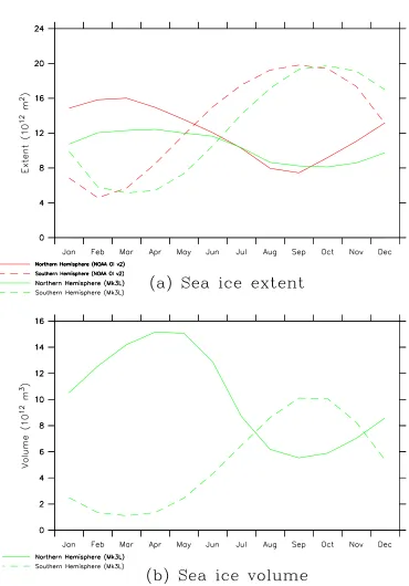
NOAA Mk3L

OI v2 atmosphere

Extent NH 12.19 10.40

(1012 m2

) SH 13.23 12.54

Volume NH - 10.17

(1012 m3

) SH - 5.19

Table 2.7: Annual-mean sea ice extent and volume, for the Northern Hemisphere (NH) and Southern Hemisphere (SH): the NOAA OI v2 analysis (1982–2003 aver-age), and the Mk3L atmosphere model (average for the final 40 years of run A-DEF). The sea ice extent is defined as the area over which the ice concentration is greater than or equal to 15%; the sea ice volume is the total volume for all gridpoints at which sea ice is present.

2.4.4 Sea ice

The simulated Northern and Southern Hemisphere sea ice extents and volumes are plotted in Figure 2.8. Sea ice extents derived from the NOAA Optimum Interpola-tion (OI) v2 sea surface temperature analysis (Reynolds et al., 2002) are also shown; this analysis combines not onlyin situ observations from ships and buoys, but also satellite observations. The standard definition of sea ice extent (e.g. Parkinson et al., 1999) is employed, which is that the sea ice extent is the area over which the ice concentration is greater than or equal to 15%.

The simulated ice extents can be seen to lag the observed values by around one month; this time lag can be attributed to the relaxation bottom boundary condition on the temperature of the mixed-layer ocean, which is employed by the stand-alone atmosphere model at high latitudes (Section 2.2.1). The simulated annual range in Southern Hemisphere ice extent is in excellent agreement with observations; in the Northern Hemisphere, the summer minimum is well reproduced by the model, but sea ice covers too small an area in winter.

Figure 2.8: Sea ice extent (1012

m2

) and volume (1012

m3

Figures 2.9 and 2.10 compare the simulated March and September ice concentra-tions, for the Northern and Southern Hemispheres respectively, with those derived from the NOAA OI v2 analysis. In the Northern Hemisphere, the deficiency in the winter sea ice extent can be seen to arise from the failure by the model to form sea ice in the Hudson Bay region. While the simulated extents in the Southern Hemi-sphere are in reasonable agreement with observations, the sea ice concentrations are much too low in both the Weddell and Ross Seas.

Figure 2.11 shows the monthly-mean sea surface temperature for the 11 sea gridpoints which constitute Hudson Bay on the Mk3L atmosphere model grid. The temperature of the mixed layer ocean does not attain the freezing point of seawater, which is taken as being -1.85◦_{C, and the model does not therefore form sea ice.}

The World Ocean Atlas 1998 sea surface temperatures, which act as the bottom boundary condition to the mixed layer ocean, do not fall below -0.92◦_{C; the failure}

of the model to form sea ice can therefore be attributed to the fact that the World Ocean Atlas 1998 sea surface temperatures are insufficiently cold.

The simulated March and September sea ice thicknesses are shown in Figure 2.12. There are no comprehensive observational datasets against which to compare the simulated thicknesses. However, Wadhams (2000), summarising the available data, indicates that ice thicknesses in the Arctic range from ∼_{1 m in the sub-polar} re-gions (such as Baffin Bay and the southern Greenland Sea) to ∼_{7–8 m along the} northern coasts of Greenland and the Canadian archipelago. In the Antarctic, un-deformed first-year ice has a mean thickness of∼_{0.6 m, while in the limited regions} where multi-year ice is encountered, such as the Weddell Sea, the mean thickness is ∼_{1.4 m. Compared to these estimates, the simulated Antarctic sea ice thicknesses} are reasonable, while the Arctic sea ice is too thin.

2.5

Ocean model evaluation

2.5.1 Water properties

The global-mean potential temperature, salinity and potential density are shown in Table 2.8, for both the World Ocean Atlas 1998 and the Mk3L ocean model. The potential temperature and potential density represent the temperature and density, respectively, that a volume of seawater would have if raised adiabatically to the surface. While the model prognoses the potential temperature, the World Ocean Atlas 1998 dataset contains in situ temperatures. These are therefore converted to potential temperature, using the multivariant polynomial method ofBryden (1973). Densities are calculated using the International Equation of State of Seawater 1980 (UNESCO, 1981), as described by Fofonoff (1985). For convenience, the quantity σθ, which represents the potential density minus 1000 kgm−3, is presented here.

Figure 2.11: The mean sea surface temperature (◦_{C) for the 11 sea gridpoints which}

constitute Hudson Bay on the Mk3L atmosphere model grid: the World Ocean Atlas 1998 (red) and the Mk3L atmosphere model (green, average for the final 40 years of run A-DEF).

World Ocean Mk3L Model

Atlas 1998 ocean discrepancy

Potential 0–800 m 9.61 10.88 +1.27

temperature 800–2350 m 2.98 3.08 +0.10

(◦C) 2350–4600 m 1.36 0.35 -1.01

Salinity 0–800 m 34.75 34.69 -0.06

(psu) 800–2350 m 34.68 34.50 -0.18

2350–4600 m 34.74 34.46 -0.28

σθ 0–800 m 26.60 26.32 -0.28

(kgm−3

) 800–2350 m 27.62 27.45 -0.17

2350–4600 m 27.81 27.64 -0.17

Table 2.8: Global-mean potential temperature (◦_{C), salinity (psu), andσ}

θ (kgm−3):

by 0.17 kgm−3

.

These biases in the properties of the deep ocean are illustrated by Figure 2.13, which shows the vertical profiles of potential temperature, salinity and σθ, and

by Figures 2.14, 2.15 and 2.16, which show the zonal-mean potential temperature, salinity andσθrespectively. Note that, in calculating the zonal means, the six inland

seas which do not have a resolved connection with the world ocean (Section 2.2.2) are excluded.

The cold, fresh and buoyant bias of the deep ocean is consistent with other comparable studies (e.g. Moore and Reason, 1993; England and Hirst, 1997; Hirst et al., 2000; Bi, 2002). The reasons for these deficiencies in the model climate are discussed in Chapter 3.

2.5.2 Circulation

Meridional overturning streamfunctions for the world ocean, and for the Atlantic and Pacific/Indian Oceans are shown in Figure 2.17. The rates of formation of North Atlantic Deep Water (NADW) and Antarctic Bottom Water (AABW) are 13.6 Sv and 9.5 Sv respectively; these are comparable with the rates obtained in other studies using a coarse-resolution version of the Bryan-Cox ocean model which incorporates Gent-McWilliams eddy diffusion (e.g. England and Hirst, 1997; Hirst et al., 2000;Bi, 2002).

Estimated values for the rate of NADW formation lie within the range 15–20 Sv (Gordon, 1986), while those for the rate of AABW formation lie within the range 5– 15 Sv (e.g. Gill, 1973;Carmack, 1977). More recent studies, based on the observed distribution of dissolved chlorofluorocarbons, estimate that the rates of NADW and AABW formation are ∼17.2 Sv (Smethie and Fine, 2001) and ∼8.1–9.4 Sv (Orsi et al., 1999) respectively. The simulated rate of AABW formation is therefore consistent with observational estimates, while the rate of NADW formation is too weak. As AABW is ∼2◦_{C colder than NADW (Orsi et al., 2001), this provides a}

possible explanation for the cold bias in the modelled deep ocean.

The annual-mean barotropic streamfunction is shown in Figure 2.18. The Ant-arctic Circumpolar Current is evident, as are the mid-latitude gyres in the Atlantic, Pacific and Indian Oceans.

The simulated rate of transport through Drake Passage is 145 Sv, which agrees well with observational estimates. Cunningham et al. (2003), using the data from six hydrographic sections conducted across Drake Passage between 1993 and 2000 as part of the World Ocean Circulation Experiment (WOCE), estimate that the rate of transport is 136.7±_{7.8 Sv.} Stammer et al. (2003), using an ocean global circulation model to assimilate WOCE data over the same period, estimate that the rate of transport through Drake Passage is 124±5 Sv. The agreement between the Mk3L ocean model and observations is particularly good when it is considered that other global ocean models simulate rates of transport through Drake Passage which range from less than 100 Sv to more than 200 Sv (Olbers et al., 2004).

condi-Figure 2.13: The global-mean potential temperature, salinity andσθ on each model

level for the World Ocean Atlas 1998 (red), and for the Mk3L ocean model (green, average for the final 100 years of run O-DEF): (a) potential temperature (◦_{C), (b)}

salinity (psu), and (c) σθ (kgm−3). The World Ocean Atlas 1998 data has been

Figure 2.14: Zonal-mean potential temperature (◦_{C) for the world ocean (excluding}

Figure 2.16: Zonal-mean σθ (kgm−3) for the world ocean (excluding inland seas):

Figure 2.18: The annual-mean barotropic streamfunction (Sv) for the Mk3L ocean model (average for the final 100 years of run O-DEF).

tion at lateral walls (e.g. Moore and Reason, 1993; Bi, 2002), and arises not only from the coarse resolution, but also from the large horizontal viscosity which is re-quired in order to resolve a viscous boundary layer at the lateral walls (Bryan et al., 1975). For the simulations analysed herein, the horizontal viscosity was set equal to 9×₁₀5 _m2_s−1_.

2.6

Flux adjustments

2.6.1 The need for flux adjustments

As discussed in Chapter 1, any change in the surface boundary conditions on either the atmosphere or ocean models, upon the coupling of the two models, will represent a potential source of drift within the coupled model. One method of minimising this drift is through the application of flux adjustments.

The oceanic meridional transports, both simulated and implied, can be derived by integrating the surface fluxes northwards from the South Pole. If the surface heat flux isFheat, then the northward transport of heatQheat is given by

Qheat(φ) =

Z 2_π 0

Z φ

−π/2

Fheata2cosφ′dλdφ′ (2.8)

where a is the radius of the Earth, andφ and λare the latitude and longitude respectively.

The surface salinity tendency dSO/dt can be converted into a surface salt flux,

through multiplication by the thickness of the upper layer of the ocean model ∆z. The northward transport of salt Qsalt is then given by

Qsalt(φ) =

Z 2_π 0

Z φ

−π/2

∆zdSO dt a

2

cosφ′dλdφ′ (2.9)

Figure 2.19 shows the northward transports of heat and salt, as simulated by the Mk3L ocean model, and as implied by the Mk3L atmosphere model surface fluxes. They can be seen to be in reasonable agreement, particularly in the case of the oceanic salt transport. This indicates that the zonal means of the flux adjustments diagnosed for the coupled model will be small.

The oceanic meridional heat transports can also be compared with observational estimates, although there are large discrepancies between the various observational datasets (Gleckler et al., 1995). Estimated values for the peak poleward transport, in both the Northern and Southern Hemispheres, range from∼_1–3.5×₁₀15_{W, with} me-dian values of∼2×1015

W in both hemispheres. The peak poleward transports simu-lated by the Mk3L atmosphere and ocean models are 1.02×₁₀15_{W and 1.18}×₁₀15_W respectively in the Southern Hemisphere, and 1.48×₁₀15 _{W and 1.14}×₁₀15 _W re-spectively in the Northern Hemisphere. These values are consistent with the ob-servational estimates, although they lie towards the lower end of the obob-servational range. The success of the atmosphere model in simulating the implied poleward heat transport in the Southern Hemisphere can be attributed to the realism of the simulated cloud radiative forcing (Gleckler et al., 1995).

2.6.2 Deriving the flux adjustments

Within the Mk3L coupled model, four fields are passed from the atmosphere model (AGCM) to the ocean model (OGCM): the surface heat flux, the surface salinity tendency, and the zonal and meridional components of the surface momentum flux. Any differences between the surface fluxes calculated by the stand-alone AGCM, and those which are required to maintain the stand-alone OGCM in its equilibrium state, will represent a potential source of drift within the coupled model. Flux adjustments are therefore applied to each of these four fields.

The derivation of the flux adjustments is straightforward. If FA is the surface

flux diagnosed from an AGCM spin-up run, andFO the surface flux diagnosed from

∆F(λ, φ, t) =FO(λ, φ, t)−FA(λ, φ, t) (2.10)

whereλ, φ, trepresent longitude, latitude and the time of year respectively. The flux adjustments therefore vary temporally, as well as spatially. Within the coupled model, ifF represents the surface flux calculated by the AGCM, then the adjusted fluxF′ _{which is passed to the OGCM is given by}

F′(λ, φ, t) =F(λ, φ, t) + ∆F(λ, φ, t) (2.11)

[Note that within Mk3L, the flux adjustments are subtracted from the AGCM surface fluxes, and therefore have the opposite sign to the values given by Equa-tion 2.10. However, EquaEqua-tion 2.10 is used to derive the values presented herein, in order to maintain the convention, followed throughout this document, that down-ward fluxes are positive.]

Four fields are also passed from the OGCM to the AGCM: the sea surface tem-perature (SST), the sea surface salinity (SSS), and the zonal and meridional compo-nents of the surface velocity. Any differences between the values of these fields, and the values which were imposed as the bottom boundary condition on the stand-alone AGCM, will also represent a potential source of drift within the coupled model. The need to apply “flux” adjustments to the components of the surface velocity is avoided through the use of climatological surface currents, diagnosed from an OGCM spin-up run, to spin spin-up the AGCM. However, “flux” adjustments are applied to the SST and SSS within the Mk3L coupled model.

The derivation of the adjustments to the SSS is straightforward. IfSobsis the SSS

which was imposed as the surface boundary condition on the stand-alone OGCM, andSO is the SSS which was simulated by the model, then the SSS adjustment ∆S

is given by

∆S(λ, φ, t) =Sobs(λ, φ, t)−SO(λ, φ, t) (2.12)

Within the coupled model, if S represents the SSS calculated by the OGCM, then the adjusted sea surface salinityS′ _{which is passed to the AGCM is given by}

S′_{(λ, φ, t) =S(λ, φ, t) + ∆S(λ, φ, t) (2.13)}

The derivation of the adjustments to the SST is more complex. If TAis the SST

which was imposed as the surface boundary condition on the stand-alone AGCM, and TO is the SST simulated by the stand-alone OGCM, then the SST adjustment

∆T is given by

∆T(λ, φ, t) =TA(λ, φ, t)−TO(λ, φ, t) (2.14)

However, the stand-alone OGCM uses a mixed-layer ocean to calculate the SST at high latitudes. If Tobs is the SST which was imposed as the surface boundary

condition on the stand-alone AGCM, and ∆Tmlo is the temperature of the

mixed-layer ocean (expressed as an anomaly, relative to the value ofTobs), thenTAis given

TA(λ, φ, t) =Tobs(λ, φ, t) + ∆Tmlo(λ, φ, t) (2.15)

Substituting this value forTA into Equation 2.14, the SST adjustment is given

by

∆T(λ, φ, t) =Tobs(λ, φ, t) + ∆Tmlo(λ, φ, t)−TO(λ, φ, t) (2.16)

The SST adjustments are applied on the atmosphere model grid. Prior to using Equation 2.16 to calculate the SST adjustments, it is therefore necessary to interpo-late the ocean model SSTTO onto the atmosphere model grid, in exactly the same

fashion as takes place within the model.

2.6.3 Fields passed to the ocean model

Zonal means

Figure 2.20 shows the zonal-mean surface fluxes diagnosed from Mk3L atmosphere and ocean model runs A-DEF and O-DEF, and the zonal-mean flux adjustments which are diagnosed for use in the coupled model. As anticipated from the agreement between the simulated and implied oceanic meridional heat and salt transports, the zonal-mean surface heat flux and surface salinity tendency adjustments are small, not exceeding 34.1 Wm−2

and 1.55 psu/year in magnitude.

The largest zonal-mean heat flux adjustments arise at the equator, where the atmosphere model simulates a larger net downward heat flux than the ocean model; at mid-latitudes in both hemispheres, where the atmosphere model simulates a net downward heat flux, while the ocean model simulates a net upward heat flux; and beneath sea ice, where the atmosphere model simulates a larger net upward heat flux than the ocean model.

The zonal-mean surface salinity tendencies agree well, with both the atmosphere and ocean model simulating positive salinity tendencies (corresponding to an excess of evaporation over precipitation) in the sub-tropics, and negative salinity tendencies elsewhere. Only in the Arctic Ocean, where the high spatial variability of the World Ocean Atlas 1998 sea surface tendencies gives rise to high spatial variability in the surface salinity tendency simulated by the ocean model, does the zonal-mean flux adjustment exceed 1 psu/year.

The zonal-mean zonal momentum flux simulated by the atmosphere model is in reasonable agreement with the NCEP-DOE Reanalysis 2, although the maxima in both hemispheres are slightly too weak, and too close to the equator. As a result, the zonal-mean flux adjustment is small, except for peaks of∼_{0.10 Nm}−2_at∼₆₀◦_{S, and} ∼0.09 Nm−2

at ∼60◦_{N. The simulated zonal-mean meridional momentum flux is in}

good agreement with the NCEP-DOE Reanalysis 2, and as a result the zonal-mean flux adjustment does not exceed 0.033 Nm−2

in magnitude.

Spatial variability

surface salinity tendency, high spatial variability is encountered, with large contrasts occurring between the flux adjustments applied at adjacent gridpoints.

The large-scale spatial structure of the heat flux adjustments (Figure 2.21c) is dominated by variations in the zonal direction, rather than in the meridional direc-tion. Positive adjustments (i.e. heat being added to the ocean) are required along the western boundaries of the ocean basins, while negative adjustments (i.e. heat being removed from the ocean) are required along the eastern boundaries. The pos-itive heat flux adjustments can be attributed to the failure of the ocean model to adequately resolve the western boundary currents (Section 2.5.2); as a result of this failure to advect heat polewards from the tropics, this heat must instead be sup-plied in the form of flux adjustments. The negative heat flux adjustments can be attributed to the failure of the atmosphere model to simulate the marine stratocu-mulus which occurs along the eastern boundaries of the ocean basins (Section 2.4.2); the surface heat flux is therefore excessive, and must be adjusted accordingly.

Relatively large heat flux adjustments also occur within the Southern Ocean. These tend to take the form of dipoles, with adjacent positive and negative flux adjustments; it is therefore hypothesised that they arise from a failure by the ocean model to correctly simulate the finer-scale structure of the Antarctic Circumpolar Current.

The surface salinity tendency adjustments (Figure 2.22c) are generally small, and exhibit no large-scale spatial structure. Large adjustments do occur, however, in the Arctic Ocean, and in the vicinity of the Amazon Delta. The large salinity tendency adjustments in the Arctic Ocean can be attributed to the high spatial variability in the surface salinity tendency simulated by the ocean model. The large adjustments in the vicinity of the Amazon Delta can be attributed to the large mismatch between the surface freshwater fluxes simulated by the stand-alone atmosphere and ocean models.

The relatively large adjustments to the zonal momentum flux at ∼₆₀◦_{S and} ∼₆₀◦_{N are apparent (Figure 2.23c). Particularly large adjustments are applied in} the North Atlantic, where the maximum in the atmosphere model momentum flux lies further south than in the NCEP-DOE Reanalysis 2, and across the Southern Ocean. The adjustments to the meridional momentum flux are small (Figure 2.23d).

Temporal variability

In addition to the spatial variability exhibited by the flux adjustments, they also exhibit temporal variability in the form of an annual cycle. Figure 2.24 shows the root-mean-square amplitude of the annual cycle exhibited by the adjustments to each of the four surface fluxes. The amplitudes can be as large as 229 Wm−2

in the case of the surface heat flux adjustments, 21.4 psu/year in the case of the surface salinity tendency adjustments, and 0.104 Nm−2

in the case of the momentum flux adjustments.

While the annual-mean flux adjustments can be large in magnitude, the monthly-mean adjustments, which represent the values which would actually be applied within the coupled model, are even larger. Table 2.9 shows some statistics for the adjustments diagnosed for each of the four surface fluxes. The surface heat flux adjustment can be as large in magnitude as 443.68 Wm−2

Figure 2.21: The annual-mean surface heat flux (Wm−2

Figure 2.23: The annual-mean surface momentum flux (Nm−2

Figure 2.24: The root-mean-square amplitude of the annual cycle in the flux ad-justments: (a) the surface heat flux (Wm−2

), (b) the surface salinity tendency (psu/year), and (c), (d) the zonal and meridional components, respectively, of the surface momentum flux (Nm−2

Field Units Annual means Monthly means

Mean RMS Min Max Min Max

Heat flux Wm−2

+0.20 45.21 -208.10 +247.90 -386.55 +443.68

Salinity psu/ -0.00 1.69 -13.08 +27.83 -43.14 +51.55

tendency year

τx Nm−2 +0.012 0.041 -0.110 +0.186 -0.187 +0.333

τy Nm−2 +0.001 0.019 -0.100 +0.076 -0.200 +0.192

Table 2.9: The flux adjustments diagnosed from the final 40 years of Mk3L atmo-sphere model run A-DEF, and the final 100 years of Mk3L ocean model run O-DEF, for the surface heat flux, the surface salinity tendency, and the zonal and meridional components of the surface momentum flux (τx,τy). For each field, the global-mean,

root-mean-square, minimum and maximum values of the annual-mean flux adjust-ments are given, as are the minimum and maximum values of the monthly-mean flux adjustments.

tendency adjustment can be as large in magnitude as 51.55 psu/year, equivalent to a freshwater flux of∼_{37 m/year.}

Such adjustments are comparable to, or even larger in magnitude than, the fluxes which are being simulated. The surface heat flux adjustment, for example, can be larger in magnitude than the incoming flux of solar radiation, which provides the only physical energy input to the climate system. Even under clear skies and at the equator, the daily-mean insolation cannot exceed∼_{434 Wm}−2

(representing the value of the solar constant, divided byπ). It is therefore the case at some locations, particularly at high latitudes, that the flux adjustments will represent the largest component of the surface fluxes which are applied to the ocean.

2.6.4 Fields passed to the atmosphere model

Figures 2.25 and 2.26 show the annual-mean adjustments to the sea surface tem-peratures and salinities. Unlike the adjustments applied to the surface fluxes, the adjustments to the sea surface temperature (SST) and sea surface salinity (SSS) are relatively small in magnitude. This is particularly true in the case of the annual-mean SSS adjustments, which do not exceed 0.75 psu in magnitude.

The adjustments to the SST reflect the deficiencies in the climate of the stand-alone ocean model. The adjustments are generally positive at low latitudes and negative at high latitudes, representing the tendency of coarse-resolution ocean gen-eral circulation models to simulate tropical SSTs that are too cold, and high-latitude SSTs that are too warm (e.g. Gordon and O’Farrell, 1997).

Figure 2.25: The annual-mean sea surface temperature (◦_{C): (a) the Mk3L}

Figure 2.26: The annual-mean sea surface salinity adjustment (psu), diagnosed from the final 100 years of Mk3L ocean model run O-DEF.

Field Units Annual means Monthly means

Mean RMS Min Max Min Max

SST ◦_{C +0.003 0.566 -3.855 +2.362 -7.506 +5.468} SSS psu -0.000 0.082 -0.752 +0.579 -3.388 +2.990