A Framework of Filtering, Clustering and Dynamic Layout Graphs
for Visualization
Xiaodi Huang
1, Peter Eades
2, Wei Lai
31Department of Mathematics and Computing, the University of Southern Queensland, Toowoomba, Australia 2National ICT Australia limited, Sydney
3Faulty of Information Technology and Communication, Swinburne University of Technology, Melbourne
[email protected]; [email protected]; [email protected]
Abstract
Many classical graph visualization algorithms have already been developed over the past decades. However, these algorithms face difficulties in practice, such as the overlapping node problem, large graph layout and dynamic graph layout. In order to solve these problems, this paper aims to systematically address algorithmic issues related to a novel framework that describes the process of graph visualization applications. First of all, a framework for graph visualization is described. As the important parts of this framework, we then develop two effective algorithms for filtering and clustering large graphs for the layouts. As for the dynamic graph layout, a new approach to removing overlapping nodes called force-transfer algorithm is developed. The framework has been implemented in a prototype called PGA to demonstrate the performance of the proposed algorithms. Finally, a case study is provided.
Keywords: information visualization, graph visualization,
graph drawing, framework, filtering, clustering.
1
Introduction
Many models have already been presented in information visualization (Shneiderman 1996, Haber et al 1990, Card et al 1999, Eades et al 2000, Chi 2000, Kreuseler et al 2002, Cristina et al 2003). These models focus on different aspects of visualization such as visualization process, design, and guideline. In the following, we review such three typical models.
Shneiderman (1996) pointed out that the basic principle of visual design can be summarized as the visual information seeking mantra: overview first, zoom and
filter, then details-on-demand. Based on this mantra, the
taxonomy for the design of information visualization systems is proposed to make connections between visualization data types and tasks. Types of such data are identified as 1-, 2-, or 3-dimensional, temporal, multi-dimensional, tree, and network. The tasks that users can perform on these data include overview, zoom, filter,
details-on-demand, relate, history, and extract. Based
users’ perspective, this taxonomy classifies seven tasks associated with various types of data. Information
Copyright ©2005, Australian Computer Society, Inc. This paper appeared at the 28th Australasian Computer Science Conference, The University of Newcastle, Australia. Conferences in Research and Practice in Information Technology, Vol. 38. V. Estivill-Castro, Ed. Reproduction for academic, not-for profit purposes permitted provided this text is included.
Visualization Data State Reference Model (Chi 2000) divides a visualization data pipeline into four distinct stages, namely value, analyticalabstraction, visualization
abstraction, and view. The transformation between those
stages requires one of data transformation operators including data transformation, visualization
transformation, or visual mapping transformation. This
model associates the crucial visualization operations with the visualization pipeline.
In the area of graph visualization, P. Eades and Huang (Eades et al 2000) initiated a layered architecture for presenting clustered graphs. This architecture encompasses graph, clustering, abridgement and picture
layers. Users can directly manipulate data in these layers by a set of operations provided. After gathering a graph data, a group of related nodes in the graph are clustered into a hierarchical clustering node superimposed. The architecture supports abridgments of clustered graphs, andlogical views of parts of the clustered graph. Users can focus on special areas of the graph by changing the
abridgment. These changes are immediately reflected in
the picture of the abridgment. It is clear that this
architecture is particularly proposed for clustered graphs. The above models or architecture are user-oriented, and data (or graph) oriented. Indeed, these models present a picture of how data (or graph) is transformed and with what kinds of tasks users are confronted at each stage of this transformation. They do not, however, systematically address issues associated with graph applications in realistic application settings. From a practical perspective, we need to concentrate on questions such as what the steps for applying a large number of existing layout algorithms (Battista et al 1999) into real graphical applications are.
In this paper, we propose a framework for practical graph visualization with the following purposes:
• To establish a conceptual framework within which graph visualization systems can be classified and compared.
• To describe a pipeline of applied graph visualization systems.
• To develop a number of algorithms associated with such a framework.
• To advance the description, comprehensiveness and exchange of ideas in graph visualization.
algorithm for adjusting layouts is presented in Section 5. The implementation of this framework called PGA is briefly described in Section 6, followed by the conclusion in Section 7.
2
A New Framework for Graph Visualization
In this section, we will identify the characteristics of graph visualization applications and then present a framework.
2.1 Characteristics of Graph Visualization
Applications
There are many graph visualization applications, ranging from Web sites to gene visualization. The characteristics of graph visualization applications are thus enormous. However, our main concern here is to find the characteristics of graphs that are highly related to the techniques for graph visualization.
2.1.1 Attributed Graphs
As we know, a graph is employed to model relational objects, where the nodes denote objects, and the edges represent the relations between these objects. In traditional graph visualization, a node is mapped into an abstract point in a Cartesian plane, occupying almost no screen space. An edge is a line connected to two nodes in the graph. The reality is, however, that every object has a set of properties, and every edge is also associated with a set of attributes. In order to incorporate more semantic information about the properties of both objects and relations, attributed graphs (AGs) or attributed relational
graph (ARG) were employed in many areas (Fu et al
1979, Bunke 1993, Bunke et al 1997, Lourens 1998, Walischewski 1997). Therefore, the problem of how to visualize attributed graphs should receive much more attention in the field of graph visualization (Huang 2001). A labeled graph, a special case of attribute graphs, is another kind of widely used graphs, which has labels attached to each node or edge.
2.1.2 Large Graphs
In reality, graph visualization applications typically deal with very large graphs. A good example of this is telephone billing records. The nodes of this “call graph” is telephone numbres, and the edges are calls made from one number from another. A one day call graph has 53,767,087 nodes and 170 million edges (Abello et al 1999). The Hollywood collaboration graph is the second example where the nodes are 225,000 actors, and an edges connects any two actors who have appeared in a feature film together. If we regard the World Wide Web as a graph, this Web graph has 4.3 billion ( according to the 27 Feb, 2004 Google homepage) pages as the nodes and hyperlinks from one page to another as the edges. Various techniques have already been developed to tackle the problem of large graph visualization. Broadly categorizing large graphical data as distortion-oriented
and non distortion-oriented presentations, Leung (1994) provided a simple taxonomy of techniques for such presentations. These techniques include encoding, spatial transformation (geometric), data suppressing (abstraction and threshold), zooming, windowing, and paging and clipping. As two important techniques for data suppressing, filtering and clustering reduce the size of a graph by removing pars of information.
2.1.3 Dynamic Graphs
Graph drawing involves a repeat redrawing resulting from frequent changes of the graphs. Although graph layout is traditionally viewed as static, dynamic and interactive graphs have many applications. As an example, an interactive graph system should provide flexible facilities such as insertion or deletion of nodes, and open or close of subgraphs, which cause regular adjustments of the graph layout.
2.2 A Framework for Graph Visualization
Along with the analysis of characteristics of graphical visualization applications, we propose a framework for graph visualization, as illustrated in Fig. 1.
Graph visualization can alternatively be viewed as adjustable mappings from relational data to visual forms, and then to users. The information on the left side of Fig.1 is to be graphically visualized while users on the right can directly manipulate the visualized information. The right-direction arrows andthe arrow between views
and users indicate the possible adjustments of these
transformations by the users. In this pipeline, the original abstract relational data undergoes several processing stages in order to achieve a graphical view.
Relational data: The data to be visualized, which can be
broadly classified into two categories: online and offline.
Graph representation: The structure of relational
information can be modelled as a set of entities and their relationships. A graph G = (V, E) is commonly used to represent it, where V denotes the entities, and E the relationships between the entities.
Filtering: There are two meanings of filtering. Filtering
removes noise nodes and their associated edges in a graph. In application settings, the transformation from relational data into a graph is automatically extracted by a computer programme. This may lead to producing some “noise” nodes. For this reason, manipulating the raw graph is required in order to remove those “noise” data. On the other hand, Filtering can suppress unimportant nodes and their related edges to highlight those important nodes by using an adjustable threshold to control appearances of the nodes. Clustering: If a graph is too large to fit on the screen, groups of related nodes are “clustered" into super-nodes. Users see a “summary" of the graph, namely the super-nodes and super-edges between the nodes. Some clusters may be shown in more detail than others. The process of clustering involves
Fig. 1. A framework for graph visualization pipeline Relational Data
Graph
discovering groups in the data In the case of graph visualization, clustering means finding a setof relatively highly connected nodes and their associated edges in a graph, and then using a special type of node called a meta-node or super-node to represent them. In other words, the clustering techniques make it possible to represent a graph by displaying fewer elements, allowing users to control the level of detail by “opening” and “closing” meta-nodes. The clustering approach has been taken by a number of graph drawing researchers (Eades et al 1996, Dongen 2000, Fowlkes et al 2001).
Layout: Apply an algorithm to layout a given graph.
View: With a layout, users may interact with the graph,
changing the view in order to gain insight into the data. This feature requires that a system should easily adapt to the users’ needs and quickly change the way in which a graph is presented. In addition to navigating it, the users are able to explore a graph. Moreover, the users should enable to interactively apply criteria that may result in different sets of clusters within the data.
In the above framework, the filtering and clustering
stages are optional in the case of the small number of nodes and edges in a graph. The filtering stage can also be omitted in some applications. The View stage is highly related to the layout stage in that every view results from re-layout of the graph.
Motivated by applying existing algorithms to applications, we proposed the framework derived from the general requirements of real graphical applications. It is this feature that mainly distinguishes it from other models described previously.
In the following sections, we will focus on the development of algorithms for filtering, clustering, and dynamic view used in the above framework.
It is assumed that we have a graph G= (V, E), where V= {1, 2, … , |V|} is the set of nodes, and E⊆ ×V Vis the set of edges.
3
Filtering Graphs
Graph filtering refers to selecting particular nodes and edges from a graph. It is a way of reducing the graph size by moving “noise” nodes, and of highlighting important nodes.
Huang et al. (1998) applied several rules to filter a real Web graph into a simplified tree for a nice layout. The rules include the graph structure-based rule, Web context structure-based rule, information-based rule, document structure-based rule, and link number-based rule. The use of these rules ensures that the converted graph is a tree, and simplifies the original Web graph by removing some particular nodes and their associated edges. It is obvious that huang’s rules are concerned with both the structure and content of a Web graph.
Simple filtering techniques based on node attributes are also reported in Henry’s thesis (Henry 1992).
The above approaches have some limitations. The approach of Huang et al., for instance, is confined to a
specific type of graph, namely Web graphs, and does not suffice to handle other types of graphs. Therefore, it is necessary to develop a more sophisticated technique for filtering general graphs.
The approaches to filtering graphs can be roughly classified into structure and content-oriented. The structure-based approach utilizes the linkages of a graph while the content-based one uses the semantic contents of what the nodes represent. Our approach is a structure-based one and thus has the advantage of being applicable to any type of a graph.
As mentioned before, graph filtering involves in the selection of nodes and edges from a graph according to whether the values of their attributes fall within a specified range. The purpose of the use of a graph is to visually represent complex relationships between objects or entities in order to reduce the cognitive load. Various nodes and edges in a graph, however, play different roles in revealing such relationships. Some are prominent while others are trivial. Prominent nodes are those that are extensively involved in the relationships with other nodes. This involvement makes them more visible to the others. For this reason, it is necessary to develop a method to clearly identify the “important” nodes in a graph. A function is needed to measure the importance roles of nodes with respect to the depiction of relationships. Fundamental to our approach is the notion
of Node Importance Score, which is defined as follows:
Definition Node Importance Score (NIS): A real number indicating the degree of the importance role in which a node plays within a graph, or of the involvement of a node in other relationships. Let G = (V, E) be an undirected and connected graph, and Rbe a function that assigns a real value ranging from 0 to 1 to every node i in
G. That is,R:V →[0, 1]. The Node Importance Score of node u denoted by R(i) (0≤R(i)≤1) is used to rank nodes.
With this definition, it follows that we need to develop a method for the calculation of a NIS.
The following algorithm is proposed on the basis of the fact that the NIS of a node is affected by the NISs of nodes to which it connects and by itself.
3.1 Computing NIS of Each Node
The importance of nodes that are proximate to the node under study should contribute to that of this node. Based on this fact, the NIS of a node should be proportional to the sum of the NIS of the nodes to which it is directly connected. Therefore we have:
∑
=
= n
j j ij
i a r
r
1
λ
On the other hand, some status importance of nodes does not completely depend on their connection to others. Each student in a class, for example, has some popularity that depends on his or her external status characteristics. In a word, each individual node has its own status characteristics, which are independent of other nodes. Overall, the measure of the importance of a node is determined by both external and internal factors. The above equation can thus be modified as:
i n
j j ij
i ar e
λ
r =
∑
+=1
where ei is the internal importance score of node i. The parameterλ reflects the relative importance of exogenous versus endogenous factors in the determination of NIS. These n equations for all nodes in a graph can be rewritten in a matrix form. Let r be a vector of NIS,
i.e. '
) (r1,r2,L,rn =
r , e a vector of the internal importance
of nodes, i.e. '
) (e1,e2,L,en =
e , and A an adjacent matrix. An equation with a combination of both external and internal factors is then given by:
e r r= T +
A
λ
This equation has a matrix solution:
e I
r=( −λ T)−1
A
where I is an identity matrix with d dimensions, and eis a vector with n components.
We normalize r to the norm of 1, i.e.
1 |
| 1
2=
=
∑
=
n i
i
r r
The eigenvector importance of a node i is finally attained:
i
r i
R( ) =
That is, the components of vector r are the corresponding
NIS of nodes in a graph. High rank importance scores imply that nodes are connected either by a few other nodes that have high rank scores, or by many others with low to moderate rank scores.
The running time for computing NIS is O(n ^2.376) (Coppersmith 1990).
This idea of eigenvector centrality was initiated by (Katz 1953) and further developed by (Hubbell 1965) and many others, finally culminated with (Bonacich 1972) who defined centrality as the principal eigenvector of an adjacency matrix.
Up to this point, we already know to how to calculate the
NIS of a node in a graph. However, we cannot directly remove those nodes with relatively lower NISs. The underlying requirement for filtering is that a filtered graph is still connected, which means that the main relations of what the graph reveals are well preserved. The removal of some nodes disconnects a graph. Also, their removals make some nodes unreachable from some others. These nodes are referred to as cutpoints. Similarly, edges are bridges if their removals result in disconnected subgraphs. Therefore the second main step of filtering a graph is given in the following section.
3.2 Filtering Nodes and Edges
The nodes in the graph are ranked according to their
NISs, and those nodes as well as their associated edges are then removed which are not cutpoints and bridges, and whose NISs are less than the threshold. Formally, the set of filtered nodes is
)}) )
( )
{(
}, ) ( ) ( |
({
(G u v, V u | u v,
t v R G K v V v v F
λ ∉ ∧ ∈
< ∧ ∉ ∧ ∈ =
where k(G) denotes the set of cutpoints in a graph
G,λ(G) denotes the bridge set including all bridges, and
R(v) is the NIS of node v .
This model for filtering graphs is called global filtering, while another model is known as fisheye filtering. Both models are based on thresholds. Global filtering, however, permanently removes relatively unimportant nodes and their associated edges, measured by their NISs. In other words, the appearance of a particular node is primarily determined by its NIS. Within the fisheye
filtering model, whether a node is visible or not is
conditional on both the NIS of this node and its distance from the current focus node.
3.3 An Experimental Example
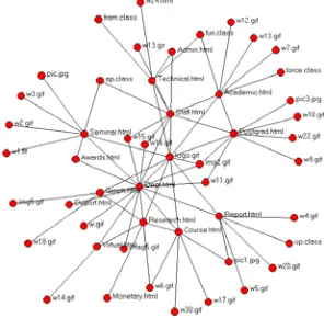
An example of a Web graph with 50 nodes is shown in Fig 2(a), while Fig 2(b) illustrates the filtered graph with 27 nodes. It is obvious that the nodes at marginal areas have been removed. This conforms to the concept of NIS
defined before.
(a) A graph with 50 nodes, and their Node Importance
Scores ranging 2.874%~ 64.998 %
(b) A filtered graph with 27 nodes, and their Node
[image:4.595.347.495.421.566.2]Importance Scores ranging: 7.474%~64.998 %
[image:4.595.372.471.601.722.2]4
Clustering Graphs
Apart from filtering, clustering graphs serves as an efficient alternative method of drawing large graphs. Clustering a graph means that relatively highly connected nodes and their associated edges are grouped to form a subgraph, represented by one abstract node. In this way, a coarse, clustered graph is obtained by replacement of all such subgraphs. A clustered graph can greatly reduce visual complexity. Moreover, a hierarchically clustered graph can produce superimposed structures over the original graph through a recursive clustering process. In the field of graph visualization, a node structural metric is widely utilized in many different forms. One simple example is the degree of a node, i.e., the number of edges connected to the node. A metric more specific to trees, called the Strahler metric, is applied to tree graphs, in which nodes with the highest Strahler metric values generate a skeleton or backbone, which is then emphasized (Delest et al 1998, Herman et al 1999). Using the distance metric, R.A. Botafogo et al. (1992) constructed a distance matrix that has as its entries the distances of every node to every other node, to identify hierarchies in an organization.
In what follows, we present a new approach to clustering a graph. The key idea behind this approach is to use an abstract node to express a set of the most linked nodes in a graph. This is achieved by initially grouping linking nodes from a node linkage matrix constructed on the basis of a novel node link metric. Such each group potentially represents a set of highly connected nodes in the graph. These groups are then individually replaced with abstract nodes to form a higher abstraction level of the graph with a reduced dimension.
4.1 Linkage Matrix
In order to find those subgraphs with high connectivity in a given graph, we need a measure to quantify the linkage degree of a graph. Starting with a simple case of two nodes, we discuss this linkage between them. A node structural metric is thus proposed to measure such a link between two nodes, making use of the number of shared edges and how many links they have. The link degree between two nodes is partly determined by the number of edges between them. In particular, the greater the number of the edges the two nodes share, the more links they are. At the same time, the greater the number of edges they do not share, the less link they are. For this reason, a linkage measure function is needed. The measures that occur most in the literature are the dot product, Euclidean distance and the Jaccard Coefficient (Everitt 1993). Among them, Jaccard Coefficient can be used to measure the degree of overlap. We therefore calculate the degree of the connection between two nodes l and k as
1 ( , ) 1
deg( ) deg( ) 1
Link l k
l k
= −
+ −
where the degree of node l, namely deg( ) | { | ( , )l = i l i ∈ ∧ ∈E i V} |, is the number of nodes that are directly connected to it.
In general, it is possible for two non-neighbour nodes in a graph to have more than one or no paths between them. We aim to maximize the linkage degree between the two nodes. Obviously, the longer the path between two nodes is, the less the linkage value they have. The maximum linkage degree of two nodes can consequently be considered as finding the shortest path with respect to the minimum cost in the graph where the cost of every edge is 1.
For the above reason, the need for finding the shortest paths between all pairs of nodes in a graph arises. More precisely, the shortest paths between two non-neighbour nodes, defined as a path with the fewest edges, are initially found by the well-known Dijkstra or Floyd’s algorithm. The products of sequentially multiplying linkage values of all node pairs in such paths are then calculated. Finally, the maximum value among those products is chosen as the degree of linkage between the two nodes. Formally, it is assumed that one of the shortest paths between nodes vi and vj is along a sequence of node pairs (vi, vk), (vk, vl) ,…, (vm, vj). The linkage value l (vi,
vj) maximizes all the values of Link(vi, vj) over all the possible shortest path sets, denoted by a union set P′,
between nodes vi and vi. An equation is accordingly arrived at:
'
( , )
( , ) max{ ( , )}
P l k P
l i j Link l k
∈
=
∏
where P is a set of pairs of nodes in the shortest path between nodes i and j, namelyP={(l,m),L,(r,k)}. Such several possible shortest paths consist of a set '
P.
Combining of the above two equations, we can construct the node linkage matrix of a graph G. Each entry of this matrix is computed by the above equation which tells the extent to which two nodes are linked. The node linkage matrix is thus derived:
| | | | [ ( , )]V V
L= l i j ×
This matrix provides a basis for clustering the corresponding graph.
4.2 Seed Node
With the linkage matrix L of a graph, we attempt to find highly connected subgraphs. Such subgraphs can be found using the seed nodes as their first member nodes. A number of different schemes have been developed for selecting an initial set of seed nodes as the centroids of clusters. A commonly used scheme selects the seeds at random. A clustering solution is then computed using each one of these sets. The quality of such clusters is evaluated by computing the similarity of each node to the centroid vector of the cluster that it belongs to. The best solution is the one that maximizes the sum of these similarities over the entire set of nodes.
Starting with arbitrary random centroids is, however, a relatively poor solution. An efficient method is presented here to determine the number of clusters and then to choose the initial centroids of the clusters.
more connectivities to other nodes, should form a local “community” together with the nodes around it.
The proposed algorithm detects as the seed nodes the nodes whose degrees are greater than the average degree of a graph G. These nodes potentially act as the initial members of different clusters later. In some cases, two or more seed nodes, however, are densely connected and they are not far away in the graph. This suggests they should stay within one cluster. Such two or more seed
nodes will be combined into one seed node, if they share
the nodes of their k-nearest neighbour node sets, denoted by k-NN, and if the number of the shared nodes is no less than half a degree of one of them. Each remaining member of the reduced seed node set acts as the initial member of each cluster.
The seek nodes are chosen against the following two
criteria:
• Their degrees are above the average degree of the graph
( ) { | deg( ) deg( ), }
N G = i i > G i∈V
• If two nodes satisfying the above criterion are not far away in the graph, then remove one of them.
G N i, j /2, j deg | j k_NN i
k_NN | j G
N'( )={ ()∩ ( ) ≥ ( ) ∈ ( )}
where k_NN(i) is the k-nearest neighbour set of node i. The nodes in a setN G( )=N G( )−N G'( )will be seed
nodes.
4.3
k
-means Algorithm
With a set of seed nodes, we can apply the k-means algorithm to the linkage matrix so as to group highly linked nodes into subgraphs in a graph. The algorithm consists of a simple re-estimation procedure as follows. First, the nodes in the seed nodes set N(G) are individually assigned to the |N(G)| cluster sets as their initial memberships. The centroid is then computed for each clustering set. These two steps are alternated until a stopping criterion is met, i.e. when there is no further change in the assignment of the nodes. Recursively applying the k-means algorithm to the matrix produces the multiple abstraction level of clustered graphs.
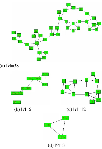
We report an experimental example to show the results in Fig. 3. To deal with the problem of large graph layouts,
filtering and clustering have the identical purposes of
reducing the number of nodes and edges within a layout. However, filtering achieves this by suppressing part of a graph, removing less important information. On the contrary, clustering forms higher-level summaries by grouping nodes and edges, hiding parts of information.
5
Changing Views
In practical graph visualization applications, the nodes in a graph represent objects or entities, which have distinct labels as their identifiers. These labels in a drawing can be presented in the form of texts, digitals, or images that should be drawn not as abstract points with almost no size that most drawing algorithms assume, but rather as rectangles large enough to display the labels. For example, UML diagrams in CASE tools are labeled
(a)|V|=38
(b) |V|=6 (c) |V|=12
[image:6.595.306.515.53.359.2](d) |V|=3
Fig.3. Graphs and their clustered graphs
graphs, a special attributed graph as we mentioned before. The problem of node overlapping may occur when applying traditional graph layout algorithms to such labeled graphs, most of which do not take into account the node size. This results in destroying the layout aesthetics—the main purpose of the layout algorithm. The need for removing overlapping nodes thus arises. Furthermore, in a dynamic environment where a graph can often be modified such as enlarge/shrink subgraphs and add /delete nodes, also at the view stage of the proposed framework, users need to interactive with a layout, the layout of the graph should thus be adjusted to cater for these changes. When eliminating overlapping nodes, it is desirable that adjustment of the original layout should be kept to a minimum.
2000). The Force-based Algorithm includes Cluster Busting in an anchored graph drawing and the Force-Scan algorithm (FSA). The procedure of Cluster Busting is iterative in that the nodes in a graph are iteratively relocated in accordance with measurable criteria. These criteria are introduced to improve the distribution of the nodes (cluster busting) and to minimize differences between the original layout and adjusted layout (anchored graph drawing). Also, these algorithms have to run several iterations to achieve a better-adjusted layout. Preserving the mental map of an original graph, FSA produces a compact layout compared with the Uniform Scaling. A variant of FSA (Lai 1993) allows an additional pull force between two nodes to make a graph layout as compact as possible. Other related work includes the SHriMp Algorithm (Story et al 1995), where the nodes in a graph uniformly give up screen space to allow a node of interest to grow. These nodes are appropriately scaled to fit inside the screen.
We present an adjusted graph layout Algorithm called Force-Transfer Algorithm (FTA).
The main idea of FTA is to apply a ‘force’ f vu to one of
two overlapping nodes v and u so that fvu pushes u away
from v. For all the overlapping nodes in a graph, applying forces is carried out one by one within two scans: one left-to-right horizontal scan, and another top-to-bottom vertical scan. As a result, some nodes are moved in either horizontal or vertical directions to avoid overlaps. This scheme raises three issues to be addressed: how great the force should be, in which way an applied force is transferred to other nodes, and where to start with the first force. The answers that follow to these questions make a distinction between FTA and the widely used FSA. First, a minimum force is chosen to separate two overlapping nodes so that the local optimisation of an adjustment is achieved. Second, the force is restrictedly transferred to a dynamic subgraph that is a group of nodes overlapping each other. It is possible that a node does not overlap with any node in the subgraph, but does with at least one of them after an adjustment. The nodes in the subgraph are therefore updated iteratively during the scan. The process of the adjustment will continue until such subgraphs including overlapping nodes no longer exist in the final layout. It should be noted that the node with the initial applied force called the seed node in FTA can be any node in a graph.
The algorithm is described as follows:
Input: A graph G layout
Output: An adjusted layout without overlapping nodes
Sort all the nodes according to the values of their x1i
(the left-upper corner) coordinates Start scan from the leftmost node Right horizontal scan
Down vertical scan
In the following we take the right horizontal scan as an example to explain its procedure.
• Compute overlap distances between two nodes i and j
Fig. 4. Overlap calculation
| |
2 / )
( i j i j
ij w w x x
dx = + − −
| |
2 / )
( i j i j
ij h h y y
dy = + − −
where wi, hi, wj and wj denote the widths and heights of
nodes i and j, respectively.
• Find all left (or down) nodes recursively overlapping with a particular node j
LNN j( )={( , ) |i j i< ∧j dxij > ∨0 dyij >0}
For instance, while overlapping with node a, node b
overlaps with node c, then we have LNN (b) = {(a, b), (b, c)}.
• Calculate an orthogonal force
<
=
otherwise dy dx if dx
fx ij ij ij
ij
0 and
≥
=
otherwise dy dx if dy
fy ij ij ij
ij
0
That is, we use only the minimum one of two orthogonal overlapping distances.
• Aggregated distances of each node
A node will receive all applied forces on the nodes at its left side if they are overlapping each other. Thus we have
∑
∈= ) ( ) , (ij LNNk
x ij x
k f
d
where k = 2,…, |V|. • Reposition each node.
x k k
k x d
x = + , yk = yk
From left to right, the overlapping nodes are moved to the right one by one, including those newly overlapping nodes due to this adjustment.
Two examples are given in Fig 5. More examples and comparison with FSA were reported in (Huang et al 2003).
6
A Prototype of the Framework and Example
Employing the object oriented design, we develop a prototype for the proposed framework called PGA so as to demonstrate the performance of our algorithms and approaches.
The user interface of PGA is shown in Fig 6. The architecture of PGA is composed basically of several modules: input module, filter module, cluster model,
layout Module, and view module.
There modules roughly match the graph visualization framework shown in Fig. 1. The modules can be seamlessly assembled into a graph visualization application in which each module corresponds to one stage of processing in a pipeline of graph data flow in the proposed framework.It is also possible, of course, to use
dyij
dxij (xi , yi)
(xj , yj)
i
the modules independently such as the filtering module,
the clustering module, and the layout module.
(a) An overlapping graph layout
(b) Layout adjusted by the force-transfer algorithm
(c) An overlapping graph layout
[image:8.595.60.277.44.690.2](d) Layout adjusted by the force-transfer algorithm Fig. 5. Overlapping graph layouts and their adjusted
[image:8.595.96.254.81.168.2]layouts
Fig. 6. The interface of the framework PGA
6.1 An Example
In this section, we use part of the Web site of Swinburne University of Technology as an example to systematically illustrate the proposed framework and the system functions.
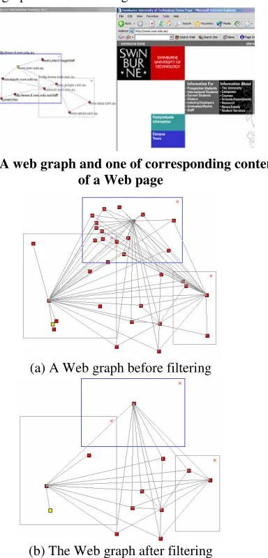
Figure 7 shows one navigation interface of a Web site. There are two parts to the interface with the left part as a
Web graph, and the right one as the content display of a Web page. Except for some abstract nodes, each node in the Web graph is linked to a URL. The node with a label called www.swin.edu.au, for example, is directly linked to the corresponding Web page, as shown in the figure. Processing the example shown in Figure 7 undergoes the following steps.
• Data extraction
The data used in this example was extracted from the Web site of the Swinburne University of Technology using the software called WebCrawler. The software accepts as its inputs a starting URL address as well as an exploration depth, and then analyzes the hyperlinks among Web pages. A URL text file containing all the extracted URL addresses of two hyperlinked Web pages is generated for further investigation.
• Filtering
The preceding filtering algorithm is applied directly to the above URL text file, or to a Web graph constructed from this file. In the graph, a node represents a Web page, and an edge indicates a hyperlink between two Web pages. With an appropriate threshold, some “noise” nodes or less important nodes are removed. An example of original and filtered graphs is shown in Figure 8.
Fig.7. A web graph and one of corresponding content of a Web page
(a) A Web graph before filtering
[image:8.595.99.254.200.469.2] [image:8.595.335.527.354.753.2] [image:8.595.88.259.501.660.2]6.2 Clustering
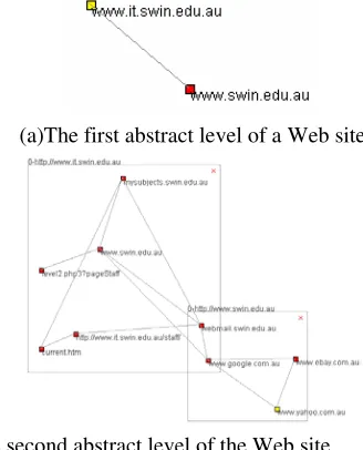
A previously presented clustering algorithm is applied to the Web graph after filtering. For simplicity, the highest abstract level of the clustered Web graph contains only two nodes as shown in Figure 9(a). With two expanded abstract nodes from Figure 9(a), Figure 9 (b) illustrates all their children nodes and corresponding edges in the second abstraction level of this Web graph.
(a)The first abstract level of a Web site
[image:9.595.87.251.169.372.2](b) The second abstract level of the Web site Fig.9. A clustered Web graph
6.3 Dynamic Adjustment
The user’s exploration may lead to overlapping windows, nodes, or labels. To improve the readability of the layout and keep the users’ mental map intact, we need to adjust the layout. The resulting layout is shown in Figure 10(b) after applying our algorithm FTA to the graph with overlapping labels illustrated in Figure 10(a).
(a) The Web graph with overlapping labels
(b) An adjustment of layout with FTA
Fig. 10. Dynamic adjustment of the Web site
7
Conclusion
In the paper, we have presented a framework for graph visualization. This framework is derived from the common characteristics of graph visualization
applications. Several new methods associated with such a framework have also been presented including filtering, clustering and dynamic layout. The filtering algorithm ranks the nodes based on the structural feature of a graph, thereby making unimportant nodes and their associated edges invisible. In contrast, the clustering algorithm superimposes abstractions of structures over a graph using the link pattern of the graph. Both algorithms can achieve the reduction of complexity of a graph layout. As far as the dynamic graph layout is concerned, an effective algorithm has been presented to accomplish the minimum adjustment of a graph layout. The prototype called PGA implementing the above three algorithms was also described, together with a Web graph case study. The future work includes the usability experiment of our approaches.
8 References
Abello, J., Pardalos, P.M. and Resende, M.G.C. (1999): On Maximum Clique Problems in Very Large Graphs.
In External Memory Algorithms (J. Abello and J.
Vitter, eds.) AMS-DIMACS Series on Discrete
Mathematics and Theoretical Computer Science, 50:
119-130.
Battista, G.D., Eades, P., Tamassia, R. and Tollis I.G. (1999): Graph Drawing: Algorithms for the
Visualisation of Graphs, Prentice Hall.
Botafogo, R.A., Rivlin, E., and Schneiderman, B. (1992): Structural Analysis of Hypertexts: Identifying Hierarchies and Useful Metrics, ACM Transactions on
Information System, 10(2), 142-180.
Bonacich, P. (1972): Factoring and Weighting Approaches to Herman Status Scores and Clique Identification. Journal of Mathematical Sociology, 2:113-120.
Bunke, H. (1993) Structural and Syntactic Pattern Recognition. In Handbook of Pattern Recognition and
Computer Vision, World Scientific Publ. Co,
Singapore, 163-209.
Bunke, H., Messmer, B.T. (1997): Recent Advances in Graph Matching. International Journal in Pattern
Recognition and Artificial Intelligence, 11: 169-203.
Card, S. K., Mackinlay, J. D., Shneiderman, B. (1999): Readings in Information Visualization: Using Vision To Think. San Francisco,Calif., Morgan Kaufmann. Chi, E.H. (2000): A Taxonomy of Visualization
Techniques Using the Data Stage Reference Model, in
Proc. Symp. Information Visualization (Info Vis’98),
69-75.
Coppersmith, D. and Winograd, S. (1990): Matrix multiplication via arithmetic progressions. Journal of
Symbolic Computation, 9:251-280.
Cristina, M., Oliveira, F.D. and Levkowitz, H. (2003): From Visual Data Exploration to Visual Data Ming: A Survey, IEEE Transactions on Visualization and
[image:9.595.52.253.485.715.2]Delest, M. I. and Melancon, G. (1998): Tree Visualization and Navigation Clues for Information Visualization, Computer Graphics Form, 17 (2), 153-165.
Dongen, S.V.(2000): Graph Clustering by Flow Simulation Mathematics and Computer Science, University of Utrecht (research carried out at Centre for Mathematics and Computer Science, CWI), Utrecht, 169,2000.
Eades, P., Huang, M.L. (2000): Navigating Clustered Graphs using Force-Directed Methods. Journal of
Graph Algorithms and Applications, 4 (3), 157-181.
Eades, P., and Feng, Q.-W. (1996): Multilevel Visualization of Clustered Graphs. In 4th International
Symposium on Graph Drawing, (Berkeley, California
USA), Springer Verlag, 101-112.
Eades, P., Lai, W., Misue, K. and Sugiyama, K. (1995): Layout Adjustment and the Mental Map, J. Visual
Languages Computing, 6:183-210.
Everitt, B. (1993): Cluster Analysis, London: Edward Arnold, third edition.
Fowlkes, E.B., and Mallows, C.L. (2001): A Method for Comparing Two Hierarchical Clusterings. Journal of
the American Statistical Association, 78 (383),
553-584.
Fu, K.S., Tsai, W.H. (1979): Error-Correcting Isomorphism of Attributed Relational Graphs for Pattern Analysis. IEEE Transactions on Systems, Man
and Cybernetics, 9:757-768.
Haber, R. B., McNabb, D. A. (1990): Visualization Idioms: A Conceptual Model for Scientific Visualization Systems. In B. Shriver, G. M. Nielson, L. Rosenblum (eds): Visualization in Scientific Computing. IEEE-Computer Society Press, Los Alamitos, 74-93.
He, W. and Marriott, K. (1998): Constrained Graph Layout, Constraints, 3 (4), 289-314.
Herman, M.S., Marshall, G., Melançon, D.J., Duke, Delest, M., and Domenger, J.–P. (1999): Skeletal Images as Visual Cues in Graphs Visualization”, Data Visualization ’99. Proceedings of the Joint Eurographics and IEEE TCVG Symposium on
Visualization, Springer–Verlag, 13–22.
Henry, T.R. (1992): Interactive Graph Layout: The Exploration of Large Graphs Department of Computer Science, University of Arizona, Tucson, 101.
Huang, M.L. (2001): Information Visualization of Attributed Relational Data. Proc. Australian
Symposium on Information Visualization, (Sydney),
143-150.
Huang, M.L., Eades, P., and Cohen, R.F. (1998): WebOFDAV – Navigating and Visualizing the Web On-line with Animated Context Swapping. In 7th
World Wide Web Conference, (Amsterdam), Elsevier
Science, 636-638.
Huang, X.D., Lai, W. (2003): Force-Transfer: A New Approach to Remove Node Overlapping in Graph Layout. In Australian Computer Science Communications. Twenty-Sixth Australasian Computer
Science Conference, Adelaide, Australia, 349-358.
Hubbell, C.H. (1965): An Input-Output Approach to Clique Identification. Sociometry (28), 377-399. Katz, L. (1953): A New Status Index Derived from
Sociometric Data Analysis. Psychometrika (18), 39-43. Kreuseler, M., Schumann, H. (2002): A Flexible
Approach for Visual Data Mining, IEEE Transactions
on Visualization and Computer Graphics, 8(1), 39-51.
Lai, W. (1993): Building Interactive Diagram Applications. PhD thesis, Department of Computer Science, University of Newcastle.
Lai, W. and Eades, P. (2002): Removing Edge-node Intersections in Drawings of Graphs, Information
Processing Letters, 81:105-110.
Leung, Y.K., and Apperly, M.D. (1994): A Review and Taxonomy of Distortion-oriented Presentation Techniques. ACM Transactions on Computer-Human
Interaction, 1 (2), 126-160.
Lourens, T. A. (1998): Biologically Plausible Model for Corner Based Object Recognition from Colour Images, University of Groningen, the Netherlands.
Lyons, K. A., Meijer, H., and Rappaport, D. (1998): Algorithms for Cluster Busting in Anchored Graph Drawing. Journal of Graph Algorithms and
Applications, 2(1), 1–24.
Marriott, K., Stuckey, P., Tam, V. and He, W. (2000): Removing Node Overlapping in Graph Layout Using Constrained Optimization, Constraints, 1-31.
Purchase, H.C., Cohen, R.F., and James, M. (1997): An Experimental Study of the Basis for Graph Drawing Algorithms. ACM Journal of Experimental
Algorithmics, 2 (4).
Shearer, K. R. (1998): Indexing and Retrieval of Video Using Spatial Reasoning Techniques, Curtin University of Technology, Perth.
Shneiderman, B. (1996): The Eyes Have It: A Task by Data Type Taxonomy for Information Visualization. In
IEEE Conference on Visual Languages (VL'96),
(Boulder, CO, 1996), IEEE CS Press, 336-343.
Story, M. D. and Müller, A. H. (1995): Graph Layout Adjustment Strategies. In Symposium on Graph
Drawing, GD’95, LNCS 1027, Passau Germany,
September, Springer-Verlag, 487-499Walischewski, H. (1997): Automatic Knowledge Acquisition for Spatial Document Interpretation, in Proceedings of 4th