Configurable Random Instruction Generator for RISC Processors

(1)

Rochester Institute of Technology

RIT Scholar Works

Theses Thesis/Dissertation Collections

12-2017

Configurable Random Instruction Generator for

RISC Processors

Krunal Mange

[email protected]

Follow this and additional works at:http://scholarworks.rit.edu/theses

This Master's Project is brought to you for free and open access by the Thesis/Dissertation Collections at RIT Scholar Works. It has been accepted for inclusion in Theses by an authorized administrator of RIT Scholar Works. For more information, please [email protected].

Recommended Citation

(2)

CONFIGURABLERANDOMINSTRUCTION GENERATOR FORRISCPROCESSORS

by

Krunal Mange

GRADUATEPAPER

Submitted in partial fulfillment of the requirements for the degree of

MASTER OFSCIENCE

in Electrical Engineering

Approved by:

Mr. Mark A. Indovina, Lecturer

Graduate Research Advisor, Department of Electrical and Microelectronic Engineering

Dr. Sohail A. Dianat, Professor

Department Head, Department of Electrical and Microelectronic Engineering

DEPARTMENT OFELECTRICAL AND MICROELECTRONICENGINEERING

KATE GLEASONCOLLEGE OFENGINEERING

ROCHESTER INSTITUTE OF TECHNOLOGY

ROCHESTER, NEWYORK

(3)

I would like to dedicate this work to my mother, my family, friends and Prof. Mark A. Indovina

(4)

Declaration

I hereby declare that except where specific reference is made to the work of others, that all

content of this Graduate Paper are original and have not been submitted in whole or in part for

consideration for any other degree or qualification in this, or any other University. This Graduate

Project is the result of my own work and includes nothing which is the outcome of work done in

collaboration, except where specifically indicated in the text.

Krunal Mange

(5)

Acknowledgements

I would like to thank my advisor, Professor Mark Indovina, for his support, guidance, feedback,

and encouragement which helped in the successful completion of my graduate research. Special

thanks to my colleagues Namratha Pashupathy Manjula Devi and Thiago Pinheiro Felix da Silva

e Lima for their work, corrections, comments and their active participation in this work. Finally,

thanks to Dr. Dorin Patru for providing access to student implementations of the various RISC

(6)

Abstract

Processors have evolved and grown more complex to serve enormous computational needs. Even

though modern-day processors share same dna with processors half century ago, verifying them

today is the huge wall to scale. Verification dominates production cycle even with advances both

in software (programming as well as CAD tools) and manufacturing (fabrication) as there are

too many test scenarios to cover. Testing complex devices like processors with manual-testing

alone in certainty missing the dead lines. Automatic verification is a great way to overcome

hurdles of manual testing viz. speed, manpower, and ultimately cost. The work described in this

paper targets verification of processors which have in-order instruction execution. Verification is

done using SystemVerilog testbench which compares output of device under test to the output of

(7)

List of Figures

3.1 System Block Diagram . . . 10

4.1 Processor Architecture Overview . . . 15

4.2 Memory organization . . . 18

4.3 Stack Organization . . . 19

4.4 Instruction word format for manipulation instructions (a) 12-bit and (b) 14-bit processor [1] . . . 20

4.5 Instruction word format for data transfer instructions (a) 12-bit and (b) 14-bit processor [1] . . . 21

4.6 Instruction word format for JUMP and CALL (a) 12-bit and (b) 14-bit processor [1] . . . 22

4.7 Instruction word format for RET (a) 12-bit and (b) 14-bit processor [1] . . . 22

4.8 Sample example for pipeline . . . 25

4.9 Pipeline stages . . . 26

6.1 Command to generate random instructions . . . 32

6.2 Flowchart for instruction generator . . . 33

(12)

List of Figures x

7.1 Errors for Test T1 - mode ’a’ . . . 47

7.2 Total error count for Test T1 - mode ’a’ . . . 48

7.3 Errors for Test T2 - mode ’a’ . . . 49

7.4 Total error count for Test T2 - mode ’a’ . . . 50

7.5 Errors for Test T1 - mode ’m’ . . . 51

7.6 Total error count for Test T1 - mode ’m’ . . . 52

7.7 Errors for Test T2 - mode ’m’ . . . 53

7.8 Total error count for Test T2 - mode ’m’ . . . 54

7.9 Errors for Test T1 - mode ’mb’ . . . 55

7.10 Total error count for Test T1 - mode ’mb’ . . . 56

7.11 Errors for Test T2 - mode ’mb’ . . . 57

7.12 Total error count for Test T2 - mode ’mb’ . . . 58

7.13 Errors for Test T1 - mode ’md’ . . . 60

7.14 Total error count for Test T1 - mode ’md’ . . . 61

7.15 Errors for Test T2 - mode ’md’ . . . 62

7.16 Total error count for Test T2 - mode ’md’ . . . 63

(13)

List of Figures xi

(14)

List of Figures xii

(15)

List of Figures xiii

(16)

List of Figures xiv

(17)

List of Tables

4.1 Processor list . . . 15

6.1 Modes for instruction generation . . . 32

7.1 Tabulation of Errors for testT1(mode ’a’) in processor kxmRISC621_v . . . 59

(18)

Forward

The paper describes a configurable Random Instruction Generator developed as part of a larger

Graduate Research project calledProject Heliosphere. The overarching goal of Project

Helio-sphere is to develop a robust, configurable, verification and validation environment to further the

study of various RISC processor architectures. The initial phase of this project was undertaken

by Krunal Mange (Configurable Random Instruction Generator for RISC Processors), Namratha

Pashupathy Manjula Devi (Configurable Verification of RISC Processors), and Thiago Pinheiro

Felix da Silva e Lima (Reconfigurable Model for RISC Processors). Indeed I am proud, and

humbled by the research work produced by this group of students.

Mark A. Indovina

Rochester, NY USA

(19)

Chapter 1

Introduction

High quality verification by directed test-benches is a very difficult task to complete within

lim-ited time constraint. Directed test-benches with simulation will get the results quickly but may

not cover areas outside the target, if a certain area is missed so are the bugs associated with

it. Also directed test-benches do not accurately simulate the real world applications a processor

might encounter. Random vector testing helps solve the problem faced by the directed

test-benches as instructions are created at random which mimic real world application and if the

verification is carried on long enough then it can be sufficiently said as verified. Another

advan-tage of random vector testing is that bugs are found faster, because of the random nature even the

bugs not thought of before can be found. The device under test (DUT) in this paper are either 12

or 14-bit in order execution processors which can be of Harvard or Von Neumann architecture.

The goal is to build a flexible test-bench such that any of the configurations can be tested and

can be scalable to even larger designs. The process is divided into 3 parts viz. random

instruc-tion generainstruc-tion, SystemVerilog test-bench and SystemC model. Random instrucinstruc-tion generator

will generate random instructions depending on the configuration specified in configuration file.

(20)

1.1 Research Goals 2

instructions. Perl is chosen as the language to produce instruction because of its text processing

abilities and other features like associative array, etc. Configuration file is also used by SystemC

model to calculate expected output for the particular instruction. SystemVerilog is chosen for the

test-bench because of its modularity and scalability. A change in test-bench will require only a

change in a particular module of SystemVerilog test-bench rather than a complete overhaul.

1.1

Research Goals

The goal of this work is to have a random instruction generator capable of generating instruction

for variety of processor which are part of test set and have provisions for other designs. This

objective is achieved as:

• Specify the basic requirements for the random instruction generator.

• Classify the processor design variations and come up with steps to create an instruction

generator to span all the requirements.

• Incorporate user switches to generate specific category of instruction, which are stored in

files compatible with processors and test-bench.

• Generate random instructions and verify two sample processor from set of eight processor,

as proof of concept.

A script is also developed to collect data from all the test runs, tabulate the data and generate

recommendations for debugging.

1.2

Contributions

(21)

1.3 Organization 3

1. A fully functioning random instruction generator is built in Perl.

2. Error detection and correction for two processors (12 & 14-bits) is carried out by various

tests to eliminate all the errors. These two processor samples are considered standard for

the rest of the set.

3. Reused a part of instruction generator script to develop result database generator, which

organizes and classify errors.

1.3

Organization

• Chapter 2: Research relating to the project outline and technology is presented in this chapter.

• Chapter3: The test environment overview with brief introduction to each component is discussed in this chapter.

• Chapter4: This chapter describes in detail processor architecture, instruction set and op-eration of the processors used in this work.

• Chapter 5: Configuration file structure along with description of each data field is ex-plained.

• Chapter6: Random Instruction Generator is described in detail in this chapter. This chapter provides a brief overview of the design followed with explanation of design choices and

function descriptions.

(22)

1.3 Organization 4

(23)

Chapter 2

Bibliographical Research

An important part of any research project is review current material related to the project

speci-fications and the relevant search results used are discussed in this chapter. The tools needed for

the development of intended work are one of the first material under research. The quest is to

validate the feasibility of the tools meeting the requirement. After reviewing related work done

with similar tools an affirmation is obtained and focus is shifted to the techniques/methods used

to accomplish project in processor verification, model design and instruction generation.

Lan-guages such as SystemVerilog, SystemC and Perl are selected and used with verificatoin tools by

Cadence to accomplish the work.

Processor verification is an intensive task, especially given that increasingly complex designs

can be designed and realized via state of the art manufacturing. In order to promote these designs,

they must be verified for correctness. Writing test cases for such complex systems manually is

quite challenging. If written to exhaustively check the system, this results in quite a large time

overhead in realizing the necessary test cases [3, 4]. This is not suitable to market the product or use it in other project as the timeline is missed. This time penalty warrants automated test

(24)

6

to generate instructions/test-cases for processor verification viz. random instruction generation

and randomizing a fixed set of test groups. The randomizing of the fixed set of test groups can

yield better results if the design has medium complexity since writing all the individual cases

will be increasing difficult. Directed manual tests have a short turn around time as they can

be easily designed for a particular case. As discussed earlier this method is not suitable for

exhaustive testing. Random Instruction testing is in stark contrast to manual testing in terms of

setup time. A random instruction generator requires a greater amount of time as randomness in

generation has to be constrained to bound tests within system design parameters and not generate

meaningless cases while at the same time reaching corners. In order to have best of both worlds

some methods researched use a novel way of randomizing part of a test case is done by making

selection of opcodes from a table but making the operands randomized [5,6]. This method gives a short setup time for the first test but will become time consuming as opcode table for all cases

need to supplied.

Random instructions can reach all the possible states including the ones not thought by the

test designer [7]. These tests when supplied with bias can give an acceptable coverage as against pure random tests [3]. Genetic algorithms are suggested and used in [8] to test a PowerPC architecture. This includes an execution trace buffer giving feed back to the bias generator, a

better set of random instructions are generate which force corner cases. Paper [9, 10] discusses generating biases with respect to the instruction groups rather than each instruction to reduce

complexity and get better coverage, which is similar to the work done in this paper. The user

has capabilities of generating a group of instruction using mode selector discussed in6.1of this paper. A different way of generating random instruction is discussed in [11]; this method uses a Linear Feedback Shift Register (LFSR) to generate pseudo-random stream of bits which is given

as input to the DUT after being verified as a legal instruction as it is possible to generate illegal

(25)

7

to estimate test length so that desired coverage is achieved without going overboard with test

runs. Paper [13] carries the bias generation a step further with much more customization e.g. test length, instruction biases, memory maps, choice of directing tests to a particular processor

element. All this customization helps target tests and also helps while debugging as only a

particular area can be identified as a problem and thoroughly tested. The research affirmed the

choice of using random instructions generator in this work, as it is versatile and can be automated

to give superior testing time.

The test environment in this work is divided into three parts: generator, model and

test-bench. This structure is chosen as it is proven, and it can be argued that the generator and

model can be combine together like in [14]. But combining the model and generator together introduces negative bias in both as they are dependent. Independently developing the model is

more flexible and brings in robustness. The model is written in SystemC as it has the modularity

and flexibility of software but can be used to model hardware, were as HDL (Hardware Definition

Languages) can do a better job but sacrifice software features of classes, objects [15]. The model is considered as reference in verification and zero errors are expected from it. Various

techniques to verify SystemC model are discussed in [16–18] viz. assertion based test, explicit state model test. The flow in verification is that the output of model is considered golden vector

and compared to DUT’s output, which depending on environment are generated and stored in a

file or verified cycle by cycle. The final piece which ties all the parts together in test environment

is the test-bench. The test-bench in this paper is developed in SystemVerilog. SystemVerilog is

chosen for its versatile nature and re-usability and the test-bench developed in SystemVerilog is

scalable as all the parts of the test-bench need not change to accommodate testing of new design

(26)

8

also tabulates results and produces graphs, an important observation made from research that

(27)

Chapter 3

Test Environment

The test environment houses all the components required for verification. Test environment is

divided into three parts Random Instruction Generator (RIG), Model and Test-bench. Random

Instruction Generator is written in Perl v5.20 and generates set of instructions in accordance

to specifications of the device (processor) under test (DUT). Model is built in SystemC and its

function is to generate reference outputs. Test bench is written in SystemVerilog and checks

DUT output for errors. Figure3.1shows the block diagram of the system.

Testing/verification starts with the configuration file. The tester or owner of DUT populates

the information fields in the file depending on the specs. Configuration file in itself is not a

functional unit but provides information, viz. processor architecture, register size, number of

registers, mnemonic-opcode pair, etc. useful for functioning of the three components. The

con-figuration file is explained in Chapter5. The RIG generates an instruction set which is read by both the model and test bench. The Model produces ideal outputs and the test bench compares

DUT outputs to model’s and reports errors if any.

The test environment has eight test samples which are mix of 12 or 14 bits, and Harvard or

(28)

[image:28.612.79.534.177.573.2]

10

(29)

3.1 Random Instruction Generator 11

the building of test environment and is proof of concept. After all the simulations have run, the

Report Database Generator (RDG) program cleans and arranges the report in final presentation

format.

3.1

Random Instruction Generator

RIG is the first to run. It extracts information from configuration file and reports of any errors

in file information. This error reporting helps so that syntax errors are avoided. Depending

on information extracted viz. processor architecture, bits, etc, instructions are generated as one

or two memory files. For Von Neumann architecture only one memory file is generated with

memory size in accordance to configuration file specifications. Whereas for Harvard, two files,

instruction & data memory file is created as shown in Figure3.1. The number of instructions are controlled by the user, if no input is associated with instruction number then a 1000 instruction

size is default. RIG also has features which protect against a number of instructions larger than

possible to fit, limit number of branch instruction so that the stack doesn’t overflow, exception

prevention as the DUT’s tested could not handle exceptions like divide by zero. Instructions

generated can be a mix of all instruction types or any combination like data manipulation, branch

- data manipulation, etc. This flexibility eases bug finding as efforts can be focused on a particular

instruction type. Since RIG calculates the result of instructions generated to prevent exceptions

and control other parameters it also generates files with registers values. The result files aid in

(30)

3.2 Model 12

3.2

Model

The model is built to emulate the processors under the test and is written in SystemC. The model

configures itself with the data extracted from the configuration file. Model takes instruction file/s

generated by instruction generator and calculates the results. Model writes out the register values

in files for each register. Model also generates files with program counter values, which helps

test-bench determine if the DUT’s flow of execution long is correct, and status flag values. Model

checks for exceptions as second safety check after RIG and other errors in instructions if any.

Output files generated are input to test-bench as shown in Figure3.1. The outputs generated by model are compared to the DUT outputs by test-bench [23].

3.3

Test-bench

The test-bench does the verification and reporting of error after simulation. test-bench is written

in SystemVerilog due to its modular nature [24, 25]. test-bench is the only common interface between different parts of environment and DUT. The test-bench receives instruction files from

the generator and provides stimulus viz. clock, instruction input. This is done by

instantiat-ing DUT in test-bench. The test-bench then monitors the output from the processor under test

and compares it to the output produced by model and instruction generator as shown in Figure

3.1. Simulation is stopped as soon as an error is detected, a report with expected values for that instruction along with registers values for a set number of instructions is generated. The

information about past results help in debugging if the error is in the current instruction or has it

stemmed from previous instruction/s. After simulation the result are fed to RDG which complies

results and produces tidied report along with ’csv’ file with error density of each instruction and

potential issues with that particular instruction. This helps in plotting graphs making it easier

(31)

3.4 Report Database Generator 13

DUT resides in the test module. Driver provides stimulus and interface provides data interface

between modules. As discussed earlier, the modular nature helps as complete test-bench need

not change with change in DUT, this makes it robust and easier to maintain [2,24]. A Perl script was written to generate the test-bench depending on specs in the configuration file.

3.4

Report Database Generator

RDG is written in Perl v5.20. After required simulations have been ran, RIG creates various logs

and reports listing error instruction and other relevant data useful in debugging. The report has

opcodes and it is difficult to visually interpret the data. To resolve this RDG inserts in a comment

stating mnemonics for the opcodes and makes other changes to make the report more visual.

RDG also complies frequency of errors and possible cause from the test-bench report, this data

is written to a CSV file making it easier to plot graphs and observe data. RDG is based on RIG

as information extraction from configuration file is the same.

RIG is discussed in the paper. Model and test-bench are part of collaborative work to develop

(32)

Chapter 4

Processor Architecture

The RISC processors used in the work are developed as part of course EEEE621 - Design of

Computer Systems supervised by Dr. Patru at Electrical Department, Rochester Institute of

Technology in Fall 2015. The specification were unique to each student according to number

assigned. All the processors were originally developed in Altera’s Quartus Prime using Verilog

or VHDL.

4.1

Overview

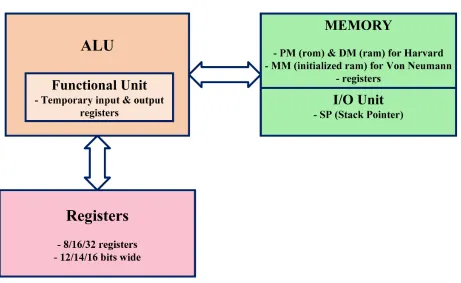
The processor architecture overview is seen in Figure4.1. It contains Memory Unit, Registers and Arithmetic & Logical Unit (ALU). Input/Output peripherals are memory mapped to the

highest 16 locations. The processors are classified into two types viz. Harvard & Von Neumann

architecture. Further sub classification is done on basis of the Instruction Word (IW) size which

(33)

[image:33.612.78.539.123.406.2]

4.1 Overview 15

Figure 4.1: Processor Architecture Overview

Table 4.1: Processor list

Processor name Architecture type Instruction word size No. of registers Status reg. size

paRISC621pipe_v Harvard 14 16 8

kxmRISC621_v Von Neumann 12 8 12

vxkRISC621_v Von Neumann 14 16 8

axtRISC621 Von Neumann 12 8 12

tflRISC621_v Harvard 12 8 12

dnm_RISC621_v Harvard 14 16 8

dxpRISC521pipe_v Harvard 14 16 8

(34)

4.2 Registers 16

4.2

Registers

Registers are used in various operations are performed and they also hold results. Depending

on instruction word size, the number of registers is limited as bits required to access them are

constrained. All data manipulation instructions have registers as operands and for write

back/s-torage. A 12-bit processor has a 3-bit register field giving eight registers (R0 - R7) whereas a

14-bit processor has a 4-bit register field giving sixteen registers (R0 - R15). A design exception

is made for the 12-bit design in flow-control instruction that register1 (operand1) size is limited

to 2-bits making 4 registers usable. This is done in order to accommodate four flag bits while

still having the same number of opcode bits.

4.3

Arithmetic & Logic Unit (ALU)

ALU is host to mathematical, logical operations, and functional unit. For most of the processors

used, mathematical operations and logical operations like shift, rotate, OR, etc are written by the

designer. Whereas multiplication and division operation are used as a unit which is generated

using Quartus’s IP wizard. The ALU in the processors used is not designed to handle exceptions

e.g. divide by zero. Functional unit houses temporary registers for both input and output. Input

operands are held in temporary registers TA and TB which can indicate register used or can hold

constant depending on the instruction. Outputs after an operation are held in temporary registers

TALUH and TALUL to hold upper half and lower half of the result respectively. Number and

(35)

4.4 Memory Unit 17

4.4

Memory Unit

The Memory Unit is monolithic for Von Neumann design as both program and data memory

reside in same memory space. Harvard design on the other hand uses separate memory space for

program and data memory. An advantage of Harvard design is that both program and data

mem-ory can be accessed simultaneously. This helps when the instructions are pipelined to increase

throughput. Section 4.6.1 discusses pipeline in detail. The memory units used are generated using Quartus’s IP wizard. In case of Von Neumann architecture design, initialized ram is used.

Initializing ram is required because program and data memory share space and the program needs

to be loaded before start of operations. The registers like Program Counter (PC), Stack Pointer

(SP), MAeff (Effective memory register) are also a part of memory unit as seen in Figure4.2. Program counter keeps track of instruction to be fetched and is incremented every cycle except

for a stall in pipeline. MAeff is calculated as addition of MAB (Memory Address Base register)

and MAX (Memory Address Index register). MAB holds the address offset and MAX holds

index which depends on an addressing mode used in a particular instruction [1]. Stack pointer points to top of stack and is incremented or decremented depending on direction of growth. Stack

in this work is defined as percentage of memory, it is made even in size by Random instruction

generator as Flow control instruction occupy two location on stack. MAeff is register not

avail-able to user, it holds the address to the location in the memory from which data can be loaded or

stored or jump location. The organization of stack is seen in Figure4.3.

Input/Output (I/O) peripherals are memory mapped for both the architecture types. The

high-est 16 locations in memory (data-memory for Harvard) are assigned to I/O peripherals. The

pe-ripheral assignment in I/O memory is user defined. A generic memory structure is as shown in

(36)

[image:36.612.73.541.85.361.2]

4.5 Instruction Set 18

Figure 4.2: Memory organization

4.5

Instruction Set

The size of opcode restricts the number of instructions possible. The processors tested in this

work have a 6-bit opcode field giving a maximum of 64 instructions. The actual number of

instructions implemented is smaller than 64. Addressing modes define how the data is fetched

or stored. For the processor used in the work operand1 (Ri) signifies addressing mode. A value

of ’0’ in the field of addressing mode indicates direct addressing mode that the offset address

present in next instruction word is the address to either jump, load or store. A value of ’1’

indicates, the final address is addition of program counter value and offset address. The rest of

the values possible for operand1 field represent register addressing mode. In register addressing

mode the final address is calculated as addition of value present in register (pointed by value of

(37)

[image:37.612.100.509.126.633.2]

(38)

4.5.1

Manipulation Instructions

Manipulation instructions modify data in registers. They are used to perform mathematical and

logical operations. They can be further divided in to types i.e. two operand instructions and one

operand plus a constant type instruction. Instruction word format for manipulation instructions

is as seen in Figure4.4. As seen in Instruction Word format register Ri is operand1 and stores result as well, Rj is second operand which can be a register or a constant value.

Figure 4.4: Instruction word format for manipulation instructions (a) 12-bit and (b) 14-bit

pro-cessor [1]

4.5.2

Data Transfer Instructions

Data Transfer Instructions transfer data to and fro between registers and memory. Since

oper-ations are register based they are likely to be loaded with value from the memory at start of

program and when a value in memory is required. These instructions are also helpful when

num-ber of values being held are greater than numnum-ber of registers, memory here provides temporary

storage for the value. Instruction word format for data transfer instructions is as seen in Figure

4.5. The offset address is stored at next memory location and is denoted as IW1 where IW0 would represent the data transfer instruction. Depending on type of addressing mode, IW1 can

(39)

Figure 4.5: Instruction word format for data transfer instructions (a) 12-bit and (b) 14-bit

proces-sor [1]

4.5.3

Branch Instructions

Branch instructions help skip or go to a different section of a program. ’JUMP’ is a branch

instruction which helps skip/jump over set number of instruction forward or backward depending

on the condition. If the condition is met the jump is taken whilst if the condition is evaluated

to be false, program continues sequentially. The conditions in ’JUMP’ instruction are set using

conditional flags. Carry (C), Negative (N), Overflow (V), Zero (Z) are four flags used as the

conditions. With four one bit flag eight unique conditions plus an additional condition when all

the flags are reset. When all four flags are reset then ’JUMP’ is unconditional and is taken.

’CALL’ and ’RET’ (return) are grouped together and are unconditional branch instructions.

Call instructions is used to execute a subroutine which is stored after program memory or other

part of program memory. Subroutines make programs neat as a piece of code to be executed

multiple time need not be replicated at the usage, instead call can be made to the piece of code.

Another use possible is to call a exception handling routine. As exception can occur sporadically

they cannot be incorporated in main program but stored else where in memory and be executed

by call the routine. Branch instructions except ’RET’ have IW1 like data transfer instructions.

(40)

4.6 Processor Operation 22

on addressing mode. ’RET’ doesn’t have IW1 or address offset as it functions to return flow

of program back to caller i.e. to instruction before which call was made. ’RET’ instruction

re-stores the values of PC and flag values stored by CALL instruction on stack during its execution.

Instruction word format for branch instructions is as seen in Figure4.6and4.7.

Figure 4.6: Instruction word format for JUMP and CALL (a) 12-bit and (b) 14-bit processor [1]

Figure 4.7: Instruction word format for RET (a) 12-bit and (b) 14-bit processor [1]

All the instructions part of processor architecture are listed in appendixIand are grouped by instruction types.

4.6

Processor Operation

Processor Operations are carried out in machine cycles. Machine cycle is a part of overall

oper-ation carried out as per instructions. An instruction operoper-ation is considered to be comprised of

four parts: instruction fetch, decode, execute and write back in the processors part of the work.

(41)

which fetches the first and next new instructions from memory pointed by program counter.

Program counter has single increment after every fetch. All the fetches from the memory need

not be instructions as depending on type of instruction second instruction word can be

mem-ory offset. Instruction decode is machine cycle 1 (MC1) in this cycle depending on instruction

opcode (i.e. after identification of instruction) operands are loaded with values from register

or constant values. It is in this step that the values loaded in operands can be forwarded from

previous instruction to resolve dependencies. Detailed explanation of dependencies is in section

4.6.1 Pipeline Theory. Instruction execution is machine cycle 3 (MC2) where the result for the

instruction is calculated. The calculated result is stored in an internal temporary register ready

to be written back in next cycle or forwarded if required. Write back is machine cycle 4 (MC3)

and is last machine cycle marking end of an instruction cycle. Here the calculated result is either

stored in the memory or the register depending on the instruction.

Processor operation is divided into machine cycle to facilitate pipelining of instruction which

is similar to a product assembly line. Pipelining increases throughput of processor by utilizing

resources efficiently.

4.6.1

Pipeline Theory

Pipeline comes from assembly line used in automobile manufacturing. In manufacturing if a

person does all the steps by himself, the steps are performed in sequence and steps ahead have

to wait for previous ones to complete. Hence a job with ’m’ distinct parts with each part taking

’n’ amount of time will take a total of ’mn’ time without pipeline. In the same example if we

have ’m’ people doing an individual task then for first whole job to complete it’ll still take ’mn’

amount of time. But after first complete job the next job will be completed in ’n’ amount of time.

This is because after completing first step first person can start working on second job’s first part

(42)

when nth person is working on nth part of first job, the first person is working on first part of nth

job. In processors machine cycle replaces a person in completing job i.e. instruction execution.

The time taken to fill the pipeline which in example meant first person doing first part of nth

job is taken only once if the pipeline is not stalled. Here in processor, a stall can occur when

the processor is waiting for an instruction to complete which uses memory and in consequence

the memory cannot be accessed.This is a problem especially with Von Neumann architecture as

there’s a single memory unit and both read-write operation cannot happen at same time. This is

an example of structural dependency where multiple instructions try to access same resources.

Structural dependencies are solved by stalling the execution of next instruction until resources

become available. If there is change in flow of program then the pipeline is reset i.e. flushed.

Flushing means completing last instruction before branch instruction then continuing on from

new address location where pipeline needs to be filled again. Hence a pipeline is useful when

program don’t have many branch instructions and such programs appear more often than ones

(43)

Figure 4.8: Sample example for pipeline

The example contains six instructions and it takes nine cycles to complete execution. The

number of cycles is nine because it takes three cycles to fill the pipeline, six cycles to execute

and three trailing cycles to complete remaining instruction execution. Fetch cycle is performed

at every clock event and hence not considered as a cycle on its own. Detailed machine cycle

for entire execution is seen in Figure4.9. As seen in sample program, first two instruction reset values in register six and seven. Instruction number three (NOT instruction) which begins at third

machine cycle has decode and operand fetch at next cycle but the first XOR instruction has not

(44)

Figure 4.9: Pipeline stages

This creates a data dependency and it’s of the type Read After Write (RAW) as NOT

instruc-tion can read the data only after XOR does write back. This can be resolved by a stall in pipeline,

but elegant way of handling this is data forwarding. Data forwarding implies that required data is

brought to the required register even before the previous instruction completes write back. With

this pipeline continues without a stall. Other dependency example is of Copy instruction. During

machine cycle six when ’copy’ instruction is in decode cycle it requires data of R6 value for

which is being calculated. So data is forwarded from ALU to the register before write back cycle

even begins. Other types of data hazards are Write after read (WAR) which occur when

instruc-tion over-writes data which is need by one of the previous instrucinstruc-tion which needs old data to

complete it’s execution and Write After Write (WAW). WAW occur when two instructions write

data to same register, this happens when instruction are out of order in execution in reference to

their issuance.

In the example with six instruction and four cycles each so the program would have taken

twenty-four cycles to complete. But with pipeline and no branch it is completed in nine cycles.

The speedup of program can be calculated as [total time taken without piepline] / [total execution

(45)

Chapter 5

Configuration File

The configuration file is key to the test environment. It contains information to setup test bench,

generate test instructions and for model to do calculations. The configuration file is populated

from the specification sheet of DUT or by the supplier of the DUT. All the numeric values are

specified in the hexadecimal format except for the percentage value. The following information

is contained in the file:

name_folder: This field gives directory name in which the files for a particular processor reside.

This is relative address to the directory test bench and resides one level below.

name: Name of the processor under test, helps locate the highest level file in directory. This

name is also used to generate instruction file, logs and reports under same name which

aids accessibility when testing multiple DUT’s.

bits: Size of instruction word for the DUT and is also the size of the registers. In the tests done

this is also the size of data bus and has two variants 12 bits and 14 bits.

(46)

28

architecture: Two types of architecture viz. Von Neumann & Harvard are indicated as, ’0’ & ’1’

respectively. This helps generator decide whether to generate a single or separate program

& data memory file.

opcode_size: Size of the field dictates number of maximum possible instruction mnemonics.

Also helps in generating instruction word and decoding in model.

operand1_size & operand2_size: This denotes the operands max size. For register-register

in-structions it gives register number used, it also can denote constant value if second operand

is constant. For the flow control instruction in processors used, Ri (operand 1) is calculated

as: (Instruction-word size) - (4 + opcode_size).

dm_size: This field only applies to Harvard architecture as it has separate data space. The

memory length is calculated as (2^dm_size).

memory_size: Total memory size available is indicated by this filed and calculated as

(2^mem-ory_size). For Von Neumann architecture this gives available size of program & data

memory combined.

pc_in_pc_relative: This information is useful in operations using program-counter(PC) relative

addressing mode. DUT design allows relative address to be calculated with respect to

current or next instruction address. A ’0’ indicates current instruction’s address is used

while ’1’ indicates next instruction’s address is used.

SP & Stack_direction: Top of stack is given by this value. Stack direction indicates the growth

of stack i.e. where next element is stored. ’0’ indicates that the elements are stored from

lower to higher address whereas ’1’ indicates elements stored from higher to lower

(47)

29

locations), this is due to the fact that 16 locations are reserved for Input/output Peripherals

(I/O-Ps) which are memory mapped for processors tested.

Stack_size: It is percentage of total memory available, in case of Harvard its w.r.t data memory

size. The size is made even as usual push on stack is two words for the processors tested.

Mapping: Mapping of mnemonics is done before specifying opcode value for given mnemonic.

Mapping is done between delimiters ’start_mapping’ & ’end_mapping’. This allows the

test environment to be DUT independent in naming the instruction mnemonic and be

flex-ible in handling various designs. The mnemonics on the left are associated with DUT and

the ones on the right are environment specific which are fixed for to be used by instruction

generator.

opcode: Here the opcodes relative to the mnemonics are to be entered. Opcodes are divided into

three categories data transfer, manipulation & branch instructions each has its delimiter

so that the instruction generator can identify different instruction and generate tests with

different combinations of instruction types.

clk_st: This value suggests number of clock cycles taken to fill the pipeline or the clock at which

first output is obtained. This is particularly useful for test bench to set reference to compare

model’s output to DUT’s for testing purposes.

DUT files:

• name_pm: This file gives the name of program memory used by DUT. This file is present

in both Harvard & Von Neumann architecture. For the latter its both program & data

memory.

(48)

30

• name_div: Divider used by the DUT.

• name_mul: Multiplier used by DUT.

• name_cnt: Counter used by DUT.

• All these files are used by the processor under test to run and perform its operations

suc-cessfully. These are also required by the test bench to list in compilation file so that the

environment instantiate or brings in correct file for to run test.

del_ld & del_st: This field provides information about whether load & store instructions are

stalled. ’1’ indicates stall after the instruction and ’0’ indicates no stall. This is used by test

bench to make result comparison at correct time clock. In usual case only Von Neumann

architecture requires stalls as instruction and data are in same memory which introduces

one clock cycle latency. Design of Harvard architecture can also stall if designer chooses

to do so.

EOF: End of file delimiter.

(49)

Chapter 6

Random Instruction Generator

RIG generates instructions used for verification and also writes the values of registers to the file.

Instructions generated at random help find bugs quicker as the tester need not manually think of

combinations. The ability to test with random instructions improves on the test case generation

time, if done manually. Hence from early stages of verification bugs or errors in implementation

can be found speeding up the turn around time. Random instructions can also test cases which

were not thought of if done manually. Manually testing all cases is both labor and time intensive

process. With multiple runs of verification, coverage close to 100 percent can be achieved with

help of the random instruction generator. The general flow of random instruction generator is

shown in Figure6.2.

6.1

Random Instruction Generator Overview

The RIG is written in Perl v5.20. Perl has powerful text manipulation capabilities while syntax

is similar to C. Text processing helps in retrieving data from configuration file and in writing

(50)

6.1 Random Instruction Generator Overview 32

Figure 6.1: Command to generate random instructions

Table 6.1: Modes for instruction generation

Mode Instructions

a All three types of instruction are generated viz. manipulation, data transfer & branch m Only manipulation instruction are generated

mb Manipulation and branch instruction are generated md Manipulation and data transfer instruction are generated

generator is made configurable so that as the input configuration changes, it adapts to it. To

achieve this robustness the instruction generator is kept modular and the calculations are kept

generic and depend on the input configuration file. The instruction generator also has built in

error reporting. If the input configuration file has error in input data syntax or is missing data

field then the user is notified of such error with prompts on how to fix the errors. The command

to run the instruction generator is seen in6.1:

The minimum input requirement is a configuration file 5, as it contains all the vital infor-mation to proceed with the instruction generation. The other input parameters are number of

instruction and ’mode’. RIG can generate user defined number of instructions. The default value

for number of instruction is 1000 in this work, to ensure that even without being supplied with

number of instruction the RIG works. The input of ’mode’ is to compare generating a certain

type of instructions, table 6.1 describes 4 modes. The flow of RIG is seen in Figure 6.2. The process begins with extracting information from configuration file done by Extract function. The

information extracted gives memory limits and information on segments inside memory like

stack, I/O space. With the processor architecture known the next function, ’memory_set’, knows

(51)

func-6.1 Random Instruction Generator Overview 33

(52)

6.2 ’extract’ Function 34

tion sets the memory limits for next functions to continue the operation. The ’filler’ function

fills the memory with zeros in locations which will contain data later on as the instructions are

generated. It also fills memory locations with ones which are not written on by generator. The

’gen’ function is responsible for generation of instructions. It does so by calling sub-functions

viz. manipulation_gen, data_transfer, branch. Instructions generated are written to the file by

the ’writeout’ function. ’reg_out’ function does the task of writing out values of registers to file

to be used by testbench. The functions shown in Figure6.2are discussed in detail in following sub-sections.

6.2

’extract’ Function

The ’extract’ function takes the configuration file as an input and extracts all the information

about a particular processor. All the values inside the configuration files are hexadecimal, while

calculation in RIG are in decimal. Hence all the values are converted into decimal. The values

are extracted line by line from the configuration file. Any line beginning with ’#’ is considered a

comment and is ignored. All the configuration file reside in the ’configuration’ directory which is

one directory level below the RIG. All the extraction of information is done via Regular

Expres-sions (regex) [28]. The regex match and extract a part of a string depending on the criteria given. Mapping of instruction and opcode for mnemonics are written between delimiters e.g. for data

transfer instructions ’start_data_transfer:’ and ’end_data_transfer:’ are the start and end limiters

respectively. The delimiters helps in determining a section of data and hence the sections can

be in any sequence in configuration file. Absence of either opening or closing delimiter causes

an error so that errors in configuration file are avoided. ’EOF’ marks the end of file and it is

(53)

6.3 ’memory_set’ Function 35

6.3

’memory_set’ Function

The ’memory_set’ function sets up the memory. The function first calculates the maximum

mem-ory from the information in configuration file. The value of field ’bits’ from the configuration file

is taken as power to base 2 to calculate maximum memory possible from that bit size. Here in

this work memory for a processor is calculated with its bit size. For Von Neumann architecture

only one memory with the calculated size is created, whereas for Harvard architecture two

mem-ory with same size are created to serve as program and data memmem-ory. But the random instruction

generator has provision to support user defined memory which can be smaller or greater than

calculated memory size. This custom memory size can be supplied for both program and data

memory, if present.

The stack is given as percentage of total memory size or data memory size for Harvard type

processors. While calculating memory locations to be reserved for the stack care is taken that

the value is even. An even value is chosen as instructions like CALL (branch instruction) use

two stack locations one for storing flags and program counter value. To verify the supplied

number of instructions can be generated reserved memory is calculated. If the space in memory

after subtracting reserved space is greater than desired number of instruction only then RIG

proceeds further. In case of instruction number exceeding the memory space available a warning

is reported along with the memory space available and execution of generator is carried with

maximum memory space possible. Reserved memory is calculated as addition of stack memory,

I/O space if memory mapped, subroutine space, data space in case of Von Nuemann architecture

and two additional memory locations. The subroutine space in this work is 40 memory locations

but can be changed. Data space is reserved in case of Von Neumann type processors so as to

allow instruction to write and read from memory location which would be impossible to do if

(54)

6.4 ’filler’ Function 36

there is separate data memory. Two memory location are reserved as those locations contain one’s

stored which serves as end of program for testbench at which simulation can be stopped and is

completed. At the end of this function memory space is divided accordingly and instructions can

be generated. A typical memory layout for Von Neumann type is shown in Figure6.3.

6.4

’filler’ Function

This function serves as building error checking in memory while generating instructions. It fills

the arrays with character ’k’ which hold data to be written to memory to both program memory

and data memory or just to one memory in case of Von Neumann architecture design. The

character is chosen at random and it is written as visual aid. Since no address value or opcode

at the location will have character ’k’ it helps catch error in generated instructions if any. Later

on during write out to file this helps in filling memory space with ones where ’k’ is found. The

locations with ones as data, can be address offset if preceded by a associated valid instruction

opcode. At other locations a string of ones mean that the location is not defined. Also this string

of ones can help detect branch error when the instruction word reads a string of ones instead of a

valid instruction.

6.5

’gen’ Function

The ’gen’ function is the largest function written. It is responsible for generation of instructions

and also prevention of exceptions as the processors in this work exclude exception handling.

The ’gen’ function is also made modular so that the development and maintenance in future is

relatively easier. The instructions are randomized in this function. The mnemonic and opcode

(55)

6.5 ’gen’ Function 37

(56)

keys is selected via ’shuffle’ function which is part of Perl’s ’Util’ library which contain general

purpose subroutines. The ’gen’ function is also responsible for generation of a certain set of

in-structions depending on user input, with ’a’, i.e. all inin-structions, being the default option. A set

of only branch or data transfer instructions is not generated as branch instructions need some

in-structions to branch to. And just branching the flow of execution will not reveal any dependency

error which are caused by other instructions when in a combination with branch instructions.

Similarly data transfer alone will not yield much information about errors, as reading or writing

garbage value cannot be verified if the same arbitrary value is written and read back again. Hence

both branch and data transfer instructions are paired with manipulation instructions to provide

data to read or write as well as good variation for dependency check when branching. The ability

to generate instructions with only certain desired types help in debugging a desired part of the

processor design as errors reported will be exclusively from the desired types of instructions. The

function is also intelligent to detect if a branch is to an undefined location. In such event branch

operation is skipped and replaced with one of the manipulation operations. The data transfer is

not chosen in case of an invalid branch because even data transfer from that location will be

un-defined. After choosing a random instruction ’gen’ calls sub-function to generate manipulation,

data transfer or branch instructions.

6.5.1

’manipulation_gen’ Function

This function to generates manipulation instructions and calculates results for the generated

in-struction. This function then applies another layer of randomization by randomly selecting

reg-isters for the operation. In case of an instruction with constant as the second operand, the register

number generated for operand2 still applies as the field size is same. After calculating result of

instruction flags need to be set according to the result. The flag assignment is done by ’CNVZ’

(57)

prevents code duplication. Another function ’compactor’ resizes the result to fit the width of

instruction word of a particular processor. The resizing of the result is required for certain

in-structions as the entire result is not stored to destination, some information is contained in flags.

An example of such result resizing is adding two 12-bit operands in a 12 bit processor yields a

13-bit result of which the most significant bit (MSB) is carry. Thus result is clipped to 12-bits

while ’CNVZ’ function already has carry information. The last function to be called to generate

opcode for the instruction generated is ’iw1_gen’. The ’iw1_gen’ function generates instruction

word in format specified by configuration file for a processor. The opcode (instruction word)

gen-erated is stored in an array later to be written in memory. Other information stored is resultant

register values.

6.5.2

’data_transfer’ Function

The ’data_transfer’ function also generates random values for the operands. In the case of data

transfer instructions, i.e. LOAD & STORE, operand1 represents the addressing mode. Operand2

is the source or destination of data when the operation is STORE or LOAD respectively. The

data transfer instructions are two instruction words wide for the processors under the test. The

first instruction word which defines the instruction is followed by the address offset. The final

address is obtained as an addition of the address offset and base register address (MAB). The

base register address is defined by the addressing mode which is the value of operand1. A value

of ’0’ represents direct addressing mode which implies that the final address is equal to the value

of address offset. A value of ’1’ represents PC relative addressing mode and the final memory

address is calculated as sum of PC value and address offset. The values from two onwards to the

highest number specified by operand1 field (e.g for 12-bit processor it is 7) represents register

addressing mode. The final address is equal to the value held by the register. To generate the

(58)

according to the addressing mode, MAB is subtracted to give the offset address. It is ensured

that STORE doesn’t happen to a program memory location in Von Neumann architecture. This

makes sure that the program is not corrupted. If the final memory address is out of memory

bounds then the previous value of operand1 (addressing mode) is changed to one that’ll fit the

memory range. Also since data transfer instructions are allowed in subroutines and before JUMP

a caution is exercised result of which the instruction is skipped if only one memory space is

available at the end of routine or before jump. A provision is also made to put a random value if

a load operation is from a location which is undefined. At the end of the ’data_transfer’ function

a call is made to ’wi1_gen’ to generate the instruction word.

6.5.3

’branch’ Function

With a branch instruction selected by ’gen’ function the ’branch’ function takes over to perform

checks and to generate an instruction. Just like data transfer instructions, jump location or

sub-routine call addresses are calculated according to addressing modes. For JUMP instruction a

check if the jump is within the program is performed if it is register addressing mode. If the

jump is outside the program, then other registers are checked for providing the address value

within program space. One of the other addressing modes is chosen if the previous check fails.

For direct and PC relative addressing mode jump size is fixed depending on total number of

in-structions. Depending on the jump size, the address offset is calculated. The jump size is fixed

so that long jumps are avoided which would lead to skipping most instructions making overall

test shorter and would increase test time as testing all combinations will take more number of

tests. Jump can be taken in a forward and backward direction. A backward jump is of particular

interest in instruction generation as it must contain a forward jump to jump ahead of backward

jump’s instruction location else it’ll result in infinite loop. Hence to generate a backward jump a

(59)

6.6 ’write_out’ Function 41

is a exit jump to avoid infinite loop. The third jump, i.e. the backward jump, takes flow before

the second jump which jumps ahead of it.

The ’call’ instruction can have its subroutine length as maximum of 10 instructions if it’s

at top level in nested calls. The nested call can have subroutines with maximum length of 6

instructions. This is done because subroutine space is limited and maximum instruction variation

should be checked in a test. A depth level of three nested calls is allowed in this work, depth level

can be increased with change in the code. It is made sure that there is a ’return’ instruction at the

end of a subroutine block to take the flow of execution back to the main program or a subroutine

higher in nested call. The ’branch’ function also calls ’iw1_gen’ to generate the instruction word.

6.6

’write_out’ Function

The write_out function writes the instructions generated and the register values for those

instruc-tions which were stored in arrays to files. The instrucinstruc-tions generated and corresponding resultant

register values are then stored in an array as it makes accessing the data and manipulation easier.

Also, writing a single value in a file would mean having write handle (pointer) open during the

entire writing process increasing risk of data being mishandled. For Von Neumann architecture

only one file named ’memory.t’ is created and is written into. For Harvard architecture this file

also serves as program memory and ’data_memory.t’ is the data memory file. These memory

files are created in directory named ’heliosphere’ which is one directory level below and hosts

(60)

6.7 ’reg_out’ Function 42

6.7

’reg_out’ Function

The register values are written in same directory as RIG by the ’reg_out’ function. The file name

is same as the register name e.g. for register 0 its ’R0.t’ , for stack pointer it is ’SP.t’. All the

locations for memory or register may or may not have data in them, those locations are filled

with binary string of one. A separate function is created because the decision to write the register

values out was made later in project to help with verifying the model’s output. This extra set

of values helps ensure that model gave correct values while building the test environment. Also

(61)

Chapter 7

Results

The results are obtained after running simulations. The Report database generator (RDG) then

makes visual changes to the reports and generates ’.csv’ files to facilitate graphing. During

first run of simulations, status flag related errors are observed to dominate. Thus majority of

simulation runs are cut short and other errors are not reached. This mandated a second test with

status flags changed to follow a standard according to the specifications. Test two yielded variety

of errors which give helpful insight into design errors and dependencies. The results of two sets

of tests, T1 and T2 are collected and graphs plotted to give visual representation and overview of

problem area in DUT design.

The RDG is also equipped with feature to classify error into four categories viz, status flag,

Program counter, Implementation errors and undefined registers.

Status_Flag: These are the errors in which the status flag don’t match the model’s output. These

errors are prevalent as some design constraint in course EEEE621 - Design of Computer

Systems were left at programmer’s discretion, which resulted in variations in status flag

implementation.

(62)

44

A wrong branch results in this error, the cause can be wrong memory address calculation

or incorrect return address.

Implementation_Error: When a register value doesn’t match the expected value it is

consid-ered as implementation error. The probability of the instruction’s functionality is very high

if there is mismatch between expected and observed register value. A few cases where the

error may not be implementation related are when a branch is taken to an incorrect location

or a return to an incorrect memory location. But this field give a good start in debugging.

Undefined_reg: This type of error is recorded when a don’t care (’x’) logic value is observed.

The usual cause of this error is uninitialized register value on reset or wrong data size

transactions between registers.

The above classification of errors are a helpful aid in debugging process as a start point. An

Excel spreadsheet file is created to group data, obtained from test-bench, in a table. This excel

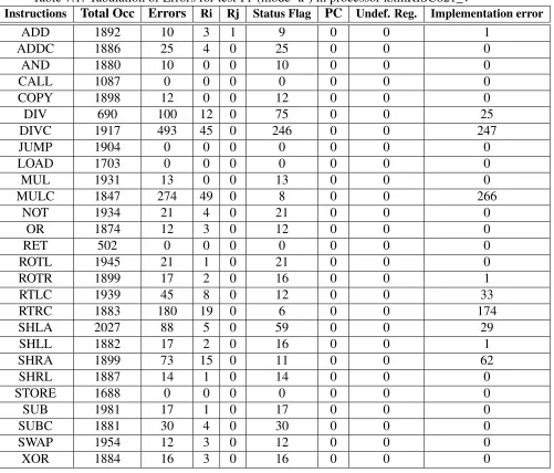
file is used to create graphs using Matlab, presented in IV. The table has a dependency field related to two operands i.e. Ri, Rj. This field helps identify total occurrences on which an

error coincided with a possible register dependency. This being not a perfect number, can give

insight into a possible register dependency not being resolved in the design. Another important

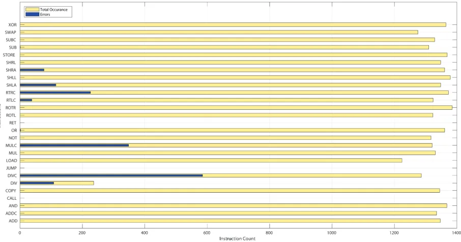
observation presented to user is total occurrence of an instruction versus total number of errors

of that instruction. An example of a test results in tabular form is in table7.1which is test T1 in mode ’a’.

Two set of tests are run for a DUT. Each test set has a subset of four test corresponding to

four test modes as explained in6.1. So a total of 8 tests are run for a DUT, each test has 1500 iterations with 1000 instructions each. An example of a script to run 1500 test for a DUT in

mode ’a’ is as follows:

(63)

7.1 Mode ’a’ 45

2 rm . . / r i s c /T e s t _ R e s u l t.t

3 rm . . / r i s c /c p l o g.t

4 rm . . / p l/p e r l.l o g

5 rm l o g.t

6 cp . . / c o n f i g u r a t i o n /c o n f i g u r a t i o n _ 2 _ k x m.t x t . . / c o n f i g u r a t i o n.t x t

7 p e r l . . / t e s t _ g e n/t e s t _ g e n r.p l −l e n 4 # c a l l t o t e s t b e n c h g e n e r a t o r

8 f o r i i n { 0 . . 1 4 9 9 . . 1 } 9 do

10 cd . . / p l/

11 p e r l g e n _ v t.p l −c o n f i g c o n f i g u r a t i o n .t x t −mode a > p e r l.l o g # c a l l t o i n s t r u c t i o n g e n e r a t o r

12 cd . . / p r o c e s s o r/

13 make

14 cd . . / r i s c

15 . /sim.c s h −r −ng −s v −r u n

16 e c h o "Test $i"

17 18 done

19 cd . . / p l

20 p e r l e r r o r _ r p t .p l −c o n f i g c o n f i g u r a t i o n .t x t −mode a −num 1500 21 # c a l l t o R e p o r t d a t a b a s e g e n e r a t o r

Listing 7.1: bash version

The results are grouped into four categories depending on mode. Each mode has two tests T1

& T2, T1 being results with original DUT design and T2 with status flag modification. Results

for a processor ’kxmRISC621_v’ are presented and discussed in following sections.

7.1

Mode ’a’

In mode ’a’ all the instructions are generated and it gives an overview of errors in the design.

This mode can be used at the start to find the group of instructions with most errors and target

simulation to that group using different simulation mode. This mode is also useful when most of

(64)

7.2 Mode ’m’ 46

7.1.1

Mode ’a’ - Test T1

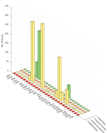
As discussed earlier this test is with no corrections to the status flags. From figure7.1 it is seen that the status flag error are present for majority of instructions. Errors related to implementation

errors are prevalent as for ’Mul’ & ’Mulc’ as well as ’Div’ & ’Divc’ instructions the design saves

the result in a different way than the standard defined in this work. Other implementation errors

are due to an instruction incorrectly implemented e.g. SHLA implementing left shift incorrectly.

It can be seen that with help of the figure representing errors it is easier to start debugging .

Figure 7.2 shows