Graph-based Performance Estimation on Customized MIPS Processors

Theses

7-2018

Graph-based Performance Estimation on

Customized MIPS Processors

Saaim Valiani

[email protected]

Follow this and additional works at:https://scholarworks.rit.edu/theses

This Thesis is brought to you for free and open access by RIT Scholar Works. It has been accepted for inclusion in Theses by an authorized administrator of RIT Scholar Works. For more information, please [email protected].

Recommended Citation

Graph-based Performance Estimation on

Customized MIPS Processors

Saaim Valiani

July 2018

A Thesis Submitted in Partial Fulfillment

of the Requirements for the Degree of Master of Science

in

Computer Engineering

Graph-based Performance Estimation on

Customized MIPS Processors

Saaim Valiani

Committee Approval:

Dr. Sonia Lopez Alarcon Date

Advisor

Department of Computer Engineering Rochester Institute of Technology

Dr. Marcin Lukowiak Date

Department of Computer Engineering Rochester Institute of Technology

Dr. Andres Kwasinski Date

To my parents and my sisters. Thank you for always supporting me throughout

my life and reminding me to smile and be happy.

To my advisors, Dr. Lopez Alarcon and Dr. Lukowiak. Thank you for the

continued support and all of the help and feedback you provided throughout my

time in college. This would not have been possible without you.

To my best friend, Cody Tinker. Thanks for being my best friend. You have

always motivated me to do my best and provided encouragement through tough

times.

To my other best friend, Jake Teitsworth. Thanks for all the support and

advice you have provided. You are a one of a kind person and the main reason I am

still sane.

To my third best friend, Yash Nimkar. Thanks for being my brother. You

helped make life so much easier by constantly providing help and support in so

Abstract

The desire for greater processor performance with shrinking technologies and

increas-ing heterogeneity, leads to a need for improvement in performance estimation. Beincreas-ing

able to estimate the performance of an application without needing to implement the

application on the available hardware and soft-core choices can decrease development

time and help expedite the process of choosing which platform would be the best

choice to use for development.

This thesis work focuses on using a graph-based description of an application to

estimate performance. By using a graph-based approach, the need for a hardware

specific implementation is eliminated and the design space is simplified. Breaking

down an application into a graph allows a new approach review to be taken as nodes

of the graph can be assigned to levels in the pipelined architecture. This research uses

pipelined customized Instruction Set Architecture (ISA) processors as the platform

choice. The customized ISA soft-core processors allow the user more control over the

resources used in the processor and provides a viable hardware/software choice to

demonstrate the capabilities of the graph-based approach.

The testcase applications used were the Dot Product, the Advanced Encryption

Standard (AES) application, and the AES with TBox application. The results of

this work show that performance can be accurately estimated on a customized

pro-cessor using a graph-based approach for the application with accuracy ranging from

Signature Sheet i

Acknowledgments ii

Abstract iii

Table of Contents iv

List of Figures vi

List of Tables vii

Acronyms 1

1 Introduction 3

2 Related Work 6

3 Proposed Methodology 12

3.1 Background and Basis of Research . . . 12

3.2 Implementation Flow . . . 14

3.3 Graph-based Approach . . . 19

3.4 Applications . . . 25

3.4.1 Dot Product . . . 26

3.4.2 AES . . . 26

3.4.3 Instructions . . . 30

3.5 Preliminary Analysis . . . 31

3.6 Experimental Setup . . . 37

4 Results 38 4.1 Dot Product Results . . . 40

4.1.1 Dot Product Results Analysis . . . 43

4.1.2 Dot Product Results Discussion . . . 44

4.2 AES Results . . . 46

4.2.1 AES Results Analysis . . . 49

CONTENTS

5 Conclusion 52

3.1 Flow diagram of Customized Soft Processor[4] . . . 14

3.2 Portion of Example Processor Architecture . . . 16

3.3 Example Pipelined Architecture [5] . . . 19

3.4 Example Dataflow Graph [5] . . . 19

3.5 Example Reduced Graph [5] . . . 20

3.6 Example Pipelined Architecture Reduced Schedule [5] . . . 22

3.7 Example Pipelined Architecture Execution Schedule (E - Epoch) [5] . 23 3.8 128bit AES Standard Implementation Initialization . . . 27

3.9 128bit AES with T-Box Implementation Initialization . . . 29

3.10 Sim. Observation for Dot Product with Input Vectors [1, 3, 5] and [4, 2, 1]Iteration- Current iteration of the main ’for’ loop in the applica-tion Input - Current element being processed from the input vectors Mathematical Output- Output of dot product between current el-ements of input vectors . . . 32

4.1 Example of Span Determination . . . 39

4.2 Scheduled Graph for 2 vector, 1 element Dot Product Application . . 40

4.3 Performance Estimation of Pipelined Dot Product . . . 44

4.4 High Level Dataflow Graph of AES . . . 46

4.5 High Level Dataflow Graph of AES with TBox . . . 47

List of Tables

3.1 MIPS Instruction Usage per Application . . . 30

4.1 Performance Estimation of Pipelined Dot Product . . . 43

AES

Advanced Encryption Standard

FPGA

Field Programmable Gate Array

GPP

General Purpose Processor

HDL

Hardware Description Language

HLS

High Level Synthesis

ISA

Instruction Set Architecture

ISE

Integrated Synthesis Environment

LUT

Lookup Table

MIPS

Acronyms

SDK

Introduction

As new devices and technologies aspire to provide better performance, there is a

greater need for performance estimation and new design tools. Researching a

graph-based approach for estimating performance would be beneficial to the current paradigm.

As it currently stands, in order to estimate performance for an application, either a

hardware specific or a software specific implementation for that application can be

considered.

Consider a system where hardware or software choices are available and an

appli-cation with several computations or several tasks is on-hand. We propose that if an

evaluation is needed to determine which choice would be best for the performance of

the application, this can be approximated by using a graph-based approach and could

greatly benefit this area of research. In other words, using a graph-based approach

would remove limitations that currently exist by reducing the design space.

This research focuses on estimating the performance of algorithms on customized

Instruction Set Architecture (ISA) processors [4]. These are soft-core processors that

are designed with a customized ISA to reduce the number of resources used. The

purpose of our work is to allow researchers a quicker method of determining the

performance of an application which facilitates making design choices during the

development process. Consider the development situation in which a processor is

CHAPTER 1. INTRODUCTION

(FPGA) as a hardware choice. FPGAs are a popular choice as they are reconfigurable

and quite versatile. An FPGA board can include a General Purpose Processor (GPP)

on which a software kernel can be implemented to be able to perform software tasks.

These processors are also known as hard processor cores. An alternative to this is

using a standard soft processor, such as MicroBlaze which is developed by Xilinx [7].

This type of soft processor is designed for use on reconfigurable hardware and comes

packaged with a Software Development Kit (SDK). There also exists a third option,

which is the focus of this research: to implement a customized soft processor which

uses specifically tailored resources. Doing so allows the user to be able to only utilize

the needed resources to implement a set of instructions out of the whole ISA and

therefore save overall resource utilization.

In order to be able to make a choice between the different options, we would

like to have a method for estimating the performance of each option without having

to implement the application on each choice every time. This can be done using

a graph-based methodology. In other words, using a graph-based approach would

remove limitations that currently exist by providing more freedom and possibilities

for estimation. Customized soft-core processors are used to provide a platform to

estimate performance on. The reasoning for choosing this approach over the other

choices is because it provides us with a processor of which we have control. We

don’t need to research the estimation of the performance of software kernels running

applications because the application can just be run and then the execution time can

be examined. Estimation of performance on hardware is an aspect that has been

explored [2]. The customized processors can provide a proper platform for which

estimation of performance has not been explored.

One major feature of this research is that the graph of the application can be

extracted at the C language level. This avoids the need for having to go to the

can be applied to many more applications. As it pertains to our research, we check

our performance estimation in two cases: varying the input size and varying the

Chapter 2

Related Work

A graph-based approach to estimating performance remains an area that has not

been researched, particularly in relation to customized ISA processors, and therefore

can be a valuable resource. There has been research performed in similar areas that

are related to performance estimation. This research is proven to be valuable to

understanding the research area of performance and estimation and the benefits it

brings to advancing technologies.

Research has been conducted in the past about performance of pipelined

archi-tectures on FPGAs pertaining to liner algebra algorithms [2]. The previous research

presented a mathematical model that can provide performance estimations of

appli-cations on hardware. These models were based on the use of available resources.

Pipeline sizes to achieve maximum performance were also determined. The

math-ematical models were compared to actual simulated hardware implementations to

verify accuracy, which is similar to the approach that was used in the current

re-search to provide a point of comparison. This rere-search pertains more to the hardware

implementation choice that researchers can take as it relates directly to FPGAs. Our

research estimates performance based on a graph extracted from a software

imple-mentation of an application and the use of a customized ISA processor as a platform.

So, though we do use pipelined architectures and mathematical applications, our

under-stand possible techniques for performance estimation and was also used a method of

verifying that performance estimation can be done using a hardware specific

imple-mentation.

Other research that has been conducted is the Aladdin project [1]. This project

attempts to provide performance and energy advantages by using an accelerator

simu-lator. This enables larger exploration of the design space, but a custom datapath and

control logic would be needed for the algorithms. Though it does allow quick

mod-eling without generating RTL, the restrictions in terms of requirements are present.

The Aladdin project is an example of a hardware specific implementation. It

pro-vides increased performance advantages, but requires the implementation of hardware

specific technologies such as an accelerator. This research was used as background

information pertaining to what aspects affect performance in hardware and how

per-formance can be increased. The methodology proposed in this research was not taken

because it was a hardware specific approach and relates to increasing performance

rather than estimation.

Another aspect of research previously conducted looks at a different way of

vi-sualizing performance. The Roofline Model relates the performance of the processor

to off-chip memory traffic [3]. This is done because off-chip memory bandwidth is

usually the limiting resource in terms of performance. The performance modeling is

done by directly interacting with hardware to determine the traffic. This is, therefore,

another example of a hardware specific implementation. The processor would need to

be physically present and monitored to determine the traffic of the off-chip memory.

The traffic is monitored and mathematical models are created to estimate

perfor-mance from the observations. The difference between this previous research that

was conducted and the research being proposed is that the previous research did not

use a graph-based approach. By using a graph-based approach, the current research

CHAPTER 2. RELATED WORK

The previous research is useful in helping to determine how to estimate performance

for hardware specific implementations.

Research has also been done to be able to estimate performance of an application

based on the register-transfer level descriptions of the application [8]. The idea is

that typically register-transfer level is given for existing hardware components. If

performance can be estimated from that, it can apply to a variety of situations. This

approach was not used because it is too low-level for the implementation we had in

mind. Our goal is to be able to estimate the performance of an application from

a high-level description. It is also not a method that can be too easily expanded

for tasks such as testing different input sizes or different implementations, something

that the graph-based approach allows us to do.

Performance estimation of applications on microcontrollers [9] is another aspect

that was looked into when performing background research. Though this approach

is specific to microcontrollers, it provided some inspiration for our current research.

In this methodology, each C language operation’s execution time was measured for

different microcontroller architectures. Doing so allows loops and loop bodies to

ana-lyzed and performance to be estimated. This approach was taken into account when

the cycle counts per epoch were determined in our research since it is a simple and

straightforward method to implement. Though this research does not fully pertain to

our research because the platform that was used was microcontrollers, it did provide

a good route to consider as it pertains to estimation.

Another research effort conducted was to be able to estimate performance for a

high performance computation workload by preforming a sensitivity analysis [19]. The

idea is that a sensitivity analysis can be preformed to determine which parameters

in an architecture (such as number of threads or memory) cause the most change in

performance. Using this analysis, mathematical models can be created to estimate

analysis. This research route was not taken as it does not relate to a graph approach,

but it did present the idea that the performance of an application can be particularly

sensitive to one part of the architecture over another.

Research on a method of estimation relating to memory has been conducted to

model performance of hierarchical memory systems [20]. The model estimates

per-formance of a multi-level hierarchy using single level cache statistics. The idea was

to develop an analytical model based on a decision graph. Each node of the graph is

a decision related to memory (cache miss, cache hit, etc.). By assigning probabilities

and costs to each branch of the graph, an analytical model can be constructed based

on the probability of each branch. The execution time can then be found by following

all paths in the decision graph and preforming the summation of the execution times

of the graphs weighted by probability. This research showed another mathematical

method for estimating performance but utilized probabilities. The interesting aspect

is that it used a graph to do so. Though this research does not relate all too much

with the proposed research, it showed that a form of a graph approach can be taken

to estimate performance.

Research has been conducted on a graph analytics approach for a manycore

pro-cessors [10]. The idea is to be able to systemically optimize algorithms by identifying

frequently-used optimization strategies from various implementations and applying

it to a structured methodology. So therefore, altering a structured algorithm based

on optimization strategies. This research was investigated to provide some more

background on graph based approaches to applications and algorithms. Due to the

concept of this research differing in various aspects from our current research

(many-cores being used as the platform, not performance related, etc.) this approach was

not used. It did, however, provide good insight as to how graphs can be used for

various tasks and how useful they can be.

CHAPTER 2. RELATED WORK

[5]. The idea was that a full graph (known as a dataflow graph) describing the

algorithm could be designed based on a pipeline of operations. The full graph would

then be represented in a reduced graph format based on the number and type of

operations at each level of the graph. An execution schedule can be derived by

observing the pipeline along with the dataflow graph and a reduced schedule could

also be determined from the reduced graph. This methodology is explained in more

detail in section 3.3. This methodology was used as a basis of the current research and

this paper as it is used to create the graphs from which the performance is estimated.

The reasoning for using this graph-based approach as compared to others revolves

around the ability to easily calculate the epochs in a graph. Further explained in

section 4, being able to find the span of a graph quickly and therefore being able to

know how many epochs the execution schedule of a graph takes was considered to be

very valuable. From this aspect, the idea was developed to assign some sort of cycle

count to each epoch (since it represents how the graph is scheduled on the platform)

to be able to estimate the performance of the application.

Another basis of this paper is specifically estimating performance on a customized

MIPS ISA processor. Research was conducted on how to design customized ISA

pro-cessors using High Level Synthesis (HLS) [4]. The customized propro-cessors provide a

fully controlled environment to test the performance estimation of the software

im-plementation of the application. The processors allow for lower resource consumption

(further explained in section 3.2) by allowing a method of customizing the ISA used

for the application being implemented. This in turn would be expected to increase

the performance of the application. The reasoning for using this approach as a basis

for this research is that it provides a hardware and software platform that has not

been studied for performance estimation. Hardware specific implementations have

al-ready been researched as it pertains to performance estimation, thus exploring a new

simplify the design space. In addition, since this platform is already expected to have

greater performance than traditional methods, it allows for performance estimation

Chapter 3

Proposed Methodology

3.1

Background and Basis of Research

As was stated in Chapter 2, the platform used to conduct the research on

perfor-mance estimation using a graph-based approach was a customized ISA processor. A

customized ISA processor is a soft-core processor that provides the user with greater

control of the resources used. By being able to control the architecture used for the

specific application in question, the designer has the ability to select the instructions

that need to be implemented as opposed to implementing all of the instructions. This

allows for lower resource utilization. This aspect is further explained in section 3.2.

Customized processors also help to facilitate greater exploration of the design space

since the researcher now has control over aspects of the processor that are generally

not too accessible.

The basis of this research lies in performance estimation. This type of estimation

is a very important type of analysis because if done right, it can greatly help to

reduce development and analysis time. As technology evolves and both software

and hardware tasks become increasingly complex, being able to more easily know

which development route to take can save a lot of time and resources. In addition,

being able to predict and estimate how an input change can affect the performance

questions such as how long an application will take for different input sizes without

having to run the experiment for all sizes or if adding new instructions can create a

more robust architecture that can support multiple applications is the foundation and

formation of the research that was conducted. If a researcher can properly estimate

how long an application will take to run for a small input size and easily be able

to apply that to larger input sizes with a quick analysis and not have to actually

carry out the experiment, the savings in time and resources can become increasingly

great. Thinking along these lines, if a researcher changes their implementation of a

resource demanding application and knows what changes that entails in the estimation

analysis, being able to simply make those changes in the analysis and not have to run

the new implementation to obtain the performance of the implementation would result

in a great reduction in workload. Not only would this analysis reduce the workload

and resources needed, it would also allow researchers to also know which type of

design platform would be best to use. If the research can reduce the requirements

for testing multiple versions of an application on multiple design choices the analysis

would prove to be quite valuable.

To conduct this analysis, we want to be able to estimate the performance of

an application by extracting a graph from the software kernel which represents the

application. Extracting it from this level would not require the software to be executed

and a design decision can be made on which type of processor would be ideal for such

CHAPTER 3. PROPOSED METHODOLOGY

3.2

Implementation Flow

Figure 3.1: Flow diagram of Customized Soft Processor[4]

Figure 3.1 displays the implementation flow of a customized soft-core MIPS

proces-sor separated into the three main stages of the process, the Software Implementation

Flow, the Hardware Implementation Flow, and the Performance Evaluation [4]. The

goal of our work is to test the accuracy of graph-based performance estimation on

pipelined processors generated this way. To properly be able to test the method of

performance estimation, an execution platform is needed. The soft processor provides

a fully controlled processor environment in which software implementations of

differ-ent applications can be executed. Therefore, this process is used to help determine

the performance of an algorithm by providing a platform to test on.

The general process to generate the customized processor is to begin in stage 1 by

creating a C/C++ file (shown as C/C++ Kernel Code in Figure 3.1) implementing

the application for which performance estimation is desired. After the code

imple-menting the desired application has been written and tested, an assembly source file

is created from the code describing the application. This is done by using a MIPS

using an assembly version of the application code is so that the MIPS instructions

used by the application can be generated. This information would provide us with the

basis needed to customize the soft-core processor to remove extraneous instructions

in the ISA.

As is shown in stage 1 of Figure 3.1, the Assembly Source Code is used as a source

in both an Assembler and an Instruction Analyzer. Following the flow shown from

stage 1 to stage 2, the assembly code is used in a simulator known as QtSPIM [17].

The QtSPIM simulator is a MIPS processor simulator which allows verification of

both proper conversion of the assembly code and proper functionality through the

process of analyzing instructions, thus acting as the Instruction Analyzer. During the

process of using QtSPIM as an instruction analyzer, the MIPS instructions used by

the application code are determined and selected. Then, the C/C++ Architecture

Code is generated based on the MIPS instructions chosen, connecting stage 1 of the

process to stage 2.

As mentioned previously, a major reason for using the customized processor is

being able to choose which instructions to implement into the design of the processor.

This allows the processor to be reconfigurable which gives the user more control

over the design of the implementation. The processor uses a MIPS architecture

for which the required instructions were chosen. Being able to have the ability to

choose which instructions to implement allows the processor to utilize fewer resources.

Typical MIPS processors have all of the instructions available to use, but not all of

them are necessary for each application. A standard MIPS processor supports 153

different instructions but basic linear algebra applications use less than 20 instructions

[4]. By lowering the instructions down to only the necessary ones, a lower resource

usage is obtained. This is where a simulator like QtSPIM helps the process. By

being able to view which instructions are used from the application’s assembly and

CHAPTER 3. PROPOSED METHODOLOGY

application. For example, if an addition operation is used by the application, the

MIPS equivalent instruction for addition (ADDU) would be included so that proper

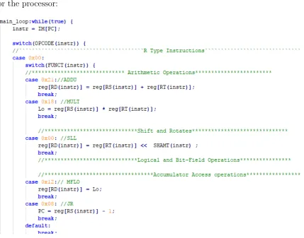
functionality occurs. Figure 3.2 displays a portion of an example architecture created

for the processor:

Figure 3.2: Portion of Example Processor Architecture

As is shown in Figure 3.2, case statements are used to switch between different

types of operations. Each operation is based on a MIPS instruction type. An

instruc-tion type is chosen based on an OPCODE and then an operainstruc-tion is chosen based

on the FUNCT of the instruction. Following this style allows a programmable

ver-sion of a MIPS architecture to be created. The shown architecture was designed for

a dot product application as the operations shown (and additional operations not

instructions ready to be chosen even if the application did not utilize the instructions

which leads to an excess of resource utilization. This methodology averts this by

using the process described.

The next step in stage 2 of the process shown in Figure 3.1 is to take the

architec-ture code, configured only with the required instructions, and use Vivado HLS [12] [13]

to generate Hardware Description Language (HDL) files. The designed architecture

code is used as a basis to create the datapath in HDL. During this process, directives

can also be applied to the architecture code. Directives are different characteristics

that are applied to program when being compiled into HDL such as pipelining,

regis-ter partitioning, etc. For our research, the code was pipelined. The HLS environment

generates HDL code specifying a datapath with the applied directives. The generated

HDL code is known as the Architecutre HDL, as shown in Figure 3.1.

The next step, which can be done in parallel to the HDL generation step, is to

use the created assembly source file from stage 1 of the process as the source for the

Assembler to generate the kernel binary files. Therefore, this step is the link between

stage 1 and stage 3. This is done by converting the assembly code to machine code.

Using the asm2mach tool in Eclipse [18] with the previously created .s file, .data and

.instr files are generated which represent the application in a machine data format.

These binary files are created so that the Architecture HDL can be applied to the

application code in a machine data format.

Once all of the necessary files are created to implement the processor and the

application, stages 1 and 2 of the process connect in stage 3 by creating a Xilinx

Integrated Synthesis Environment (ISE) Design [14] project which utilizes the

gen-erated Architecture HDL files and the kernel binary files to test the design through

simulations. In order to properly simulate the design, a testbench must be created

and utilized. This testbench would test the functionality of the algorithm, interact

CHAPTER 3. PROPOSED METHODOLOGY

the instruction and data files that were generated from the creation of the binary

files (based on the application source code). The testbench uses the .data and .instr

files to test the application using the processor files (datapath) from the minimalized

architecture. Thus, the application is tested on the pipelined processor. The design

is then simulated using tools such as ISim [11] or ModelSim [15]. Observing the

simulation allows performance determination of the application on the customized

processor. This process was used to verify the estimations of the applications that

3.3

Graph-based Approach

The basis of this research is to see how well we can estimate the performance of

the applications by first creating a graph of the application based on its C code

and observing the schedule. This type of graph is comparable to what is known as

a dataflow graph. A dataflow graph is a binary tree style graph that represents the

application by the operations that are performed. This graph shows the dependencies

that exist between the operations as it relates to the application as well as the relation

to the pipeline(s) for the architecture which is used as a basis for creating such a graph.

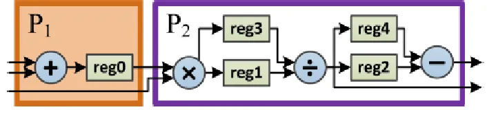
Figure 3.3 shows an example pipelined architecture design:

Figure 3.3: Example Pipelined Architecture [5]

This design, as shown, is comprised of two pipelines. An example dataflow graph

is then created for the application and shown in terms of uses for each pipeline:

Figure 3.4: Example Dataflow Graph [5]

CHAPTER 3. PROPOSED METHODOLOGY

uses for the first pipeline and the second pipeline. A pipeline’s use extends through

the levels (L) of the graph. This particular graph is shown to have 4 levels, marked L1

through L4. This is best demonstrated by observing the purple boxes in both Figures

3.3 and 3.4. As is shown in Figure 3.3, the purple box is indicative of the second

pipeline which contains a multiply operation, a division operation, and a subtraction

operation. Following the flow shown in Figure 3.3, it can be seen that the subtraction

operation is not mandatory and can be skipped if so desired. Observing Figure 3.4,

each purple box shows a use of pipeline 2. As is seen, a single use of the pipeline will

extend through the levels of the graph because operations still remain (that can be

used) pertaining to that pipeline. For this reason, a multiply operation in L2 and a

division operation in L3 are part of the same pipeline use. But, any other multiply

operations in L2 would require another use of the pipeline because the multiply

op-eration in the initial use of the pipeline already occurred. The problem that can be

encountered with this dataflow graph approach is that for large applications,

schedul-ing the graph can consume a lot of memory. This is because of the dependencies

that exist within the graph and that would have to be maintained in relation to the

pipeline. For this reason, a reduced graph approach had been previously researched.

From the dataflow graph in Figure 3.4, a reduced graph can be created:

based on the operations per level. A reduced graph is based on a dataflow graph where

only the number of each type of operation is stated for each level of the graph and from

which a schedule can be determined. The reduced graph essentially tallies the number

of times each operation is used in each level of the full graph. For example, as shown

in Figure 3.5, L2 has two addition operations and three multiplication operations.

In the reduced graph, only the number of uses for each operation is shown so L2

is shown to use two ’+’ operations, three ’x’ operations, and no other operations.

This reduced graph helps to condense the full graph into a format which is easier

to understand and from which further actions can be taken. As stated previously,

the benefits the reduced graph provides revolve around memory footprints. Storing

a large dataflow graph would require the use of an adjacency list as compared to

a small array for the reduced graph. Though the benefits might not be noticed in

the situation of having a small dataset, larger datasets would realize the benefit this

approach brings. For example, the dataflow graph for matrix-matrix multiplication

of 8192x8192 sized matrices would result in almost 8TB of required storage. If the

reduced graph approach is used, the information can be demonstrated by using a

13x2 array resulting in only 104 bytes of storage needed [5]. The tradeoff for this

approach is that dependencies for the graph will be lost, but for larger datasets, the

tradeoff is well worth it.

Regarding the schedules of the graphs, a schedule obtained from the dataflow

graph would result in what is known as the execution schedule. A schedule based

on the reduced graph would result in what is known as the reduced schedule. An

CHAPTER 3. PROPOSED METHODOLOGY

Figure 3.6: Example Pipelined Architecture Reduced Schedule [5]

As is shown in Figure 3.6, the number of operations related to each type of

oper-ation are scheduled through the levels of the graph. This is done by scheduling one

operation of each type per level if that operation was used, until there longer remains

any number of operations for that type. Understandably, this would result in much

lower memory consumption because the scheduling of the operations becomes easier

and doesn’t have to rely on any other operation type.

For our research, we are more concerned about the execution schedule. The

exe-cution schedule will depict the actual exeexe-cution of the application as it relates to the

original architecture. Therefore, it can be indicative of the performance on the actual

platform. The execution schedule is not necessarily the most optimal schedule for the

application, but it depicts how the application will actually run based on the pipeline

applied to the architecture. The optimal schedule results from the reduced schedule

which would also require an update to the architecture of the platform. Using this

Figure 3.7: Example Pipelined Architecture Execution Schedule (E - Epoch) [5]

Observing the execution schedule shows that the nodes shown in Figure 3.7 and

the reduced graph relate to the schedule after the structure of the pipeline is taken

into account. The addition operation in L1 is scheduled first. Using the pipeline,

we know that the multiplication operation would be the next operation scheduled

because it utilizes data from the previous operations. Since that is the case, all of the

multiplication operations in L2 will be scheduled after which the remaining additions

can be scheduled because there is no longer a need for the initial addition operation

to continue execution. The rest of the operations carry out in the same way but no

delays occur because the values of each remaining operation requires are available

from the previous parts in the pipeline.

An ”epoch” is the set of nodes that are executed concurrently. The ”span” is the

length of the schedule (or the number of epochs that it takes to complete the task,

i.e. to schedule all nodes onto the pipeline) and it is the aspect of this methodology

that we are interested in because it can be used to estimate the performance of the

application. Our hypothesis is that the span of the graph is directly proportional to

the execution time of the graph. By assigning a cycle count to each epoch, we are

CHAPTER 3. PROPOSED METHODOLOGY

To summarize, as mentioned before, our research uses a customized ISA processor

which has been pipelined using the process described in section 3.2. Certain

ap-plications are examined and the graphs of the apap-plications are determined. Those

graphs are then scheduled onto the customized ISA pipelined processor. The span is

also determined so that performance can be estimated and is then compared to the

3.4

Applications

In this work, the customized ISA soft processors were designed as described in section

3.2 and two different types of experiments were used to estimate performance of the

software implementations: varied-input size and varied-implementation. For this

pur-pose, two applications were examined: dot product and 128bit Advanced Encryption

Standard (AES). Two separate processors were implemented, one for the dot product

application, and one for the AES applications.

The dot product application represents the varied-input size experiment where

the size of the input vectors can be altered to observe changes in performance. As it

pertains to this application, the processor remained the same regardless of the size of

the input vectors.

The AES applications represent a varied-implementation experiment. Both the

standard 128bit AES implementation and the 128bit AES using TBox implementation

were examined. AES using TBox uses more Lookup Tables (LUTs) in the application

code to replace operations occurring in the rounds. By doing so, there are less

com-putations performed and the implementation is known to have better performance

than the standard approach. This aspect made AES and AES using TBox a good

experiment as the methodology can be tested on two different implementations of the

same algorithm. With regard to the AES applications, again the processor remained

the same regardless of the implementation. This was done to establish a level of

con-sistency when testing the methodology and because both applications use the same

type of instructions but vary in usage rate. The processors are fully sequential and

CHAPTER 3. PROPOSED METHODOLOGY

3.4.1 Dot Product

The dot product application followed the standard algebraic definition of a dot

prod-uct:

n

X

i=1

aibi =a1b1+a2b2+...+anbn (3.1)

This was a simple implementation using vectors as the data structure for holding

the input values. By varying the size of the vectors and increasing the number of

elements in the vectors, different test cases were created for this type of experiment.

Any size vector could be used and to better analyze the performance estimation,

many different vector sizes were tested. As had been stated previously, the flexibility

provided by the dot product algorithm allows this varied-input size experiment to be

conducted.

3.4.2 AES

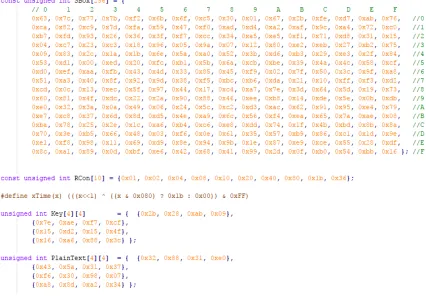
128bit AES is is an encryption algorithm standing for Advanced Encryption Standard,

otherwise known as the Rijindael algorithm [6]. The algorithm consists of various

stages of operations that are performed for numerous rounds. The stages are outlined

in Figure 4.4. The basic concept is that a 4x4 block of plain text would undergo several

Figure 3.8: 128bit AES Standard Implementation Initialization

The first stage of the encryption is to copy the encryption key and then perform a

key expansion. Key expansion produces different sub-keys and each sub-key pertains

to a different round of the algorithm. In order to specifically perform 128bit

encryp-tion, 10 rounds are used for the majority of the program. In comparison, 192bit AES

required 12 rounds and 256bit AES requires 14 rounds. So, specifically for 128bit

AES, a separate round key is required for each round, plus one more key (hence the

initial key copy). After expanding the key, the PlainText is copied to reserve the

original version. To finish up the initial round, an AddRoundKey stage is performed.

In this stage, a bitwise XOR is performed between the state array and the round key.

The stated actions are all a part of the initial round. For the first 9 rounds, five

differ-ent actions are performed. The first action is the SubBytes operation. This is where

CHAPTER 3. PROPOSED METHODOLOGY

state. The next action is the ShiftRows operation where the last three rows of the

state are shifted a number of times. The following step is the MixColumns operation.

This operation performs a matrix multiplication between a constant matrix and each

column of the state to produce resulting columns states, providing diffusion to the

cipher. The next step is to perform a memory copy so that the state can be preserved.

The last operation of the round is to perform another AddRoundKey operation with

the round sub-key. For round 10, the same operations shown in the first 9 rounds are

followed except for the MixColumns operation. Performing these 10 rounds provides

a 4x4 encrypted block of the original PlainText.

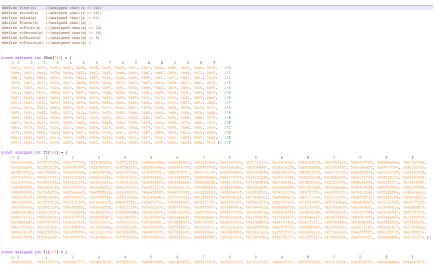
The TBox approach uses 4 more lookup tables filled with pre-determined values.

These values are the result of in-between operations during the stages of AES. By

having these values pre-determined and listed in lookup tables, those calculations can

be skipped during the actual encryption. Instead of performing these calculations,

the lookup table is indexed based on the state array. This helps to increase the

performance of the algorithm since fewer calculations are needed during the rounds,

thus improving the the overall performance of the actual encryption. This method

allows a differentiation to occur between the standard encryption method and the

TBox method. Therefore, it allows an experiment to take place since an increase

in performance is known to exist due to the dip in operations required to perform

the encryption. This method was also chosen because it is easy to implement once

the standard AES has already been implemented. The goal of this experiment also

does not revolve around how the performance is affected by a change in given

in-put (PlainText). Figure 3.9 shows the partial initialization of the AES with TBox

CHAPTER 3. PROPOSED METHODOLOGY

3.4.3 Instructions

As was stated previously, different MIPS instructions are used to implement the

architecture of the processors for both applications. Table 3.1 shows the different

instructions used and which application used which instructions:

MIPS Instruction Usage per Application Instruction Dot Product AES

ADDU Y Y

MULT Y N

SLL Y Y

MFLO Y N

XOR N Y

JR Y Y

ADDIU Y Y

ORI Y Y

ANDI N Y

LUI N Y

LW Y Y

SW Y Y

SLTIU N Y

SLTI Y N

BEQ N Y

BNE Y Y

BGEZ Y Y

3.5

Preliminary Analysis

Before progressing with applying the graph-based methodology to the applications

described, a determination had to be made as to whether this approach can be viable

or not. In order to do this, the implementation flow described in section 3.2 was

applied to the dot product application. So this means that the dot product application

(initially using a small input vector size of 3) was implemented on a customized ISA

processor. The simulation of the ISE project (based on the HDL of the customized

dot product architecture and kernel binary files) was then observed. The goal of this

initial analysis was to determine if a pattern could be found in the output stream of the

simulation. Outputs appeared in the output stream after the instructions/operations

related to that output had been processed/performed. Therefore, it is indicative

of the actions/stages that take place during the execution of the application. If a

pattern could be found by observing the execution schedule of the application on

the customized processor, then the belief was that a graph-based methodology would

be a usable approach because an observable pattern could likely be put into a graph

format. Observing the simulation and how the instructions/operations were processed

and then output for a small input size would enable any pattern observed to be

applied to larger input size vector dot product application, thus allowing for a form

of estimation to take place. The number of cycles that were observed for each part of

the pattern pertain to how long the current action (referred to as stage) of the output

was shown in the output stream while the next action/stage of the application was

processed. This was done because the output stream is indicative of the the overall

CHAPTER 3. PROPOSED METHODOLOGY

Figure 3.10: Sim. Observation for Dot Product with Input Vectors [1, 3, 5] and [4, 2, 1] Iteration - Current iteration of the main ’for’ loop in the application

Input- Current element being processed from the input vectors

Mathematical Output- Output of dot product between current elements of input vectors

When observing the simulation for a dot product application with an input vector

size of 3, the pattern that was noticed in the output was that essentially four rounds

take place, as shown in Figure 3.10. A round is a set of actions/stages that take

place related to each iteration in the main ’for’ loop in the dot product application.

In the first round (called round zero), the current iteration of the main ’for’ loop is

displayed, followed by the first element of the first input vector. The current iteration

for round zero is then shown again followed by the first element of the second input

vector. The current mathematical output is then displayed in the output stream.

The mathematical output is the actual dot product mathematical operation that

takes place. So, for this specific application it would be [sum + (current element

of first input vector * current element of second input vector)]. During round zero,

this is still 0 because the operation has not been completed yet since the inputs were

only just processed. The current iteration for round zero is shown one more time.

The same process then happens for 2 more consecutive rounds except that when the

current mathematical output is displayed, it pertains to the previous round. So in

round one, the mathematical output related to the inputs processed in round zero is

shown. In round two, the mathematical output based on the inputs and mathematical

processed in round zero are 1 and 4, the mathematical output of round zero will be

0 because the computation is still not complete yet. If the inputs processed in round

one are 3 and 2, the the mathematical output of round one is 4 because it pertains to

the previous round (since the calculation has now been completed), thus performing

the operation 0 + (1 * 4). If the inputs processed in round two are 5 and 1, then the

mathematical output of round two is 10 because it builds off of the previous round,

thus performing the operation 4 + (3 * 2). The last round only contains two actions,

displaying the iteration and then displaying the final mathematical output. For the

described example that would be 15 because the operation performed is 10 + (5 *

1). Essentially this means there is a one round lag in displaying the output. The

other difference between the first round (round zero) and all following rounds, that

are not the last round, is that the first time the current iteration is shown, in rounds

one and two, it takes less cycles than in round zero. This is why in Figure 3.10 round

zero takes more cycles than rounds one and two. This is attributed to a form of

initialization in round zero. Another observation that was noted was the amount of

time taken for the initialization of the processor itself, before the stages of the rounds

even begin to be displayed in the output stream. This was called the initiation period.

The same was observed for the end of the application to determine how many cycles

were taken to clear the streams and completely finish execution of the application.

The ending stage was known as Finalization and was observed to always be 10 clock

cycles.

After performing these observations for an input vector size of 3, the same

ap-proach was followed for larger input size vectors. The same apap-proach was taken for

input vector sizes of 8, 10, and 15. Again, this was done to see if the same pattern in

the rounds existed. It was found that the pattern does exist. The first round (round

zero) always follows the pattern described and each subsequent round that is not the

CHAPTER 3. PROPOSED METHODOLOGY

Then each final round follows the same pattern.

The aspect that changes is the execution time of the initiation of the application

on the processor. With an increase in the number of elements, the initiation cycles

increase. This was expected, but the question was if it is also something that follows

a pattern. It was determined that it does follow a pattern. A base 14 clock cycles

always exist in the initiation period followed by 8 clock cycles for each additional

input element. So, a dot product application with an input vector size of 3 would

have 6 elements. Therefore, its initiation period (as shown in Figure 3.10) would be

14 + (6 * 8) = 62 cycles. Another example is an input vector size of 8 would have

16 elements. Therefore, its initiation period would be 14 + (16 * 8) = 142 clock

cycles. Observing all of these patterns for varying input sizes allowed us to be able

to accurately estimate the performance of the dot product application for any given

input vector size with the estimation always being 100%.

When conducting this analysis, it was believed that such a situation would allow

a graph to be constructed since a pattern existed. Upon further examination, this

was not necessarily the case. It is true that fully accurate estimations were made,

but they did not fit well in a graph structure. With a constantly varying initiation

period and an extra round taken to display the final output, putting the pattern into

a general form graph would prove to be out of scope of what the basis of this research

is. To reiterate, the basis of the graph-based approach is to be able to observe the

application from a high-level and derive a graph from it. Things such as displaying the

current iteration multiple times and a constantly changing initiation period would not

make this approach ideal. The desired approach was to schedule the graph after it was

created and then apply a value to each epoch to be able to estimate the performance.

Doing so using the pattern determination approach would be cumbersome because

the goal is to be able to obtain an estimation which is independent of the hardware

the assembly for the specific hardware platform. In addition, the clock cycle count

changes per stage and thus a more general form of applying a clock cycle count to

each epoch was also desired, inherently making the estimation less accurate.

The other aspect to consider is that this was done for a varied-input size approach.

If the pattern determination approach was followed and a graph was constructed, it

would be of little use for the varying implementation approach. This is considered

the trade-off of using the proposed graph-based approach. Even though we are able

to obtain exact estimations for any input size for the dot product application, that

approach deviates from the basis of this research. We needed a more general approach

that could be applied to different types of applications by observing them from a

high-level C code implementation. Taking the pattern detection route would also prove

to be much more time consuming when applied to an application such as AES than

the alternative graph-based approach that has been proposed. For this reason, this

approach was not used and the approach that was used is described in chapter 4.

Again, the trade-off for not having 100% accuracy but still having good estimations

(described in chapter 4) is being able to apply this approach to more applications,

being able to actually create a proper graph for the application, and reducing the

time and workload needed to achieve the estimation.

Another aspect that was involved in the preliminary analysis that was conducted

relates to the scheduling of the application. As was explained in section 3.3, both a

reduced schedule or an execution schedule can be created based on the graphs and

the pipeline. During the initial stages of the current research, it was believed that

the desired schedule was the reduced schedule. For this reason, a C++ program was

in development to be able to take any dataflow graph and schedule it in a reduced

schedule. After determining that the execution schedule was the desired and

appro-priate route to take, development on the previously described program was halted

CHAPTER 3. PROPOSED METHODOLOGY

graph and create the execution schdule based on the pipeline. This was then

deter-mined to not be needed because what was actually desired was the span of the graph.

So, a general program was written to be able to calculate the span of any dataflow

graph based on the approach described in chapter 4. This program was helpful to

3.6

Experimental Setup

The experimental setup was designed to be able to test both cases, varied-input

size and varied-implementation. As it pertains to varied-input size, the dot product

application was used and the input vector sizes were varied (2, 3, 5, 10, 15, 20, 50, 75,

100, 150). For each input size, the span of the graph was found and the performance

was estimated using characteristics of the pipeline. The implementation flow (Figure

3.1) was then followed for every input size to determine the actual performance of the

dot product application on the customized ISA processor. The true performance data

was gathered for each input size from the simulator, ISim, running the ISE design

project. The estimated performance was then compared to the actual performance

to determine how accurate of an estimation it was.

As it pertains to the varied-implementation test case, the graphs for AES and AES

using TBox were created and the performance was estimated using characteristics of

the AES pipeline. Both applications were then put through the implementation flow

to determine how long each actually takes on the customized ISA processor. The

actual, observed performance data was gathered for each application. After doing so,

the estimated performances were again compared to the actual performances to see

Chapter 4

Results

As was shown in section 3.3, this graph-based approach is capable of handling multiple

pipelines for a single application but that feature is not applicable to our

implemen-tation because for us there is only a single pipeline that is used for the application.

We are interested in how long the schedule of the graph will be which is known as the

span of the graph. After extracting the graph from a C description of the application,

we find the span of the graph, schedule the graph and determine a cycle count for

each epoch based on characteristics of the pipeline. In order to determine the span

of the graph, the number of uses for each pipeline is first taken at each level and the

maximum value amongst them is found. This is the epoch count as it relates to that

level of the graph. The span is simply the maximum of 1 and the epoch count for

each level. This is done in the case that the epochs required for a certain level is

zero. If this is the case, then 1 needs to be added to the span to account for pipeline

latency [5]. In order to visualize this, Figure 4.1 applies the stated method to the

Figure 4.1: Example of Span Determination

As is shown, the total span of the example graph comes out to be 6 cycles after

following the process motioned above. The first application this was applied to was

the dot product application. As the graphs can become large, this was initially applied

CHAPTER 4. RESULTS

4.1

Dot Product Results

Figure 4.2 shows the scheduled graph for a two vector, one element dot product

application.

Figure 4.2: Scheduled Graph for 2 vector, 1 element Dot Product Application

This graph was determined based on extracting steps out of the C code. Notice

that there is only one step being performed for each level of the graph of the

ap-plication. This is because, as mentioned previously, the processor being used is a

sequential processor and therefore only one action can be performed on each step of

the graph, which leads the graph shown to actually be the scheduled graph on the

customized ISA processor. Following the graph-based approach, this actually leads

one use of the pipeline and there is only one type of pipeline which is used for this

application. Increasing the input size by 1 increases the size of the graph by 10. This

trend will continue for all input sizes for the dot product and therefore it is easy to

predict how large the graph for any size input for dot product will be. This means

that the estimated span of the dot product graph can be easily known.

The next step is to determine how many cycles will each epoch take based on

characteristics of the application. For this, the number of cycles it took for major

types of instructions to get from the input of the pipeline to be shown in the output of

the pipeline is determined. This means, the number of cycles taken for an instruction

to begin in the pipeline and the result to show in the output of the pipeline was

observed.

In order to take this approach, the main types of instructions were examined as

determined by the C code of the application and the scheduled graph. An instruction

was classified as a main instruction if it is a defining operation in the application

(such as addition and multiplication for Dot Product) or an instruction needed for

the defining operation to be used (such as a memory access). For dot product, this

turns out to be a memory access, addition, and multiplication, which took 2 cycles,

10 cycles, and 14 cycles respectively. These cycle counts were determined by creating

targeted C code to be able to test the specific instruction, observing the simulation

of the pipeline using ISim and counting how many cycles it took for the instruction

to be able to display it’s action out of the pipeline. By taking the average of these

values and flooring (to avoid overestimation), we are left with an 8 cycle average.

This average is then applied to each epoch of the dot product graph to give us an

estimation of how long the program will take to process in the simulation. This

will vary as the input size increases/decreases. As an example, applying this cycle

count to a dot product application where each input vector is of size 2, the predicted

CHAPTER 4. RESULTS

that this research focuses on the fact that a cycle count can be applied to each epoch

to provide an estimation, the general focus is not on the approach taken to obtain

that cycle count. The approach described above is simply the route taken to obtain

4.1.1 Dot Product Results Analysis

In order to view the estimation of the Dot Product and the trend that occurs for

estimation of a varied-input size test case, a table and a plot were created. Table 4.1

shows the numerical results of the Pipelined Dot Product Performance Estimation:

Pipelined Dot Product Performance Estimation Input Size Estimated Cycles Real Cycles %Accuracy

2 160 244 65.57

3 240 336 71.43

5 400 520 76.92

10 800 980 81.63

15 1200 1440 83.33

20 1600 1900 84.21

50 4000 4660 85.84

75 6000 6960 86.21

100 8000 9260 86.39

150 12000 13860 86.58

Table 4.1: Performance Estimation of Pipelined Dot Product

The trend that is apparent in Table 4.1 is demonstrated in Figure 4.3. As can be

seen in Figure 4.3, as the size of the input increases for the dot product application,

the more accurate it becomes, eventually leveling off at around 87% accuracy of

estimation. Due to the trend of the graph, it can be assumed that at even larger

input sizes, the level of accuracy of estimation will be approximately 87%. For this

reason, larger sizes were not run, but the mathematical relationship in the results

shown in Table 4.1 was analyzed with an input size as large as 1500. The result

CHAPTER 4. RESULTS

Figure 4.3: Performance Estimation of Pipelined Dot Product

4.1.2 Dot Product Results Discussion

As it pertains to the varied-input size test case of the methodology, this method of

estimation is intended for larger data sizes and it is shown to be quite effective for

the Dot Product application. As can be shown in Figure 4.3, for larger data sizes,

the approach estimates with about 87% accuracy. The missing 13% in estimation is

attributed to aspects discussed in section 3.5. The goal of the research was to be able

to have an estimation approach that is independent of the hardware implementation.

An exact estimation can be obtained but the approach that would need to be taken

is not the basis of the research. The purpose of this type of estimation is to be able

to estimate from a much higher level, just by viewing C code and being able to create

a graph from it so that the approach used would be a general approach that could be

a constantly varying initiation period and displaying the current iteration multiple

times that take place in the actual simulation, as described in section 3.5. Because of

these aspects, the estimation will not be necessarily be near 100% accuracy. This is

the trade-off of being able to create a higher level graph and estimating from a more

coarse-grained view. Taking this into account, it was determined that the approach

CHAPTER 4. RESULTS

4.2

AES Results

The same process was applied to both the AES application and the AES with TBox

application. For the original AES implementation, the graph was simplified to what

is shown in Figure 4.4.

Figure 4.4: High Level Dataflow Graph of AES

Due to the length and depth of the AES application itself, Figure 4.4 is presented

to provide a higher level of view of how the AES application actually functions.

Breaking the graph down appropriately to match the level of depth of the dot

prod-uct graph gives a span of 10,242 which gives us 10,242 epochs. Again, the same

methodology is applied to the AES application that occurred for the Dot Product

application. The most prominent operations in the AES application were addition

instruction, observing the simulation of the pipeline using ISim and counting how

many cycles it took for the instruction to be able to display it’s action out of the

pipeline. Averaging these values and then flooring (to avoid overestimation) gives us

6 cycles. This value is then applied to each epoch to give us a total estimation cycle

count of 61,452 cycles.

Again, the same methodology was applied to AES with TBox. The graph for the

AES with TBox application was also presented with a higher level of view to show

how it actually functions.

Figure 4.5: High Level Dataflow Graph of AES with TBox

Figure 4.5 represents how the AES with TBox application operates. The

dif-ferences that can be observed between this implementation and the standard AES

implementation are that AES with TBox has a specific part just to perform TBox

operations. The SubBytes and ShiftRows operations are also combined into a single

operation rather than being separated. The largest difference is that the MixColumns

and MemCopy parts were no longer explicit operations in the rounds because of the

CHAPTER 4. RESULTS

graphs and doing so gives a span of 4,640 and 4,640 epochs to the graph. This is

significantly less than the original AES implementation which is what was expected

since using the TBox implementation cuts out a lot of operations/instructions that

the original implementation had to go through. The operations/instructions that are

not needed anymore are numerous memory accesses and xor operations that occurred

during multiple rounds. These values were replaced with just a reduced number of

memory accesses and xors because the of the LUTs. Again, the same methodology is

applied to the AES with TBox application that occurred for the Dot Product

appli-cation and the original AES implementation. The most prominent operations in the

AES application were addition (8 cycles), xor (8 cycles), ori (8 cycles), and a memory

access (2 cycles). These cycles counts were observed by creating targeted C code to

be able to test the specific instruction, observing the simulation of the pipeline using

ISim and counting how many cycles it took for the instruction to be able to display

its action out of the pipeline. Averaging these values and then flooring (to avoid

overestimation) gives us 6 cycles. This value being so similar to the original AES

implementation is what was expected since the AES with TBox actually utilized the

same architecture as the original AES implementation. This was done partly to try

and establish a level of consistency and truly show a varied-implementation test case.

This value is then applied to each epoch to give us a total estimation cycle count of

4.2.1 AES Results Analysis

After applying the discussed methodology to the different implementations under

examination, results ranged from 75% accuracy to 89% accuracy. In order to view

the estimation of the AES implementations and the trend that occurs for estimation

of a varied-implementation test case, a table and a plot were created. Table 4.2 shows

the numerical results of the Pipelined AES Performance Estimation:

Pipelined AES Performance Estimation

Implementation Estimated Cycles Real Cycles %Accuracy

Standard AES 61452 81723 75.195

AES using TBox 27840 31383 88.71

Table 4.2: Performance Estimation of Pipelined AES

The data that is shown in Table 4.2 is demonstrated in Figure 4.6. As can be

seen in Figure 4.6 and Table 4.2, the original AES application took 81,723 cycles and

the methodology provided an estimate of 61,452 cycles. Therefore, the methodology

used was able to estimate the performance of the AES application with approximately

75% accuracy. Figure 4.6 also shows the results of estimation for the AES with TBox

implementation. As is shown, the AES with TBox application took 31,383 cycles while

the methodology provided an estimate of 27,840 cycles. Therefore the methodology

used was able to estimate the performance of the application with approximately 89%

accuracy. In the experiment, one clock cycle was 10ns following what is observed for