Electrical Impedance Based Spectroscopy and Tomography Techniques for Obesity and Heart Diseases

(1)

Electrical Impedance Based Spectroscopy and

Tomography Techniques for Obesity and

Heart Diseases

Thesis by

Shell Xiaoxiao Zhang

In Partial Fulfillment of the Requirements for the degree of

Doctor of PhiΦlosophy

CALIFORNIA INSTITUTE OF TECHNOLOGY Pasadena, California

2017

(2)

 2016

Shell Xiaoxiao Zhang

(3)

(4)

(5)

ACKNOWLEDGEMENTS

I would like to express my special appreciation and thanks to my advisor Professor Yu-Chong Tai. Professor Tai has been a tremendous mentor for the past five years for me. He has taught me how to conduct research in world class, and perhaps even more importantly, how to think deeply and critically about matters in hand. Professor Tai's never-ending supply of fresh ideas and enthusiasm for research has been a source of inspiration for my own work. I am extremely fortunate to have conducted my graduate work under his guidance.

I would like to thank Professor Hsiai for his guidance and invaluable effort in our collaboration. He was the steering wheel for our projects, without Professor Hsiai's efforts both the EIS and EIT project would not have reached their milestones.

I would like to express my gratitude towards my colleagues Dr. Luo Yuan, Dr. Lei Xu, and Dr. Ming Xu. My work would never have been successful without their dedication and tremendous effort to our project. I was very fortunate to have such capable and wonderful colleagues to be able to conduct and finish all aspects of both EIS and EIT projects. I would also like to acknowledge all members of Professor Tai's lab, who have helped me along the way, and have been inspirations and sounding boards of my

research.

(6)

(7)

ABSTRACT

Despite advances in diagnosis and therapy, atherosclerotic cardiovascular disease remains the leading cause of morbidity and mortality. Predicting metabolically active atherosclerotic lesions has remained an unmet clinical need. Specially, atherosclerotic plaques that are prone to rupture are of extremely high-risk and can cause detrimental heart attacks and/or strokes, leading to sudden death. It has been shown that atheroscleroses is correlated to the level of obesity of an individual [1] Usually in clinical practice, the doctor will assess a patient's “risk factor” based on his or her Body Mass Index (BMS), and measurement of the waist circumference. Meanwhile the level of fatty droplet deposits in the liver is an important bio-marker to assess the patient's risk factor, however the patient will need to undergo radiation imaging such as CT scan or MRI scan.

(8)

(9)

PUBLISHED CONTENT AND CONTRIBUTIONS

Packard, R. R. S., Zhang, X., Luo, Y., Ma, T., Jen, N., Ma, J., Hsiai, T. K. (2016). Two-Point Stretchable Electrode Array for Endoluminal Electrochemical Impedance

Spectroscopy Measurements of Lipid-Laden Atherosclerotic Plaques. Ann Biomed Eng, 44(9), 2695–2706. doi:10.1007/s10439-016-1559-9

Shell (Xiaoxiao) participated in the conception of the project, designed and fabricated the device, participated in the data collection during experiment, prepared the data, and participated in the writing of the manuscript.

Packard, Rene., Zhang, Xiaoxiao., Luo, Yuan., et al., “The next generation of stretchable sensors for intravascular electrochemical impedance spectroscopy of varying levels of lipid burden and atherosclerosis,” American Heart Association (AHA) Health Tech, Session Title” Emerging Technologies (November 2015), vol. 132 no. Suppl 3 A18004. doi: 10.1016/j.bios.2013.11.059

Shell participated in the conception of the project, designed and fabricated the device, participated in the data collection during experiment, prepared the data, and participated in the writing of the manuscript.

(10)

Cao, Hung, Fei Yu, Yu Zhao, Xiaoxiao Zhang, Joyce Tai, et al. "Wearable multi-channel microelectrode membranes for elucidating electrophysiological phenotypes of injured myocardium." Integrative Biology 6, no. 8 (2014): 789-795. doi:10.1039/c4ib00052h

Zhang, Xiaoxiao, Beebe Tyler, et al. “Wearable flexible micro electrode for adult zebrafish long term ecg monitoring,” In Micro Electro Mechanical Systems (MEMS), 2015 IEEE 28th_{International Conference. doi:10.1109/memsys.2015.7051051}

Zhang, Xiaoxiao, Joyce Tai, Jungwook Park, and Yu-Chong Tai. "Flexible MEA for adult zebrafish ECG recording covering both ventricle and atrium." In Micro Electro Mechanical Systems (MEMS), 2014 IEEE 27th International Conference on pp. 841-844. IEEE, 2014. doi:10.1109/memsys.2014.6765772

(11)

device, participated in the data collection during experiment, prepared the data, and participated in the writing of the manuscript.

Zhao, Yu, Fei Yu, Hung Cao, Honglong Chang, Xiaoxiao Zhang, Tzung K. Hsiai, and Yu-Chong Tai. "A wearable percutaneous implant for long term zebrafish epicardial ECG recording." In Solid-State Sensors, Actuators and Microsystems (TRANSDUCERS & EUROSENSORS XXVII), 2013 Transducers & Eurosensors XXVII: The 17th International Conference on, pp. 756-759. IEEE, 2013. doi:10.1109/transducers.2013.6626876

(12)

(13)

LIST OF FIGURES AND TABLES

Number Page

1. Fig. 1.3.1.1.1: Histology of a lipid-rich “vulnerable” coronary plaque. Pg 8

2. Fig. 1.3.1.1.2: Morphological traits associated with vulnerable plaques Pg 8

3. Table. 1.3.1.2.1: Comparison of Noninvasive and Invasive imaging modalities for detection of individual characteristics of vulnerable plaques... Pg 11

4. Fig. 2.1.1: A diagram illustrating how the phosphoglyceride (or phospholipid) molecules behave in water... Pg 20

5. Fig. 2.1.2: The structure of a cell membrane with one ion channel... Pg 20

6. Fig. 2.3.1: Diagram of equivalent circuit of a cell model... ….. Pg 27

7. Fig. 2.3.2: Permittivity variation of a tissue as a function of frequency... Pg 28

8. Fig. 3.1: Energy vs. frequency band for Electromagnetic waves... Pg 31

9. Fig 3.2.1: volume conductor with four electrode...Pg 35

(19)

11. Fig. 3.4.2: Randle's circuit... Pg 41

12. Fig. 3.4.3: Electrode-electrolyte equivalent circuit w/ small perturbation... Pg 41

13. Fig. 3.5.3: Effect of Structural Design of Silver/Silver Chloride Electrodes on Stability and Response Time ... Pg 43

14. Fig. 3.5.1.: Simulated amplitude Bode plot (up) and phase Bode plot (down) based on Randle's circuit in Fig. 3.4.2... Pg 45

15. Fig. 3.5.2: Simulated Nyquist plot of a of an ideal Randle's circuit based on Randle's circuit in Fig. 3.4.2...…... Pg 46

16. Fig. 3.5.1: tissue and electrode model for EIS measurement... Pg 47

17. Fig. 3.5.2: equivalent circuit of tissue and electrode model... Pg 48

18. Fig. 3.5.3: Impedance Bode-plot on log-log scale showing three corners.... Pg 49

19. Fig 4.1.1: System diagram of the Labview Based system...Pg 51

20. Fig 4.1.2: Pre-amp circuit diagram... Pg 52

(20)

22. Fig 4.1.4: Swisstom noise performance over 10 consecutive frames. LabView noise plot...Pg 54

23. Figure 5.1.1: (a): meshed artery segment with lesion... Pg 72

24. Figure 5.1.2: sensitivity field of different lengths …...Pg 74

25. Figure 5.2.1: (a) Design diagram of the Parylene-C electrode design...Pg 75

26. Figure 5.2.2: Finished integrated catheter device...Pg 76

27. Figure 5.3.1.1: Bottom: Parylene-C based micro electrode array. …...Pg 77

28. Figure 5.3.1.2: (a): ex-vivo mouse aorta EIS measurement setup. …... Pg 78

29. Figure 5.3.1.3: Left: Impedance amplitude and phase curves of lean muscle. Right: Impedance amplitude and phase curves of fat... Pg 79

30. Figure 5.3.1.4: Impedance modulus of sample I, II and III mice aortas... Pg 79

31. Figure 5.3.2.1: Finished integrated catheter device... ....Pg 82

(21)

33.

34. Figure 5.3.2.3: EIS results from different sites showing the impedance (top) and phase (bottom) differences between plaques of conditions from control (i.e., no plaque) to severe plaque...Pg 85

35. Fig 6.1.1 Inward imaging and outward imagingIn contrast to inward imaging, as a new imaging modality, we have developed “outward imaging”. …... Pg 88

36. Fig 6.2.1: Spread vs. number of electrodes. Spread is defined by the area of the reconstructed image divided by the area of the real object….. Pg 89

37. Fig 6.2.1: Reconstructed image of same 1mm diameter object placed at different distances away from the probe

edge... Pg 90

38. Fig 6.2.2: 100um – 2mm distances (first row of Fig 6.2.1) after 10% threshold crop, we define these to be the constructed object

size... Pg 90

(22)

40. Fig 6.2.4: reconstructed image of radius r at distance 100um from the probe edge...

Pg 92

41. Fig 6.2.5: 10% threshold cropped images from Fig 6.2.4, used to define the reconstructed image area and

size...Pg 93

42. Fig 6.2.6: Left: resolution of the reconstructed image with radius r at distance 100um to probe edge. Right spread of the reconstructed image with radius r at distance 100um to probe edge. Distance and object size...Pg 94

43. Fig 6.2.7 Combined result of varied radius vs. varied distance...Pg 95

44. Fig 6.2.8: Left: resolution vs. distance (blue object r = 0.5mm, red r = 2mm, green r = 4mm) Right: spread vs. distance (blue object r = 0.5mm, red r = 2mm, green r =

4mm)... Pg 95

45. Table 6.3.1: Conductivity values used in FEM simulation...Pg 97

(23)

47. Fig 6.4.1: Top left: electrode in saline. Top right: electrode zoom-in view. Middle row: “pen in saline” experiment setup. Bottom row: reconstructed images corresponding to pen location... Pg 100

48. Fig 6.4.2: (a) shows the EIT imaging results with the swine aorta sample and subcutaneous fat mimicking plaques through implementing a one-step fast algorithm... Pg 101

49. Fig 6.4.3: (a) red-blue scale reconstructed image with ex-vivo aorta

tissue... Pg 102

50. Fig. 6.4.4: phantom tank with 1/8 normal saline conductivity agar gel and ¼ normal saline background. …... Pg 118

51. Fig. 6.4.5: Difference imaging reconstruction …... Pg 119

52. Fig. 6.4.6: Absolute imaging reconstruction. The scale bar shows correct conductivity reading. …... Pg 119

53. Fig. 7.1.1: relative position of liver inside the human body... Pg 123

(24)

55. Fig. 7.1.3: electrode placement on human thorax... Pg 124

56. Table 7.2.1: conductivity major abdominal tissues from literature Pg 125

57. Fig 7.2.2: The effect of temperature on the electrical impedance spectra of (a) 100% liver and (b) 100% fat... ... Pg 126

58. Fig. 7.3.1: Left: FEM model used to generate voltage data. Right: Conductivity of each organ at 50Khz and

250Khz. ... Pg 127

59. Fig. 7.3.2: From left to right: 100% liver conductivity (healthy), 95% conductivity, 90% conductivity, 80% conductivity, and 70%

conductivity... Pg 128

60. Fig 7.3.3: Reconstructed “effective” conductivity in the liver region vs. the modeled liver conductivity plot... Pg 129

61. Fig 7.3.4: Left: FEM model used to generate voltage data. Right: Reconstructed image with 1% added random

(25)

62. Fig. 7.3.5: Left: FEM model (b) reconstructed image with inaccurate thorax geometry ... Pg 130

63. Fig. 7.3.6: Left: FEM model used for simulation study based on the CT scan. Right: CT scan image (mirrored)...

Pg 131

64. Fig. 7.3.7: (a) FEM model to generate voltage data (b) nconstrained higher order solver (c) smoothness constrain with a priori matrix in the liver region (d) smoothness constrain with a priori matrix in the liver region with shape

error... Pg 134

65. Fig. 7.4.1: Left: tank setup with 32 stainless steel

electrodes... Pg 140

66. Fig. 7.4.2. (a)(b)sensitivity field of adjacent injection pattern (c)(d) sensitivity field of opposite injection

(26)

67. Fig. 7.4.3 current lines near electrode with different contact impedance values from z=0.01 Ohm to z = 10Ohm. …... Pg 146

68. Fig. 7.4.4: Top: electrode pair contact impedance in series with saline. Bottom: Calculated contact impedance for each electrode. The last impedance is the resistance of

saline... Pg 148

69. Fig. 7.4.5: Left: reconstructed image with no contact impedance. Right:

reconstructed image with calculated contact impedance incorporated... Pg 148

70. Fig. 7.5.1: Impedance modulus (left) and phase angle (right) EIS with two

electrode method... Pg 150

71. Fig. 7.5.2: Agar gel mimicing subcutaneous fat in saline. Left: experimental setup. Right: Reconstructed image... Pg 150

72. Fig. 7.5.3: Subcutaneous fat experiment with pork fat in saline. Left: experimental setup. Right: Reconstructed image... Pg 151

73. Fig. 7.5.4: Liver experiment with pork liver. Left: experimental setup... Pg 122

(27)

75. Fig. 7.6.2: Left: experiment setup. Right: Reconstructed image with location difference data. ... Pg 154

76. Fig. 7.6.3: Left: two male test subjects with electrode belt position shown. Right: Reconstructed images correspondingly... ...Pg 155

(28)

(29)

C h a p t e r 1

INTRODUCTION

1.1 Bio-electricity in the human body

An important area of research concerns itself with the theoretical, modeling, and experimental results of current flow through and on the boundary of human tissue. Current flow within tissue is the result of electric potential gradients as part of internal biological functions as observed in cardiomyocytes and neurons. This line of research started in 1876 when Luigi Galvani began investigating the effect of current flow through the legs of frogs. Today cable theory with its mathematical derivatives provides a solid model for understanding neuronal electronic potentials.

(30)

resistivity contrast (up to about 200:1) between a wide range of tissue types in the human body (Geddes and Baker, 1967). It is this characteristic of tissue that has been utilized to differentiate between tissue and reconstruct spatial impedence maps of solid bodies. These impedence maps are calculated as an inverse problem using Laplace's equation. This way to visualize the human body is commonly known as electrical impedence tomography. EIT adds a soft field imaging modality to the repertoire of hard field imaging techniques in prevalence today.

1.2 Bio-impedance based diagnosis

Let us use the term EI imaging as an umbrella for various bio-impedance based imaging modalities which include EIS electrical impedance spectroscopy, EIT electrical impedance tomography, EFT electrical field tomography, MREIT magnetic resonance electrical impedance tomography, and MIT magnetic induction tomography.

Electrical Impedance Spectroscopy (EIS), This modality measures the impedance of a solid body over a range of frequencies, and therefore the frequency response of the body. The properties that can be resolved include the energy storage and dissipation property. Data from EIS is often represented as a Nyquist plot.

(31)

between normal and suspected abnormal tissue within the same organ (multifrequency-EIT).

Electric Field Tomography (EFT), is an imaging modality which enables contact-less sensing of spatial impedance maps in solid bodies. The body is probed by alternating quasistatic electric fields, with wavelengths much longer then the object of interest. Free charge carriers in the solid body can not redistribute immediately to compensate for changes in the external field producing a weak secondary field (Maxwell-Wagner relaxation) This weak secondary field depends on the conductivity, permittivity, geometry, and frequency of active current.

Magnetic Resonance Electrical impedance Tomography (MREIT), Is a dual imaging modality that utilizes the internal data of magnetic flux density in addition to the boundary current-voltage measurements to stitch together three-dimensional maps of conductivity and current density distributions.

Magnetic induction tomography (MIT) is an imaging modality used to image electromagnetic properties of an object by using the eddy current effect.

(32)

or Positron Emission Tomography PET. The size, weight and complexity of the probing apparatus and processing hardware is also greatly reduced with EIT.

(33)

Because electric properties of tissues are correlated with cell fluids, membranes, cell structure, any change to the measure of electrical scalar potential distribution and current flow through the body is a change in impedance due to a pathology or biological function change in the body. A transient decrease of cell membrane resistance during activity was proven by the experiments of Cole and Curtis [4]. Weinhold et al. [5] have used thoracic electrical impedance measures for early diagnosis of organ rejection in transplant recipients. Differentiation of tissue has been long researched but has not found its way into wide clinical adoption and points to an under-served opportunity.

1.3 Applications in this thesis

(34)

For the vulnerable plaques that can lead to sudden rupture, the ability to distinguish them at an early stage remains largely lacking. Therefore it is of great clinical interest to find improved diagnostic techniques to identify and localize such vulnerable plaques. Meanwhile, lipid has significantly lower electrical impedance than the rest of the vessel tissues in certain frequency bands [2]. In this thesis we explore spectroscopic and tomograφc methods to characterize such plaques. In addition, with the Electrical Impedance Tomography method we will propose a novel method to detect fatty liver in an early stage with non-radiating and non-invasive manner.

1.3.1 Endoluminal Vulnerable Plaque Detection

1.3.1.1 Introduction to the Disease

Although formation of atheromatous plaque has been well understood and lesion types characterized, the concept of the “vulnerable” plaque is a novel one. [6] The term vulnerable plaque refers to a subgroup of often modestly stenotic plaques yet prone to rupture. The ruptured plaque often results in acute coronary syndromes, and sudden cardiac death. The lack of prior symptoms make this disease especially dangerous.

(35)

Despite the on-going research effort and the progress that has been made, however, the exact factors that determine the fate of a plaque rupture are still unknown to-date.

[image:35.612.166.485.535.738.2]

There are currently several diagnostic tools that attempt to diagnose vulnerable plaques based on the above mentioned common characteristics. In the following section a brief overview of the state of the art diagnostic tools are provided.

(36)

Fig. 1.3.1.1.2: Typical morphological traits associated with vulnerable plaques

1.3.1.2 State of the Art Diagnostic Tools and Limitations

In recent years, cardiovascular research has sought potential strategies for detecting high-risk plaques before their disruption. These potentially powerful techniques are aimed at identification of populations at risk and plaque monitoring and might eventually guide targeted therapy.

Angioscopy: Angioscopy is the “gold stand” of characterizing the blockage of atherosclerosis. However since the vulnerable plaque is not charactered by its blockage of the lumen but rather most has an outward remodeling (meaning they expand outward expanding the artery vessel), Angioscopy is of limited benefit to the vulnerable plaque detection.

(37)

information on the anatomical characteristics of the plaque but, to a lesser extent, on its composition [8,9] it is hard to distinguish the lipid core from other kinds of tissues. Because of this IVUS is hardly used alone in the detection of vulnerable plaques.

IVUS-radiofrequency analysis (IVUS-RF): Making use of the phase data as well as the amplitude data can overcome some of the limitations inherent to conventional gray-scale IVUS imaging. Different tissue will cause difference in delay of the reflected signal. Different mathematical methods have been used for RF data analysis, including autoregressive modeling (known as virtual histology [VH]), fast Fourier transformation, and wavelet analysis. IVUS-RF as an area of active research, has become a promising tool in determining the tissue content.

Coherence Tomography (OCT): OCT was developed for cross-sectional imaging in biological systems. OCT uses low-coherence interferometry to generate a 2-dimensional image of optical scattering. Due to the optical frequency the resolution is very good (4 to 20 um), which constitutes a definite advantage as an imaging tool. However, also because OCT uses optical frequency signal, it has limited tissue penetration (2 to 3 mm), and the signal is attenuated by blood and requires the use of saline flushes, occlusion balloons, or other techniques to obtain good-quality images.

(38)

content in vessels with plaque. The spatial resolution is about 100 um. However, the need to stabilize the catheter by use of an occlusion balloon and to mechanically rotate the catheter are the main limitations of this new method.

Near-Infrared Spectroscopy (NIRS): Near-infrared spectroscopy (NIRS) is based on the absorbance of light by organic molecules. Because different molecules absorb and scatter near-infrared light differently [11], NIRS enables chemical characterization of biological tissues and can be used to assess lipid and protein content in atherosclerotic plaques. Although looking to be a potentially very useful tool, further studies are nonetheless needed to establish the accuracy and reproducibility of this new method.

(39)

Table. 1.3.1.2.1: Comparison of Noninvasive and Invasive imaging modalities for detection of individual characteristics of vulnerable plaque [17].

1.3.2 Fatty Liver Early Detection

1.3.2.1 Introduction to the Disease

Nonalcoholic fatty liver disease (NAFLD) is a term used to describe the accumulation of fat in the liver cells of an individual who drinks little or no alcohol. Such accumulated fat can cause inflammation and scarring in the liver and eventually may lead to liver failure. The NAFLD is characterized by four stages:

(40)

Non-alcoholic steatohepatitis (NASH): a more serious form where liver has become inflamated. An early fatty liver detection focuses on detecting the NAFLD in this stage so that preventative measures can take place.

Fibrosis: where persistent inflammation causses scar tissue around the liver and nearby blood vessels. Liver is still able to function normally at this stage.

Cirrhosis: the most severe stage, occurring after years of inflammation, where the liver shrinks and becomes scarred and lumpy. Such damage is permanent and can lead to liver failure and liver cancer.

NAFLD tends to develop in people who are overweight or obese or have diabetes, high cholesterol or high triglycerides. According to the American Liver Foundation up to 25% of the general population in the United States are affected by NAFLD. Furthermore evidence to date confirms that early stage NAFLD has a probability of 18%–39% to progress to more advanced stages of hepatic fibrosis within a few years [18-20]. Given the current high prevalence of NAFLD in the general population and earlier intervention may reduce overall mortality [21], it has even been suggested that early liver biopsy may be indicated in all NAFLD patients.

(41)

1.3.2.2 State of the Art Diagnostic Tools and Limitations

Currently, the diagnosis of NAFLD requires biopsy and liver histology results. Liver biopsy is considered the gold standard to detect and stage liver cell injury from NAFLD [23-26]. However, liver biopsy has several disadvantages, one of the biggest being its invasive nature, others including sampling error, inter- and intra- variability, poor patient acceptance, and potential complications including excessive bleeding and death [21-23]. On the other hand, traditional imaging modalities, such as ultrasound, computed tomography [CT], and magnetic resonance [MR] imaging can help to detect the presence of hepatic steatosis; however, none of them can help to distinguish necroinflammation and mild fibrosis from simple steatosis. New noninvasive methods have been in development to distinguish necroinflammation, mild fibrosis and steatosis and have shown promising results, yet further validation is still required [27-29]. Based upon the fact that each biological tissue has distinguishable electrical characteristics, Electrical Impedance tomography presents a new way of diagnosing the stage of the fatty liver condition by determining the liver's electrical impedance.

1.4 Safety Considerations

(42)

Once a current is applied through the skin through electrode, based on the current density int the tissue the membrane potential of some neurons may cause cell activation, and such activated cells will activate its neighboring neurons thus cause propagation of a nerve action potential. With higher frequency the neuron cells will not be able to react to the fast oscillating electrical field to undergo activation and propagation, hence neural stimulation will not occur. Hence the threashold current is increases as injection current frequency increases.

Among the activation of excitable cells by injected current, the most dangerous is vagal and myocardial stimulation, either of which can cause ventricular fibrillation. It is generally agreed that safe intensity level of the injected current at the body surface should be lower than 1 mArms at a frequency of 100 Hz Valentinuzzi (1996) [31] . According to

the IEC601 regulations, the maximum direct current, i.e. current at zero frequency, must be less than 10 μArms and less than 100 μArms at 1 kHz. IEC601 also establishes the maximum root-mean-square current for frequencies above 1 kHz, which must be calculated according to equation 1.4.1 with an upper limit of 10 mArms.

1.4.1

Where f is the frequency of the injection current.

1.5 Thesis Organization

(43)

based tools in use today. The second half of Chapter 1 describes the applications explored in this thesis which includes an introduction to the disease itself and the state of the art diagnostic tools and their limitations.

Chapter 2 reviews the bio-tissue's electrical characteristics, starting with the single cell and its structure, arriving at the concept of volume conductor and tissue's conductivity and permittivity, and finally introducing lumped circuit models for electrode-tissue interface and the biological tissue.

Chapter 3 reviews the basis of electrical impedance spectroscopy which includes the concept of sensitivity distribution which is useful for both EIS and EIT.

Chapter 4 reviews the basis for electrical impedance tomography. In this chapter the hardware design and implementation is first presented. The mathematical framework is then laid out for the reconstruction where higher order approximations are also included in a brief discussion at the end.

Chapter 5 presents the experimental EIS result for vulnerable plaque diagnostics investigation. First, the 2-electrode and 4-electrode schemes are discussed and compared. Second data from both schemes are presented. In the end ex-vivo and in-vivo data with New Zealand White Rabbit data with micro fabricated EIS intra-vascular catheter is presented and discussed.

(44)

start with a stimulated study to explore the achievable resolution in our given parameters. Second, tank experiment with a moving pen is first demonstrated to prove the imaging capacity of the system, then image of ex-vivo data with pig aorta with fatty tissue mimicking vulnerable plaque is presented.

Chapter 7 presents the experimental EIT result for non-invasive fatty liver early detection investigation. These experiments are novel in the sense of the application. It is for the first time known to author of the thesis that EIT is tested for a diagnostic tool for the fatty liver disease. This chapter starts with simulated studies, a new a priori matrix is proposed to better estimate the conductivity values. It then follows with “agar gel in the tank experiment”, afterwards tank and ex-vivo tissues (fatty tissue and liver) in tank experiments demonstrated. In the end preliminary human experiments are presented. Both difference and absolute imaging are used throughout the chapter, showing the potential for estimating the absolute liver conductivity promising.

(45)

C h a p t e r 2

ELECTRICAL PROPERTIES OF BIOLOGICAL TISSUES

2.1 The Cell

In order to understand the electrical properties of biological tissues, we need to start with its building block – the cells. Of course there are many kinds of cells in a human body in terms of biological functionality, here we categorize them based on whether a cell can produce electrochemical impulses. The first category is excitable cells, namely the muscle cells, nerve cells and some endocrine cells. The other category is non-excitable cells, which includes all other cells in the body (fat cells for example).

Among the excitable cells, the most common are nerve cells and muscle cells. For both types the cell membrane can produce electrochemical impulses and conduct them along the cell membrane. For the excitable endocrine cells (such as β cells in the pancreas) the electrochemical impulse on the membrane is known to start the physiological function of the cell. The origin of the membrane potential are the same for all excitable cells.

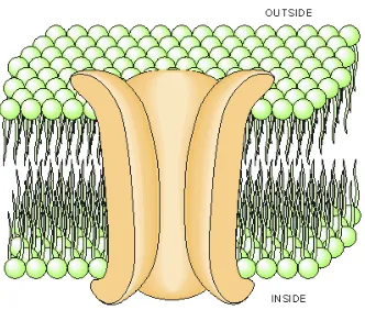
2.1.1 The Cell Membrane

(46)

phosphoric acid and fatty acids called glycerides (see Figure 2.3). The head of this molecule is phosphoglyceride, which is hydroφlic. The tail consists of hydrocarbon chains which are hydrophobic. This polar structure give rise to the elementary cell membrane structure.

If fatty acid molecules are placed in water, they form clumps (see Fig. 2.1.1(B)), with the hydroφlic acid heads attracted to water on the outside, and the hydrophobic hydrocarbon tails repelled by water on the inside. If these molecules are very carefully placed on a water surface, the hydroφlic heads will be attracted to the water molecules and the tails repelled outside of the water boundary (See Fig. 2.1.1(C)). If we pac The acid heads would protrude into the water on each side and the hydrocarbons would fill the space between. This bilayer is the basic structure of the cell membrane. Another stable form in water is a bi-layer structure shown in Fig. 2.1.1(D). At relatively low concentrations, fatty acids will form micelles, which can be thought of as tiny spheres of fatty acids. At higher concentrations and under the appropriate pH conditions, fatty acids micelles can form vesicles, which is the bilayer structure described above. Such bi-layer vescles are the basic structure of a cell membrane.

In the cell membrane there are pore-forming proteins making up what is called ion channels. From the bio-electric viewpoint, the ionic channels play an important role in

(47)

[image:47.612.128.521.146.392.2]

flow of these ions forms the basis of bio-electrical phenomena. Fig. 2.1.2 illustrates the construction of a cell membrane.

Fig. 2.1.1: A diagram illustrating how the phosphoglyceride (or phospholipid) molecules behave in water.

[image:47.612.242.408.460.601.2]

(48)

2.2 Sub-threshold Cell Membrane models

By regulating ion movements between the extracellular and intracellular spaces, the cell membrane plays an important role in establishing the resting and active electrical properties of an excitable cell. The ease with which an ion crosses the membrane, the membrane permeability differs significantly within an ion channel, this characteristic is

named as the ion channel's selective permeability. Activation of a cell affects its ion channels' behavior by altering these permeabilities. Another important consideration for trans-membrane ion movement is the fact that the ionic composition inside the cell differs greatly from that outside the cell. Consequently, concentration gradient is the driving force for all permeable ions that contribute to the net ion movement or flux.

Due to the selective permittivity, certain species of ions tend to accumulate at the inner and outer membrane surfaces (a diffusion process), which establishes potential difference, hence an electric field within the membrane. This electric field become the driving force for additional ion flow. Thus to describe membrane ion movements electric-field forces as well as diffusional forces should be considered. Equilibrium is achieved when the diffusional force balances the electric field force for all permeable ions.

(49)

2.2.1 Nernst Equation

If we consider one kind of ion, the Nernst equation gives the equilibrium voltage associated with a given concentration. The Nernst equation is derived from the electric field force and the diffusion force. For a more rigorous thermodynamic treatment see Katchalsky and Curran 1965 [32].

The current (ion flux) due to the electric field can be written as:

2.2.1.1

where

The current (ion flux) due to diffusion force can be written as:

2.2.1.2

where

(50)

2.2.1.3

where

At equilibrium the two current will balance out and the total current for the kth ion species is zero:

2.2.1.4

Separating out the potential gradient and integrate over the membrane thickness we obtain:

2.2.1.5

where i stands for intracellular space and o stands for extracellular space. Carrying out the integration in 2.2.1.5 we have:

2.2.1.6

where ci,k and co,k are the intracellular and extracellular concentrations of the kth ion

respectively. The voltage across the membrane is defined as PhiΦo – PhiΦi, rearranging

2.2.1.6 with this notion we have:

(51)

where

We now have arrived the Nernst equation. If we take the human body's normal temperature 37 °C (310 °K), and +1 for the ion charge, and write 2.2.1.7 in base ten logarithm form. We obtain a simply form for human cell membrane voltage:

2.2.1.8

So for all living cells at equilibrium, we can estimate their voltage between the cell membrane expressed as in 2.2.1.8. This voltage is called the resting voltage or resting potential.

Similarly if we consider all three major ions involved a resting voltage can be derived in the following form David Goldman (1943) [33] and Hodgkin and Katz (1949) [34]:

(52)

Substiting with human body's normal temperature and +1 for charge for Na+_{, K}+ _{and -1}

for Cl-_{, we have:}

2.2.1.10

The resting voltage of a neuron cell is about -70m, and about -95mV for a skeletal muscle cell. The resting voltage is important because a change in the resting voltage over a threshold will activate an excitable cell. Stimulation based applications inject high level currents so that the desirable cells (neuron cells, muscle cells etc.) are activated. For the applications of EIS and EIT we will be injecting <10mA alternating current which introduces very low potential gradient across the membranes, equilibrium state is assumed. As we will discuss in the following section, in the frequency we apply (1Hz – 250KHz) the cell's capacitive behavior is from the change of distribution of ions at the membrane on the inner-cellular and the intracellular side.

2.3 Tissue as a Volume Conductor

(53)

In most tissues we are interested in, it can be assumed that individual cells are roughly spheres with a diameter of around 10 µm. The cells are stacked together a lot like bricks and are held together by tight junctions (analogous to "spot welds"). In addition, there are gap junctions acting as channels for inter-cellular communication. The gap junction is a

direct inter-cellular providing paths for ions and small molecules to travel between neighboring cells. Since such paths are limited in numbers and have very small cross-sectional areas, the effective junction resistance is rather large. In fact, the net junction resistance between two adjoining cells is thought to be in the same order of magnitude as the end-to-end resistance of the myoplasm (extra-cellular electrolyte) of either cell. It is worth mentioning though without the junction gaps among cells the effective resistance is several orders of magnitude higher for ions to go through the bi-layer fatty acid membrane.

When studying a tissue comprising many cells, the complex tissue may be replaced by intracellular and interstitial continua. The electrical conductivity and permittivity of the continua represent suitable average of the actual structure. The membrane separates both domain at each point. This model is known as Bi-domain Miller and Geselowitz, 1978; Tung in 1978 [35].

(54)

Fig. 2.3.1: Diagram of equivalent circuit of a cell model (overlaid with the cell structure). Re is the extra-cellular resistance, Ri is the intra-cellular resistance, Rm is the membrane

resistance and Cm is the membrane capacitance (image from Webster 1990).

With many cells in the tissue, we consider the tissue to have a effective point wise conductivity and permittivity distribution.

Frequency dependent of Tissue's Dielectric Behavior

(55)

molecules. Fig. 2.3.1 shows a representative plot of the permittivity change vs. frequency. The frequencies we applied in this thesis are under the α and β dispersion range.

Fig. 2.3.2: Permittivity variation of a tissue as a function of frequency [37]

An electric model of such point-wise premittivity's frequency dependence can be written as below [38]:

2.3.1

where ε_∞ is the high frequency permittivity at which no polarizable element is able to

(56)

C h a p t e r 3

ELECTRICAL IMPEDANCE SPECTROSCOPY

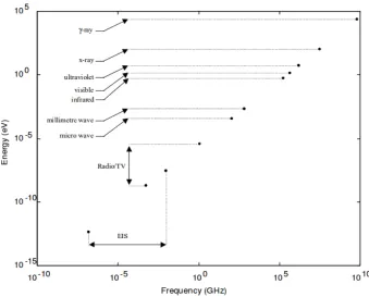
The world we live in is filled with Electromagnetic (EM) waves or EM radiation. The amount of energy such waves carry follow Planck's Equation E=hv, where v is the frequency of the wave and h=6.626x10-34_{is the Plank's constant (see Fig. 3.1). EM waves}

in different frequency bands display different characteristics based on the amount energy they carry. For instance, very high frequency EM waves are ionizing, as the frequency drops the waves become non-ionizing. An ionization wave is usually considered to have above 10eV in energy which includes the extremely high end of the spectrum to higher frequencies of ultra-violet light. The spectrum used in Electrical Impedance Spectroscopy (EIS) is considered within the radio frequency and very low frequency (VLF) bands and are non ionizing, namely 1Hz – 250KHz range. In EIS we study the interaction between alternating electric field and biological tissue in such frequency band.

(57)

[image:57.612.172.511.229.502.2]

obtained will be the same. This technique is actually being used in many commercialized EIS systems to insure the measurement data is within the linear region. The applied voltage or measured voltage due to current injection to stay in the linear region is usually considered to be <10mV.

Fig. 3.1: Energy vs. frequency band for Electromagnetic waves.

3.1 Concept of AC impedance

(58)

biological changes in the cell (surface and volume changes, phase transitions, electrolyte oxidation/reduction etc.) we can see the tissue as a passive linear volume conductor and Ohm's law applies. Then the voltage measured across tissue is also a sinusoidal function of the same frequency. If we express the current and voltage in tensor form we have:

3.1.1

3.1.2

Where ω is the radial frequency and θ is the phase delay. Then by definition, the impedance is the quotient of voltage and current:

3.1.3

or:

3.1.4

We call |Z| the magnitude of the impedance and θ the phase. If we have a purely resistive load then 3.1.4 reduces to Ohm's law in DC form R=V/I, and phase is zero. However real tissues possess capacitive characteristic as well as resistive so the impedance is complex.

(59)

The sensitivity distribution is crucial to understanding how the transfer impedance is related to the tissue admittivity. For any non-regular geometries we Let's consider a tissue volume with a certain admittivity distribution γ, when we inject an AC current I through a drive electrode pair, and measure voltage V. We have the transfer impedance Z defined as:

3.2.1

Now if the conductivity distribution γ is perturbed with δ γ, assuming linearity within the tissue volume, the impedance now becomes:

3.2.2

or

(60)

We can see that the change in transfer impedance is caused directly from change in voltage. We define the perturbation of voltage caused by the perturbation of admittivity to

be the sensitivity distribution: 3.2.4

In order to derive the sensitivity distribution, we consider the divergence theorem in an a closed volume region Ω, whose boundary ∂ Ω is a piecewise smooth surface (Fig. 3.2.1), if we imagine to inject uniform current I into the drive pair and sense pair respectively, then the following relation holds as shown in 3.2.5.

3.2.5

(61)

Fig 3.2.1: volume conductor with four electrode. A and B are the drive electrodes and C and D are the sense electrodes.

Taken the boundary condition into consideration, no current induced by the drive pair normal to the boundary occurs except at the driving electrodes A and B, hence the left-hand side of equation 3.2.5 becomes:

3.2.6

Similarly if we switch s and d in 3.2.5. and we obtain:

3.2.7

(62)

3.2.8

Now if we Iφd and Iφs are equal and then the voltages observed on the other pair would be equal. We have arrived the reciprocity principle [40], namely if the same voltage will be measured if we switch the drive and sense pairs.

We can divide both sides by I2_{in 3.2.6 and rewrite the potential gradient in terms of}

Ohm's law:

3.2.9

then we arrive at the formula for trans-impedance Z in an arbitrary volume conductor:

3.2.10

If we inject unit current then Z simply becomes:

(63)

Above representation of the trans-impedance implies that with four point electrode EIS the measured impedance is the integration of the point-wise resistivity (1/admittivity) scaled by the dot product of the current densities of the drive pair and sense pair. The reciprocity theorem is also obvious here because switching the drive and sense electrode pairs will not change the trans-impedance.

If we combine the drive and sense electrodes, we arrive at the trans-impedance formulation of the 2 electrode scheme:

3.2.12

With two electrode EIS, the current drive and sense current densities are identical and hence we have a strictly positive scaling factor shown in 3.2.12.

With small perturbation in the admittivity, we will have perturbation in measured voltage V.

(64)

3.2.13

Hence the sensitivity field can be expressed as:

3.2.14

Here we see, similar to the Trans-impedance, the sensitivity distribution is the integration of the dot product of the shape function of the gradient of the electric potential of the drive and sense pair. Depending on the position of the electrodes, unless two electrode measurement is carried out, the sensitivity distribution in certain areas can be zero or negative. This indeed creates complexity in attempting to correlate tissue properties to their trans-impedance. One of the most fundamental design principals is to design the positioning of the electrodes such that positive, and ideally uniform sensitivity distribution is achieved. Chapter 5 discusses this aspect in detail.

3.3 The electrode-electrolyte interface

(65)

is far from the ideal case. At initial contact, due to mismatch of the Fermi-levels in the electrode and the electrolyte, current flow will occur. Along with other reasons (adsorbed atoms on the electrode surface for example), a “double layer” establishes at the interface upon equilibrium. This double layer differ in electrical, compositional and structural characteristics.

(66)

Fig. 3.4.1: Esin and Markov, Grahame, and Devanathan model. [44]

The equivalent circuit is two capacitors in series:

3.4.1

where C is the total double layer capacitance of the double layer capacitor, C1 is the

capacitance of the inner Helmholtz layer which can be roughly modeled as a plate capacitor, and C2 is the outer Helmholtz layer whose capacitance changes mainly with the

concentration of the electrolyte solution. As the solution concentration increases the diffusion layer becomes small and hence C2 becomes large, so the 1/C2 term drop out in

(67)

concentrations the outer Helmholtz diffusion layer can be large hence C2 dominates the

double layer capacitance. The latter is the case for intracellular electrolyte.

Equivalent circuit model of the double layer

In addition to the double layer capacitance, there is also DC resistance due related to ion movement etc. Equation 3.4.2 shows the simplified equivalent circuit model at the electrode-electrolyte interface [45].

Fig. 3.4.2: Randle's circuit

Cdl is the double layer capacitor, the resistor in series Re is the electrolyte resistance due

to ion movement, Rt is the active charge transfer resistance associated with reduction/oxidation (redox) chemical reaction and W is an element of diffusion of such chemical reagents and is called Warburg element. In the case of small voltage and current perturbation we assume there is no redox reaction hence the parallel resistance is not existent. Fig. 3.4.3 shows the equivalent circuit in small perturbation case such as EIS.

(68)

In addition, through experiments the double layer capacitor is more appropriate replaced with a constant phase element. It is an empirical model with a constant phase that is < 90 degrees.

3.4.2

where ZCPE is the constant phase element, n is between 0 and 1, and the phase is 90*n. We can see that this non-ideal capacitor has resistant elements also with less than perfect phase. Such empirical correction is based on the observation of a depressed Nyquist plot, which will be talked about in the following section. Although the definitive explanation is still in debate it is in general agreement that the phase depression is due to some kind of dispersion at the electrode surface.

Ag/AgCl electrode

So far we have focused on polarizing electrodes such as most metals, another electrode that is largely used for non-invasive Bio-electricity applications is made of Ag/AgCl (for example electrodes used for ECG recording). Ag/AgCl are also used as the reference electrode for 3 electrode setup and as the reference electrode in pH meters. In contrary to the metal electrodes, these electrodes function as a redox electrode with no double layer charge accumulation. The reaction is between the silver metal and silver chloride salt.

3.4.3

(69)

With an overall reaction of:

3.4.5

The fact that Ag/AgCl electrode is a redox electrode makes it important to look at the reaction kinetics and obtain its frequency response over the EIS band. In the figure below shows a magnitude Bode plot of an Ag/AgCl in 0.01M HCL.

Fig. 3.5.3: Effect of Structural Design of Silver/Silver Chloride Electrodes on Stability and Response Time and the Implications for Improved Accuracy in pH Measurement [46]

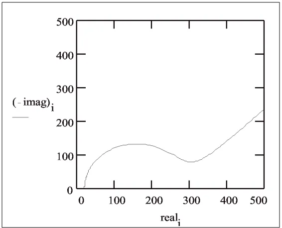
3.4 Bode plot and Nyquist plot

(70)

capable of displaying a wide range of system response vs. a wide range of frequencies. Bode plot isused to assess stability of poles and zeros of a system. In EIS the impedance magnitude is usually shown as a log-log bode plot while the phase is shown on a semi-log scale plot.

Nyquist plots are parametric plots of a system response. It is often used in a feedback system to assess stability. Here in EIS, The x axis of a Nyquist plot is the real component of the impedance and the y axis the imaginary. Each point on the plot is a complex impedance measured at a certain frequency.

(71)

Fig. 3.5.1.: Simulated amplitude Bode plot (up) and phase Bode plot (down) based on Randle's circuit in Fig. 3.4.2

(72)

[image:72.612.178.461.139.368.2]

The capacitance per unit area is dependent on the kind of metal and the electrolyte. A rule of thumb for gold electrode is 60 μF/cm2_.

Fig. 3.5.2: Simulated Nyquist plot of a of an ideal Randle's circuit based on Randle's circuit in Fig. 3.4.2.

In the Nyquist plot we can see a semi-circle connected to a line of 45 degree angle (equal dynamic phase delay). The 45 degree line occurs in the low frequency region and is associated with the Warburg element. As the frequency increases the double layer capacitor's impedance becomes dominant and we show a typical semicircle of RC circuit. At extremely high frequencies we arrive at the left end of the semicircle, at this time only the series resistance Re is effect. Without the active reaction parallel circuit the Nyquist

(73)

clockwise [47], hence instead of having a 90 degree angle. The CPE's phase delay is less than 90 degrees.

3.5 Lumped circuit model

If we aproximate the tissue to be isotropic and uniform and has a regular shape of Fig. 3.5.1, with metal plate electrodes on each end (see Fig. 3.5.1).

Fig. 3.5.1: tissue and electrode model for EIS measurement

The equivalent of such model with lumped circuit elements can be shown in Fig. 3.5.2.

Using a simplistic model, the cross section A is comprised two materials: the cells taking up A1, and the extracellular electrolyte taking up A2, where A1 + A2 = A. The cell can be

modeled as a capacitor (double layer at the cell membrane) and resistor (inner-cellular electrolyte), lump up the cells we get R1 and C to model the cells (see Fig. 3.5.2). The extracellular electrolyte can be modeled with resistor R2 (Fig. 3.5.2). Now we can derive the equivalent circuit model for tissue to be the following.

(74)

Fig. 3.5.2: equivalent circuit of tissue and electrode model

3.5.1

Where 3.5.2

3.5.3

3.5.4

With the constant phase element model for the electrode-electrolyte interface in 3.3.2 in series, we have the Bode plot of the equivalent circuit. We can see three corners which are determined by the double layer impedance and the tissue impedance. The calculation of the corner frequencies are shown in Fig. 3.5.3. The second corner and third corner are closely related to both the tissue's inner and intra cellular properties (for example the

(75)

content of the cell, the cell geometry, and the packing density etc.), hence the tissue's impedance properties can be correlated to corner frequencies along with the levels of the flat band between first and second corner. In Chapter 4 we will see the biological tissues follow roughly the shape. The exact corner frequencies are determined by the electrode effective surface area and the tissue itself.

(76)

C h a p t e r 4

ELECTRICAL IMPEDANCE TOMOGRAPHY

In electrical impedance tomography (EIT) voltage data measured at the boundary of a conductive domain are used to reconstruct the spatial distribution of its electrical conductivity (admittivity). The technique has been widely applied in geophysics such as oil exploration, and nondestructive testing of materials [48-52]. EIT has been recently applied in the bio-imaging field such as bed-side lung ventilation monitoring [53,54]. In this chapter we explore the possibility to apply EIT in novel applications of vulnerable plaque imaging and fatty liver early detection, both of which are closely related diseases and can become fatal if not detected in time and yet treatable if detected early.

4.1 The instrumental setup

(77)

[image:77.612.109.537.302.535.2]

currents of 1khz – 100khz range. The upper limit was determined by the current source Keithley 6221 to be 100khz, the maximum sampling rate of the NI DAQ is 1M samples/sec so it can achieve theoretically 500K samples/sec, or practically 200K samples/sec (Nyquest rate of ½ sample frequency is hard to achieve in practice, it is good to leave some margin). Although it is recognized that recent years have seen developments and commercialization of several new multi-frequency EIT systems that are capable of scanning a wide range of frequencies [55-57].

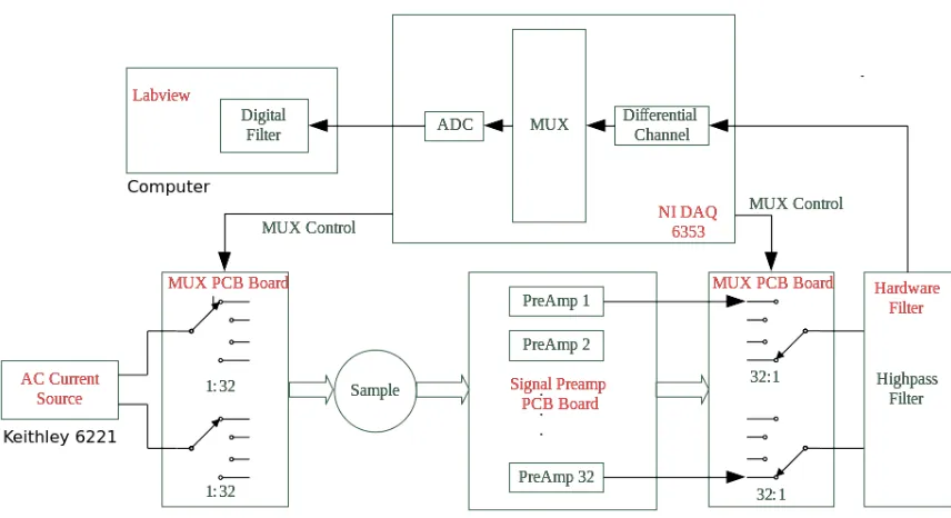
Fig 4.1.1: System diagram of the Labview Based system.

(78)

actually current injection is by AC current source Keithley 6221 (Keithley, USA). For the voltage measurement, each channel goes through a pre-amplifier stage prior going through the multiplexer board, the selected signal then goes into the hardware filter. The filtered signal then feeds into the DAQ differential analog channel to be read by the Labview program. An additional bandpass digital filtering is performed for the voltage reading in Labview.

Fig 4.1.2: Pre-amp circuit diagram. RG=200Ω (0.1%, 15 ppm/oC) Gain = 1+9.9k

Ω/RG=50.5x

(79)

[image:79.612.108.540.113.362.2]

Fig 4.1.3: Time domain waveforms. Upper left: Signal out of pre-amp (blue), signal out

of hardware filter (red). Lower left: DAQ settings, sampling rate is 100Khz. Voltage range is +/-0.1V. Upper right: signal after pre-amp, before hardware filter. Lower right: signal out of hardware filter. Noise performance of Swisstom and Labview System.

Noise performance is critically important for the reconstruction quality. Higher noise means we need to use bigger regularization parameter which compromises the fitting of the data that resembles the conductivity distribution.

We define the noise in each voltage channel (totaling 32x32 = 1024 channels) to be the quotient of the the average of the signal over 10 frames of data to the standard deviation of such data.

(80)

Where i= 1,2,…,1024. And SNR in db form is 20 log10(SNR).

[image:80.612.153.472.288.523.2]

The following Figures show the noise comparison of Swisstom system in noise performance.

(81)

4.2 The mathematical framework

EIT has seen numerous theoretical and computational developments since the beginning of its time in the 1980s [58-62] However, two fundamental challenges remain that limit EIT's accuracy and resolution, namely the nonlinearity of the forward problem and ill-posedness of the inverse problem. From the mathematical prospective, this inverse boundary value problem, formalized by the Caldéron's first paper on EIT of [58], presents a number of implications on the existence, uniqueness, and numerical stability of the solution [62]. Although the issues of existence and uniqueness can be eradicated with reasonable assumptions about the conducting body, instability causes the solution to be extremely sensitive to noise in the voltage data. Such instability is caused by the severely lack of full boundary voltage data. To alleviate the ill-posedness one usually resorts to implementing some type of regularization strategy to stabilize the solution based an a priori knowledge about the conducting body (differentiability, smoothness etc.)

The inverse problem is usually solved as an optimization problem with constrained (regularized) Gauss-Newton (GN) type solver. In order to calculate the residual error in the above inverse problem, a forward problem also needs to be solved. In the sub sections below we layout the mathematical framework of the EIT problem.

4.2.1 The inverse problem

(82)

“forward problem” obeying the governing Maxwell equations (more details in 4.2.2). 4.2.1.1

To take a Gauss-Newton approach, the solution of σ would be which that minimizes the

L-2 norm of the error: 4.2.1.2

Hence the objective function to be minimized is:

4.2.1.3

If we take the first order of Taylor series expansion of the forward problem function can be approximated as:

4.2.1.4

Then the objective function becomes:

4.2.1.5

To minimize PhiΦ, we set and solve for σ, from 4.2.1.5 we

have:

(83)

Solution in 3.2.1.6 shows the scheme of the so called “absolute imaging”, where only one voltage data set is measured and subtract by the calculated voltage data set.

Since the nature of the forward function is not linear, solving 3.2.1.6 iteratively are needed in order to converge σ to a meaningful solution. However, since error from the forward calculation (mainly due to geometry mismatch especially around the electrodes) is added to the measurement noise thus influences the direction of the solution in each step, convergence to is not guaranteed [63-65]. However the GN algorithm converges well if the forward problem is very close to linear, which is true when only when the σ perturbation is small. Then the forward problem can be written as :

4.2.1.7

And the solution becomes:

4.2.1.8

This has inspired the so called “difference imaging”, which measures two data sets before and after a small σ change. Hence the forward problem can be approximated as linear and the difference in σ is computed:

(84)

In the difference imaging scheme, the calculated voltage set is not present and does not influence the solution direction. In fact with small σ perturbations the one-step solution is usually satisfactory.

Regularization

Above we have arrived at the unconstrained GN solver. However in practical situations the unconstrained GN form cannot be used due to the following 2 reasons: First, since J is far from full rank JT_{J is not full rank, hence inverse of J}T_{J does not exist. Second, due to}

the ill-posed nature of the inverse problem, the solution σ is heavily sensitive to the perturbation in measurement voltage V, which means a small noise in V can result in a big change in the solution σ. The treatment for such condition is to introduce a constraint so that the solution will favor those that we prefer.

4.2.1.10

Here we add a constraint term to the objective function. The term in 3.2.1.10 is the L-2 norm of the solution σ. This means we will punish the large conductivity spikes in the solution space. The coefficient lambda is the regularization parameter, we will be setting this parameter such that we balance the trade off between fitting the error and constraining the solution from undesired properties.

(85)

4.2.1.11

The above form is known as the Tikhonov Regularization. The term Γ is introduced to enable us to select more properties of the σ. For example if we know the solution is smooth Γ can be a Laplacian operator to punish the non smoothness in solutions. Or if we know in a priori that certain area of the conductivity is the same or similar Γ can be a “weighted” Laplacian operator that punishes non-smoothness heavily in these regions. This is applicable in medical imaging where EIT is to obtain the conductivity information of certain organs, and information of location of the organs may be obtained a priori with other imaging modality (CT, ultrasound, etc.). In this scenario the conductivity of the organs of interest may be determined more accurately with such a priori information (details in following experimental section).

The solution to 3.2.1.11 after setting the gradiant to zero is the following:

4.2.1.12

Similarly the difference imaging solution under the linearized forward problem becomes:

(86)

4.2.2 The forward problem

The forward problem is that given conductivity distribution of a domain, under certain current excitation pattern we find the voltage distribution on the boundary of the domain. To write out the forward problem function explicitly 3.2.1.1 can be expressed as:

4.2.2.1

Where I is the current injection pattern. According to linearity of Maxwells equations we can write this function as matrix form :

4.2.2.2

Where Upsilon is the the linear operator that is determined by σ. It is the Dirichlet to Neumann operator associated to conductivity σ. You may encounter Upsilon in other names such as the system matrix, the stiff matrix, etc. As we have seen in section 3.2.1 each GN inverse step involves solving for this forward problem and/or the Jacobian derived from this forward problem. In the following section will show the formulation of such Upsilon operator and the method to solve it numerically.

(87)

In order to formulate Γ we first introduce the governing equations for this problem. We assume the biological domain is source free. Then within the domain the Laplace equation holds:

4.2.2.3

Of course in a human body we will have heart ECG and muscle EMG inevitably occurring. These electrical signals are modeled as electrical dipoles propagating at the signal front. The electrical dipole is formed due to the reverse polarity of the cell membrane in the activated cell. It is apparent that the dipole distance is on a cellular level (distance between two cells) and is far less than the distance we observe from. Hence we can use the dipole's far field formulation as the potential field solution. One can verify that a dipole's far field solution approaches the Laplace equation 4.2.2.3.

In addition to satisfying the Laplace equation, at the boundary we should satisfy:

4.2.2.4

4.2.2.5

(88)

Where Γ_el is the boundary where electrodes are present. The boundary conditions simply means that the current flux at the boundary is zero where there is no electrode and total current under a certain electrode should sum up to be Il, the current on the lth

electrode based on the current injection pattern I, where l = 1, 2, …, L. The third boundary condition in 3.2.2.6 is to specify that the potential on the lth electrode Vl, is the

potential u on the boundary plus the potential difference due to existence of contact impedance. Above 3 boundary conditions form the so called “complete electrode model”. One point that is worth noticing is that, however, in the complete electrode model we assume the conductivity σ, or 1/σ as zl , is the same within all points of the boundary

under an electrode. This may not be the case under practical situations in tank experiments as an electrode surface may not be in the same condition everywhere. This can lead to additional errors in forward calculation as 3.2.2.6 is not accurate anymore. However it is assume Ag/AgCl ECG type electrodes have uniform conductivity and the skin underneath is in similar condition and thus has uniform conductivity.

It has been proven that with vanishing currents on the boundary surface and a defined ground 4.2.2.3 – 4.2.2.6 has unique solution [66]. Hence we have simply:

4.2.2.7

(89)

To satisfy 4.2.2.7 we will balanced charges injected and for we define the ground to be the sum of boundary potentials in 4.2.2.8.

Numerical method

In order to solve for Γ numerically with FEM techniques we express the governing function in its weak form, by taking the inner product of the Laplace equation with a test function φ:

4.2.2.9

Although the detailed reason is out of scope of this thesis, the rationale to solve the weak form instead of the strong form of the PDE is that by introducing the weak form we are able to relax the smoothness requirement of the solution . This is done with integration by parts. With integration by parts from equation 4.2.2.9 and assume u = 0 at ∂ Ω we arrive at the following equivalent form:

4.2.2.10

We can see that after integration by parts the solution u is no longer required to be twice differentiable, but rather once differentiable, hence the solution space is relaxed.

(90)

4.2.2.11

Then the solution u can be expressed as a linear combination of the basis function weight coefficient Ui, where i = 1, 2, …, n:

4.2.2.12

Now we write the weak form 4.2.2.10 in the terms of the basis function 4.2.2.12, and apply green's theorem, the left-hand side becomes:

4.2.2.13

Where j is one particular node, and 4.2.2.13 applies to all nodes individually in the domain and at the boundary. Apply boundary conditions 4.2.2.4 – 4.2.2.6 to all j we arrive at the matrix form of 4.2.2.13.

4.2.2.14

4.2.2.15

(91)

4.2.2.17

4.2.2.18

U contains the coefficients to all the nodal potential basis, and V is a subset of U and contain coefficients of the electrode facing nodes. The top su