Conservative bounds for the pfd of a 1-out-of-2 software-based system based on an assessor’s subjective probability of “not worse than independence”

City, University of London Institutional Repository

Citation:

Littlewood, B. and Povyakalo, A. A. (2013). Conservative bounds for the pfd of a 1-out-of-2 software-based system based on an assessor’s subjective probability of “not worse than independence”. IEEE Transactions on Software Engineering, 39(12), pp. 1641-1653. doi: 10.1109/TSE.2013.31

This is the accepted version of the paper.

This version of the publication may differ from the final published

version.

Permanent repository link:

http://openaccess.city.ac.uk/2514/

Link to published version:

http://dx.doi.org/10.1109/TSE.2013.31

Copyright and reuse: City Research Online aims to make research

outputs of City, University of London available to a wider audience.

Copyright and Moral Rights remain with the author(s) and/or copyright

holders. URLs from City Research Online may be freely distributed and

linked to.

“not worse than independence”

Bev Littlewood, Andrey Povyakalo

Centre for Software Reliability, City University, London EC1V 0HB

Abstract

We consider the problem of assessing the reliability of a 1-out-of-2 software-based system, in which failures of the two channels cannot be assumed to be independent with certainty. An informal approach to this problem assesses the channel pfds (probabilities of failure on demand) conservatively and then multiplies these together in the hope that the conservatism will be sufficient to overcome any possible dependence between the channel failures. Our intention here is to place this kind of reasoning on a formal footing. We introduce a notion of “not worse than independence” and assume that an assessor has a prior belief about this, expressed as a probability. We obtain a conservative prior system pfd, and show how a conservative posterior system pfd can be obtained following the observation of a number of demands without system failure. We present some illustrative numerical examples, discuss some of the difficulties involved in this way of reasoning, and suggest some avenues of future research.

KEY WORDS: System reliability; Software fault tolerance; 1-out-of-2 system; Dependent failures; Subjective probability.

1

Background

The experimental results were confirmed in some contemporary theoretical modeling, which also provided a conceptual framework for understanding reasons for failure dependence (Eckhardt and Lee 1985; Littlewood and Miller 1989). The basic idea introduced by Eckhardt and Lee is that “problem difficulty” varies over the demand space: some demands are “intrinsically harder” than others. That is, it is harder to build a program that executes such a demand correctly (i.e. the chance of a particular program doing so is smaller). If channel A fails on a randomly selected demand, one should conclude that this was probably a difficult demand and thus the chance of channel B failing on the same demand is greater than it otherwise would be: i.e. this conditional probability of B failing is great than B’s marginal pfd. The result is that there is positive association between channel failures, and the 1-out-of-2 system pfd is greater than it would be if independence of failures could be assumed.

Littlewood and Miller generalize this result to the case where diversity is forced by employing deliberately different “methodologies” to develop A and B. In this case the variation of difficulty for A will generally be different from that of B: demands that are hard for B may be easier for A and vice versa. It is shown that in this case the association between channel failures can be either positive or negative – i.e. it is possible to do better than the case of independence (the 1-out-of-2 system pfd can be smaller than the product of the two channel pfds). Whether it is practically feasible to force the methodologies to be sufficiently different that the channels exhibit such negatively associated failure behaviour remains a moot point. If it is possible, it is unlikely that one could be certain that negative association of failures had been achieved for a particular pair of channels.

In summary, then, the position is this. Whilst there is evidence that this approach may be effective – in some average sense – in achieving system reliability, it is difficult to assess the reliability of a particular design-diverse system. This is because the level of association between the failures of the diverse channels will not be known – in particular it cannot be assumed that they will fail independently. These problems of assessment are important because they are a barrier to the use of what is otherwise one of the most promising approaches to very high system reliability.1

An interesting way around this difficulty arose in some discussions the authors had with engineers involved in the licensing of a 2-channel, 1-out-of-2 protection system. The pfd of the system was required to be no worse than 10-6

. It was expected that there would be extensive analysis of the “diversity-seeking” decisions involved in the designs of the two channels, so it may be reasonable to conclude that any dependence between the channel failure processes would be modest. The pfd claims for the two channels – 10-4

and 10-2

– were believed to be very conservative, sufficiently so that taking the product of these, it was claimed, would give a conservative value for the system pfd even in the possible presence of some positive dependence between the channels.

The difficulty with this kind of reasoning, we think, is that it makes a trade-off between very different things: pessimism in channel claims against optimism in

1 _{Although it should be said that other approaches to achieving high reliability also pose great difficulties in}

claims about joint failure behaviour. It seems reasonable to ask how optimistic the independence claim is (i.e. how dependent the channel failures actually are) and how pessimistic the channel claims are – and then to ask whether the latter is sufficient to overcome the former. A more subtle critique of this kind of reasoning would ask for confidence in claims to be made explicit (and preferably quantitative): e.g. what confidence could be placed in the system pfd claim of 10-6

given particular evidence of trade-off between pessimism about channel claims and optimism about channel dependence? This issue of “confidence” is often neglected in claims about even life-critical systems: for example, standards such as IEC16508:2010 treat the reliability levels (such as pfds) associated with Safety Integrity Levels (SILs) as if these could be claimed with certainty. See (Bloomfield and Littlewood 2003) for a discussion of the wider issues here.

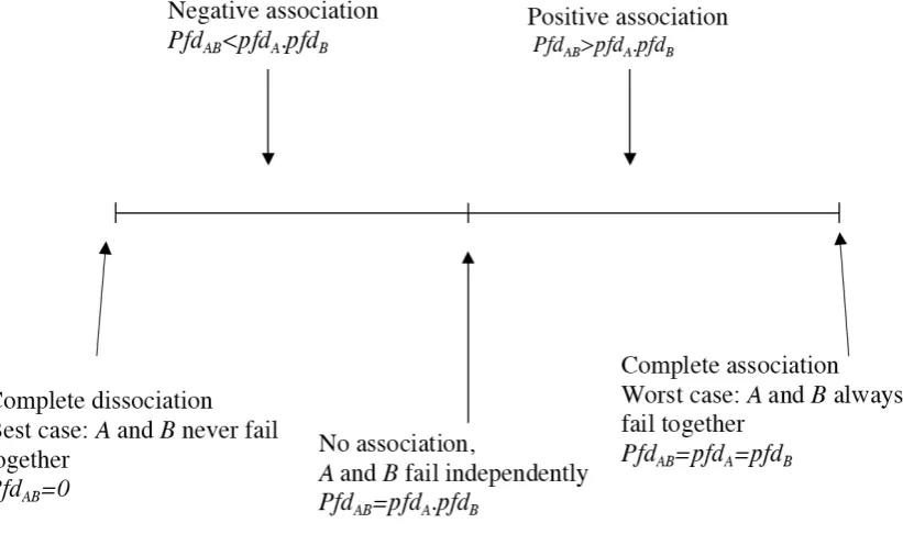
[image:4.595.104.515.466.709.2]

In the work reported here we aim to put this kind of “trade-off” reasoning on a more rigorous footing in order to make conservative claims for multi-channel systems in the presence of likely channel failure dependency. We begin with a brief examination of the nature of “association”, or dependency, between channel failures, with the intent of explicitly modeling the uncertainty here.

Figure 1 illustrates the spectrum of possible dependence between channel failures. It ranges from a best case where there are no coincident failures (the failure regions of the input space for channel A and channel B are disjoint), to a worst case where all failures are coincident (the failure regions are identical). It is clear from the figure that independence is a very special case: it is just one point in the “middle” of this spectrum.

For a particular pair of channels, there will be a point on the spectrum, x, that represents the degree of association between failures of that pair. We might express this numerically, for example, as the ratio pfdAB/pfdA.pfdB.

The important point is that there is uncertainty about the value of x: an assessor could not be certain that x took a particular point value on the spectrum. It is appropriate, therefore, to treat x as a random variable, and an assessor can be expected to have some prior beliefs about it (such beliefs might be based, for example, on knowledge of how the two channels were developed). As is often the case, it seems unlikely that an assessor would be able to state a complete prior distribution for x. We propose to examine the case where the assessor can tell us a single point on this distribution, specifically his probability that x is not greater than 1. This is his confidence that the association of channel failures is not positive in Figure 1 (that pfdAB is not greater than pfdA.pfdB), i.e. channel failures are not worse than independent (NWTI).

Notice that in this case the assessor is expressing his belief about x as a probability associated with an interval on the spectrum of dependence. This seems more reasonable than associating a probability with a point on the spectrum – in particular with the “independence” point, x=1. We might be prepared to regard as reasonable an assessor’s claim of the kind “I am 90% sure that x is no greater than 1”, but not a claim such as “I am 90% sure that x=1”. More formally, we assume that the distribution representing his belief about x is absolutely continuous, and thus has zero probability mass at a point.

We believe that the most convincing use for the results in the rest of the paper lies in allowing assessors (or, more importantly, assessors of assessors, such as regulators) to challenge claims based on the informal trade-off arguments described above: “If your channel claims are pessimistic by this amount, and you have seen this amount of failure-free testing, then it follows that your doubt in NWTI needs to be smaller than this”.

2

Model based on an assessor’s level of confidence that “channel

failures are not worse than independent”

The basic idea here is similar to that we proposed in (Bishop, Bloomfield et al. 2011). In that paper it was shown how to obtain a conservative pfd for a single channel based on an assessor’s limited prior belief, together with some failure-free operational testing. It is well-known that people find it hard to express their subjective prior belief as a complete distribution for an unknown parameter (in this case channel pfd). Instead, in this work it was assumed that the assessor was only able to state a single percentile (i.e. single point on the abscissa of his subjective cumulative distribution) for his prior belief about the channel pfd: thus he might just be able to say, for example, “I am 90% confident that the pfd is smaller than 10-3

”, more generally provide a single pair of numbers (x, y) representing his subjective probability (1-x) that the pfd is smaller than y.

of the example of the previous paragraph, this distribution is the one that places 90% of the probability at 10-3

and the remaining 10% at 1.

[image:6.595.186.407.218.543.2]

More surprisingly, it was also shown that following seeing the execution of some demands without failure, another 2-point prior distribution (one satisfying the assessor’s percentile constraint) gives the most conservative posterior mean pfd. The interpretation of this is that the assessor can treat this value as a conservative bound for his true probability of failure on demand – for example in a wider safety case.

Figure 2: from (Bishop, Bloomfield et al. 2011). At top is an ideal complete distribution for an assessor’s belief. However, he is unable to express the infinite number of probabilities implicit in this figure, and can only give us a single percentile (x, y) of the distribution: i.e. the area, x, to the right of a single point, y. Below is the most pessimistic of all possible distributions, f(p), that satisfy his expressed belief: it is obtained by placing all the probability masses associated with the intervals (0, y) and (y, 1) at the extreme right of the intervals (note that the bars here represent probability mass, in contrast to the probability density function in the upper figure).

1-dAB(0). That is, the probability dAB(0) is the assessor’s doubt, expressed as a probability, that the channel failures are independent or better2_.

That is, the assessor’s prior distribution, f(p), for the system probability of failure, PFDAB3_{, has a 1−d}

AB(0)

(

)

×100percentile at pfdA.pfdB, i.e.:

f(p)dp=

0 pfd_A.pfd_B

∫

P(PFD_AB≤pfd_A.pfd_B)=1−d_AB(0) (1)

We also assume initially, without loss of generality, that pfdA ≤ pfdB. Since we know that the probability of failure of a 1-out-of-2 system cannot be worse than the best channel pfd, we also have:

f(p)dp= 0

pfd_A

∫

P(PFDAB≤ pfdA)=1 (2)

which gives a second percentile of f(p). We thus have two percentiles of the assessor’s prior distribution for the system’s probability of failure on demand, PFDAB. In general, there will be an infinite number of potential prior probability density functions, f(p), that satisfy (1) and (2). It is easy to see that the most pessimistic of these is the 2-point distribution that has probability mass at pfdA.pfdB (with probability 1–dAB(0)), and probability mass at pfdA (with probability dAB(0)). The reasoning here exactly parallels that in (Bishop, Bloomfield et al. 2011), described earlier: the most pessimistic 2-point distribution is one that moves the probability mass in the intervals (0, pfdA.pfdB) and (pfdA.pfdB, pfdA) as far to the right as possible (i.e. to the right hand end of each interval).

Since the assessor’s probability that the system fails on a randomly selected demand is just the mean of his (in this case, prior) distribution of PFDAB, we have:

P(system fails on randomly selected demand)

=E(PFDAB| 0 failure-free tests observed)=pfdAB(0), say

= p.f(p)dp

0 1

∫

€

≤pfdA.pfdB(1−dAB(0))+pfdA.dAB(0) (3)

This bound is the value that the assessor can treat as his true (prior) probability of failure of the system on a randomly selected demand, and be assured that it is a conservative (although attainable) number.

Of course, this prior bound may not be of practical value – it may be very conservative for reasonable values of dAB(0). However, as in the case of a single system (Bishop, Bloomfield et al. 2011), things become more interesting and useful when evidence is available of extensive failure-free working of the 1-out-of-2 system.

2 _{The notation here anticipates the more general one we require later in the paper, when we show how such}

confidence/doubt changes as a result of seeing N failure-free demands. Here N=0.

3 _{We shall use, as far as possible, upper case letters to indicate random variables, and lower case letters to}

When N demands have been executed by the system, and no failures have been seen4_, the assessor’s belief about PFDAB changes from his prior distribution, f(p), via Bayes’ theorem. His posterior distribution is

f(p|N failure-free demands)= (1−p) N

f(p)

(1−p)N f(p)dp 0

1

∫

(4)

The assessor’s posterior probability of failure on a randomly selected demand is the mean of this distribution:

€

P(System fails on randomly selected demand |N failure - free demands) =E(PFDAB|N failure - free demands)

=

p(1−p)N

f(p)dp 0

1

∫

(1−p)N

f(p)dp 0

1

∫

(5)

The question now is which, of the infinite number of prior density functions f that satisfy (1) and (2), are the most pessimistic, i.e. maximize (5). In general there will be an infinite number of these. We can show that, once again, one of these is a 2-point distribution; i.e. this distribution has the same posterior expectation as the (many) other most pessimistic priors. This distribution has probability mass concentrated at pfdA.pfdB, as before, and probability mass concentrated at a point zAB(N), where zAB(N) is the value of z that maximizes the posterior mean:

€

FAB(z)=E(PFDAB|N failure - free demands)

= pfdApfdB(1−pfdApfdB) N

(1−d_AB(0))+z(1−z)N

d_AB(0) (1−pfdApfdB)

N

(1−dAB(0))+(1−z) N

dAB(0)

(6)

The conservative “true” system pfd is then the value (6) takes at its maximum, i.e.

€

E(PFDAB|N failure - free demands)≤FAB(zAB(N)) (7)

€

=pfdAB(N), say (8)

The assessor’s doubt that the failures of the two channels are NWTI changes as he observes N failure-free demands, from his prior belief dAB(0) to posterior:

€

d_AB(N)= (1−zAB(N))

N

d_AB(0) (1−pfd_Apfd_B)N₍₁

−d_AB(0))+(1−z_AB(N))N_d AB(0)

(9)

in an obvious notation. The conservative posterior distribution of the system pfd, (4), is a 2-point distribution with probability mass (1-dAB(N)) at the “independence” point, pfdA.pfdB, and probability mass dAB(N) at zAB(N), which has the mean given by (7). For proof of these statements, see Appendix.

The reader should note that “conservative” here refers only to the mean value of the system pfd: from the infinite number of prior distributions that satisfy the assessor’s

4 _{Note we are assuming at this point that only system successes/failures are observed, and not the individual}

expressed beliefs, (1) and (2), there is none that gives a larger posterior mean pfd than (8). The “conservative” posterior distribution here may not be conservative in other respects. For example, it has no probability mass to the right of the point zAB(N), which many assessors might regard as too optimistic.

3

Practical implications of the model: Examples

Consider the following simple illustrative example. Assume that pfdA = pfdB = 10-3 , the initial doubt, dAB(0) = 0.1, and that we see 2000 failure-free demands, i.e. N = 2000. We have:

pfdAB(0) ~1 10-4

, from (3) pfdAB(2000) = 2.063 10-5 dAB(2000) = 0.0365 zAB(2000) = 0.00054

What has happened here – are these results useful? Clearly, the assessor’s conservative “true” prior system probability of failure on demand, at approximately 10-4

, is not a very useful improvement on the single channel pfds. However, the conservative “true” posterior system probability of failure on demand, pfdAB(2000), is almost two orders of magnitude better than the crude bound 10-3

(the probability of failure of the best channel). It is also considerably better than the “black-box” 99% confidence bound 2.65 10-3

, which is obtained by treating the system as a single black box about which nothing is known except that it has survived 2000 demands without failure (Littlewood and Wright 1997).

Furthermore, confidence in “no worse than independence” of A, B channel failures has increased to over 0.96 from the assessor’s original 0.90. The right hand point, z, of the conservative 2-point distribution has moved to the left, closer to the “independence” point pfdA.pfdB.

In general, the final (conservative) claim for system pfd depends upon: the channel probabilities of failure on demand, pfdA, pfdB; the prior doubt, dAB(0), about the channel failures being no worse than independent; the number of failure-free system demands, N, that have been seen. One way the results of Section 2 could be used would be to see whether any points in this (pfdA, pfdB, dAB(0), N) space seem feasible. For example, given the values of pfdA, pfdB, dAB(0), we could see how many test cases need to be executed (and show no failures) to obtain a particular value of pfdAB(N): in many cases, such as reactor protection systems, the cost of generating test cases may be high so that a large N may be infeasible. Alternatively, given the values of pfdA, pfdB, N (where here N is regarded as the size of the largest practically feasible test set), we could calculate the required dAB(0) and ask whether such a belief could be trusted (for example, supported by evidence about the diversity-seeking decisions (Littlewood and Strigini 2000; Wood, Belles et al. 2010) taken during system design and build). We believe that using our approach to challenge parts of safety cases in this way may be its most useful contribution.

We shall illustrate the general approach via the real example of a safety-critical protection system discussed briefly in Section 1. The aim was to claim a pfd of 10-6 for the two-channel system, each channel of which is software-based. The individual channel pfds are estimated conservatively at 10-4

and 10-2

claim, 10-6

, is then obtained by multiplying these two channel claims. In our private discussions with safety engineers and assessors, we understood that the reasoning here is that “modest” dependence between channel failures will be more than countered by the conservatism of the individual channel pfd claims: the claim of 10-6 for the system pfd will then be conservative.

We have already expressed our scepticism about such a trade-off. We now sketch out how the system claim of 10-6

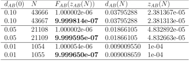
might be supported by the kind of reasoning of Section 2. In particular, we show how many failure-free demands of the system need to be observed to support the claim for different levels of doubt about “no worse than independence”, and different degrees of conservatism in the channel pfd claims. Table 1 shows the results of our analysis when the assessor believes the channel pfds are no worse than 10-4

and 10-3

respectively. For the three different values of an assessor’s doubt about NWTI, 0.10, 0.05, 0.01 respectively, the table shows the value of N for which the system pfd claim 10-6

can be supported. Thus, the number in bold for FAB(zAB(N)) in the second row of the table corresponds to N=43667, the smallest number of failure-free demands that allow a system pfd claim of better than 10-6

when the initial doubt is 0.10. These results are somewhat unforgiving: for the two most modest values of the doubt, the numbers of failure-free demands needed are rather high. This amount of operational testing may not be feasible for some applications. For example, it is an order of magnitude greater than what was feasible twenty years ago in the case of the Sizewell B PPS software (May, Hughes et al. 1995). However, there have been significant advances in computing speeds in the past twenty years, and much larger simulations are now possible: for example, 50,000 test cases may be generated as part of the assessment of the C&I functions of the UK’s proposed EPR (HSE 2011).

[image:10.595.134.437.522.619.2]

For the smallest doubt, 0.01 represented by the last two lines of the table, on the other hand, only 1055 failure-free demands are required, and this does seem sufficiently modest to be feasible in many cases.

Table 1 Required values of N (number of failure-free demands) to support a system pfd claim of 10-6 _{for different values of initial assessor doubt d}

AB(0). Here pfdA=10-4, pfdB=10-3.

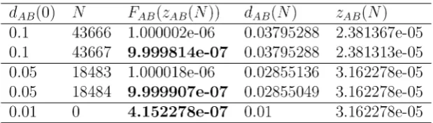
Table 2 shows the results for a similar calculation when the channel pfds are no worse than 10-4.5

and 10-2.5

respectively. As in Table 1, these numbers are chosen so that their product – the “independence” case – is 10-7

system pfd is better than 10-6

[image:11.595.134.444.144.232.2]

: this claim can be made simply from the prior beliefs about the channel pfds when the doubt about NWTI is 0.01.

Table 2 As Table 1, except pfdA=10-4.5, pfdB=10-2.5.

Finally, in Table 3 the results are shown for a calculation in which the channel pfds are no worse than 10-5

and 10-2

. Again the product – the “independence” case – has been chosen to be 10-7

.

Table 3 As Table 1, except pfdA=10-5, pfdB=10-2.

In this case the required conservative system pfd claim of no worse than 10-6

can be made for values of dAB(0) of 0.01 and 0.05 a priori, i.e. without seeing any failure-free working. Even when the doubt is 0.1, the required number of failure-free system demands is only 10642, which is more modest than the numbers required for the examples of Tables 1 and 2.

The results of Table 3 are less unforgiving than those of the other two tables. This seems to be because the channels are more asymmetric: channel A is much more reliable than channel B, and indeed pfdA is only a single order of magnitude short of the overall system goal of 10-6

. Since the system pfd cannot be worse than the best channel pfd, quite modest confidence in NWTI means that the contribution from the second channel is sufficient to make the expected system pfd smaller than the required 10-6

.

These numbers are, of course, merely illustrative. They are intended to give the reader some feel for the trade-offs that are likely between “independence doubt”, channel pfds, and extensiveness of failure-free testing.

All the results above are obtained numerically: there is no closed form expression for

FAB(zAB(N)). An alternative approach to the one above allows exact closed form

regulator – begins with a prior subjective doubt, say D, about NWTI, based on his review of the diversity-seeking practices adopted during the system development. That is

P(PFD_AB> pfd_A×pfd_B)≤D (10)

We assume that the system pfd requirement is PAB, arising from the wider safety case, i.e.

E(PFDAB|N failure-free demands)≤PAB (11)

Then it can be shown that the upper bound on the prior doubt about NWTI required to satisfy (11) is

dreq=

1

1+ zAB(N)−PAB

PAB−pfdA×pfdB

× 1−zAB(N) 1−pfdA×pfdB

#

$

% &

' (

N (12)

where

zAB(N)=min(pfdA,pfdB,zm) (13)

and

z_m=1− 1− 1 N+1

" #

$ %

&

'(1−P_AB)

Here zAB(N) is the upper point of support of the 2-point distribution that is the most pessimistic prior (the other point of support being pfd_A×pfd_B), as before. This upper point of support will be zm when this is smaller than each of the channel pfds. For any given channel pfds, this will happen when N is large enough, specifically when N>NC, where

NC=

1−min(pfdA,pfdB)

min(pfd_A,pfd_B)−P_AB (14)

In that case

dreq=

1

1+ 1−PAB PAB−pfdA×pfdB

× 1−PAB

1−pfdA×pfdB

# $ % & ' ( N

× 1+ 1

N # $ % & ' ( −N × 1 N+1 (15)

For proofs, and details of closed form expressions for dreq, see Appendix.

All this might be used in a two-stage procedure as follows. An assessor, such as a regulator, having arrived at a probability D that represents his prior doubt about NWTI, would compute dreq (based on the known values of pfdA, pfdB, N and PAB) and compare this with D. If dreq<D he would reject the claim PAB, (11). If dreq≥D he would accept the claim.

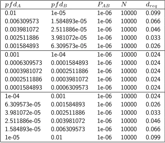
Tables 4, 5, 6 show examples, continuing the example introduced in Section 1. As before, the system pfd requirement is 10-6

, and the channel pfds have been chosen in each row of each table to give a product of 10-7

in the spirit of “conservatism about channel claims”. In the first column of each table, the successive values of pfdA from the top are 10-2

, 102.2 , 10-2.4

, … , 10-5

starting from the bottom, so that for each row pfdA×pfdB =10

−7

. The three tables differ in the number, N, of failure-free demands observed.

The tables show clearly the way in which asymmetry in the channel pfds aids the assessment: the more asymmetric these are, all things being equal, the greater the prior doubt about NWTI can be, whilst still allowing the claim about the system pfd. Thus in Table 4, the greatest doubt that can be allowed occurs when pfdA=10-2

, pfdB=10

-5 _{(or vice-versa). Similar results apply in Tables 5 and 6 although, for these} larger values of N, the differences between the largest allowable doubt and the smallest, over the range of values of the channel pfds, is less pronounced.

Notice that the value of dreq for large values of N, (15), depends on the channel probabilities of failure on demand, pfdA and pfdB, only via their product. The extent to which this product is smaller than PAB can be thought of as representing the degree of conservatism in the system pfd claim, compared with an over-optimistic claim of certain independence of channel failures. This is similar to the informal reasoning we reported in Section 1, but in our more formal treatment, the system claim is guaranteed to be conservative (for the assessor’s particular level of doubt about NWTI).

In Table 4, the central rows all have dreq=0.024. That is because for these values of the channel pfds, N=10000 is sufficiently large to satisfy (14) – i.e. zm is smaller than each channel pfd – and so in (15) dreq depends on the individual channel pfds only via their product, which is 10-7 _{in each row. This effect is even more pronounced in Tables 5} and 6, in which N is larger.

Examples 4

pf dA pf dB PAB N dreq

0.01 1e-05 1e-06 10000 0.099

0.006309573 1.584893e-05 1e-06 10000 0.066

0.003981072 2.511886e-05 1e-06 10000 0.046

0.002511886 3.981072e-05 1e-06 10000 0.033

0.001584893 6.309573e-05 1e-06 10000 0.026

0.001 1e-04 1e-06 10000 0.024

0.0006309573 0.0001584893 1e-06 10000 0.024

0.0003981072 0.0002511886 1e-06 10000 0.024

0.0002511886 0.0003981072 1e-06 10000 0.024

0.0001584893 0.0006309573 1e-06 10000 0.024

1e-04 0.001 1e-06 10000 0.024

6.309573e-05 0.001584893 1e-06 10000 0.026

3.981072e-05 0.002511886 1e-06 10000 0.033

2.511886e-05 0.003981072 1e-06 10000 0.046

1.584893e-05 0.006309573 1e-06 10000 0.066

1e-05 0.01 1e-06 10000 0.099

AP, DISPO mtng, 29/02/12 updt 20/04/12, slide 15of 21 Table 4: Values of dreq, i.e. prior doubt about NWTI, that must not be exceeded in order to support a system pfd claim of 10-6 _{after seeing 10,000 failure-free demands, for different values}

of the channel pfds (where, in each case, the product of the channel pfds is 10-7_{). Here}

[image:13.595.111.385.443.679.2]

Examples 5

pf dA pf dB PAB N dreq

0.01 1e-05 1e-06 50000 0.141

0.006309573 1.584893e-05 1e-06 50000 0.118 0.003981072 2.511886e-05 1e-06 50000 0.113 0.002511886 3.981072e-05 1e-06 50000 0.113 0.001584893 6.309573e-05 1e-06 50000 0.113

0.001 1e-04 1e-06 50000 0.113

0.0006309573 0.0001584893 1e-06 50000 0.113 0.0003981072 0.0002511886 1e-06 50000 0.113 0.0002511886 0.0003981072 1e-06 50000 0.113 0.0001584893 0.0006309573 1e-06 50000 0.113

1e-04 0.001 1e-06 50000 0.113

6.309573e-05 0.001584893 1e-06 50000 0.113 3.981072e-05 0.002511886 1e-06 50000 0.113 2.511886e-05 0.003981072 1e-06 50000 0.113 1.584893e-05 0.006309573 1e-06 50000 0.118

1e-05 0.01 1e-06 50000 0.141

[image:14.595.108.387.113.354.2]

AP, DISPO mtng, 29/02/12 updt 20/04/12, slide 17of 21

Table 5: As Table 4, but N=50,000, and zm=2.1e-05.

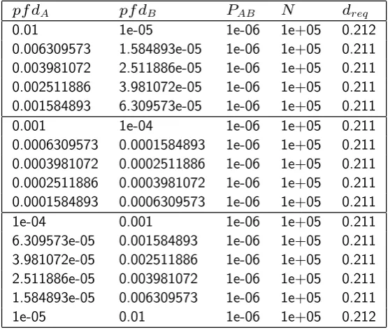
Examples 6

pf dA pf dB PAB N dreq

0.01 1e-05 1e-06 1e+05 0.212

0.006309573 1.584893e-05 1e-06 1e+05 0.211 0.003981072 2.511886e-05 1e-06 1e+05 0.211 0.002511886 3.981072e-05 1e-06 1e+05 0.211 0.001584893 6.309573e-05 1e-06 1e+05 0.211

0.001 1e-04 1e-06 1e+05 0.211

0.0006309573 0.0001584893 1e-06 1e+05 0.211 0.0003981072 0.0002511886 1e-06 1e+05 0.211 0.0002511886 0.0003981072 1e-06 1e+05 0.211 0.0001584893 0.0006309573 1e-06 1e+05 0.211

1e-04 0.001 1e-06 1e+05 0.211

6.309573e-05 0.001584893 1e-06 1e+05 0.211 3.981072e-05 0.002511886 1e-06 1e+05 0.211 2.511886e-05 0.003981072 1e-06 1e+05 0.211 1.584893e-05 0.006309573 1e-06 1e+05 0.211

1e-05 0.01 1e-06 1e+05 0.212

AP, DISPO mtng, 29/02/12 updt 20/04/12, slide 19of 21

Table 6: As Table 4, but N=100,000 and zm=1.1e-05.

[image:14.595.108.386.422.658.2]

– acceptable doubt is a factor of four greater than that where the channel pfds are approximately equal in size.

In Table 6, in contrast, N is sufficiently large that for almost all values of the channel pfds it is greater than NC and so dreq takes the same value in almost all cases. That is, channel asymmetry cannot be exploited here to increase allowable doubt in NWTI. Or, putting it more positively, for such large N there is no need to have one channel very much more reliable than the other to gain benefit in the size of dreq.

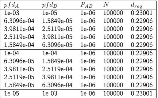
Tables 7, 8, 9 show similar results in a case where there is greater conservatism in the channel pfd claims: here the product is 10-8

in contrast to the 10-7

of the previous tables.

Examples 4.2.1

pf dA pf dB PAB N dreq

1e-03 1e-05 1e-06 10000 0.10838 6.3096e-04 1.5849e-05 1e-06 10000 0.072454 3.9811e-04 2.5119e-05 1e-06 10000 0.050118 2.5119e-04 3.9811e-05 1e-06 10000 0.036589 1.5849e-04 6.3096e-05 1e-06 10000 0.02909 1e-04 1e-04 1e-06 10000 0.026462 6.3096e-05 1.5849e-04 1e-06 10000 0.02909 3.9811e-05 2.5119e-04 1e-06 10000 0.036589 2.5119e-05 3.9811e-04 1e-06 10000 0.050118 1.5849e-05 6.3096e-04 1e-06 10000 0.072454 1e-05 1e-03 1e-06 10000 0.10838

[image:15.595.108.364.500.664.2]

AP, DISPO mtng, 29/02/12 updt 25/04/12, slide 18of 27

Table 7: Similar to Table 4, but with the channel pfds in each row having a product of 10-8_{, i.e.}

there is greater conservatism in the channel pfd claims.

Examples 5.2.1

pf dA pf dB PAB N dreq

1e-03 1e-05 1e-06 50000 0.15345

6.3096e-04 1.5849e-05 1e-06 50000 0.12831 3.9811e-04 2.5119e-05 1e-06 50000 0.12387 2.5119e-04 3.9811e-05 1e-06 50000 0.12387 1.5849e-04 6.3096e-05 1e-06 50000 0.12387

1e-04 1e-04 1e-06 50000 0.12387

6.3096e-05 1.5849e-04 1e-06 50000 0.12387 3.9811e-05 2.5119e-04 1e-06 50000 0.12387 2.5119e-05 3.9811e-04 1e-06 50000 0.12387 1.5849e-05 6.3096e-04 1e-06 50000 0.12831

1e-05 1e-03 1e-06 50000 0.15345

AP, DISPO mtng, 29/02/12 updt 25/04/12, slide 22of 27

Examples 6.2.1

pf dA pf dB PAB N dreq

1e-03 1e-05 1e-06 100000 0.23001 6.3096e-04 1.5849e-05 1e-06 100000 0.22906 3.9811e-04 2.5119e-05 1e-06 100000 0.22906 2.5119e-04 3.9811e-05 1e-06 100000 0.22906 1.5849e-04 6.3096e-05 1e-06 100000 0.22906 1e-04 1e-04 1e-06 100000 0.22906 6.3096e-05 1.5849e-04 1e-06 100000 0.22906 3.9811e-05 2.5119e-04 1e-06 100000 0.22906 2.5119e-05 3.9811e-04 1e-06 100000 0.22906 1.5849e-05 6.3096e-04 1e-06 100000 0.22906 1e-05 1e-03 1e-06 100000 0.23001

[image:16.595.108.366.94.254.2]

AP, DISPO mtng, 29/02/12 updt 25/04/12, slide 26of 27

Table 9: As Table 7, but with N=100,000.

3.1 Some observations arising from these examples

From a practical viewpoint an important question is how best to build (and test) a system so that the resulting dreq is larger than D. It seems that asymmetry of the channel pfds might be helpful here. However, since this essentially means that one of the channel pfds needs to be close to the required system pfd, it may not be a practical proposition in cases where very high system reliability is needed. In fact, such asymmetry goes against the spirit of this kind of fault tolerance, which is to build highly reliable systems from channels of only modest reliability.

The other factors affecting dreq are the conservatism of the system pfd claim (i.e. how much it differs from the too-optimistic simple product of the channel pfds), and the number of (failure-free) test cases observed. A comparison between Tables 4-6 and Tables 7-9 indicates the advantage, in terms of larger dreq, when there is greater conservatism (i.e. when the product of the channel pfds is 10-8

rather than 10-7 ).

Table 10 summarises the interplay between the product pfd_A×pfd_B, N and dreq: different levels of conservatism (pfd_A×pfd_B= 10-7_{, 10}-7.5_{, 10}-8_{), to support the same} system pfd claim of 10-6

, are shown against their corresponding values of the doubt in NWTI needed for different values of N.

[image:17.595.146.441.92.285.2]

pfdA×pfdB PAB N dreq 1e-7.0 1e-7.5 1e-8.0 1e-6 1e-6 1e-6 10000 10000 10000 0.099 0.106 0.108 1e-7.0 1e-7.5 1e-8.0 1e-6 1e-6 1e-6 50000 50000 50000 0.141 0.15 0.153 1e-7.0 1e-7.5 1e-8.0 1e-6 1e-6 1e-6 100000 100000 100000 0.212 0.225 0.230

Table 10: Upper bounds on the prior doubt about NWTI required to support a system pfd claim of 10-6_{, for three different values of pfd}

A.pfdB, for three different values of N.

Of course, such questions can really only be answered when there is specific evidence available about a particular system. However, we believe – somewhat tentatively – that it is reasonable to answer in the affirmative in some of the cases above. Take Table 9. Here there is considerable conservatism in the channel claims (product equals 10-8

versus a system claim of 10-6

), so that an assessor’s doubt about NWTI can be as high as 23% and still allow him to accept the system claim. He can do this without appealing to channel asymmetry (i.e. an implausibly strong claim for one of the channels), because the middle row of the table shows that claims of 10-4

for each channel will be sufficient. Such claims seem relatively modest for channels that have been built to safety-critical standards: for example, they could be supported by feasible amounts of operational testing. The number of system test cases (100000) that need to be generated is large, of course. Whether this is feasible will depend on particular circumstances, but we note that for a real protection system it is proposed to generate 50000 test cases (HSE 2011). Notice, however, that even 100000 test cases is more than an order of magnitude fewer than would be needed to support the system pfd claim of 10-6

directly from a “black-box” test (Littlewood and Wright 1997).

4

Discussion

We have presented a new way of reasoning about the reliability of a 2-channel, 1-out-of-2 software-based system that overcomes some of the objections that can be made about an earlier approach to the problem. This earlier approach can be characterized as follows: “We realize that an assumption of independence between failures (and thus a claim for system pfd that is the simple product of channel pfds) may be too optimistic, but we have compensated for that by making only very conservative claims for the channel pfds. The system pfd claim will thus be conservative.”

parameters (prior doubt about NWTI, number of failure-free tests observed, product of channel pfds, system pfd claim). However, the attentive reader will have noticed that this new approach brings its own problems and some difficulties that need further thought.

In the first place, we have assumed in the development of Section 2 that the channel probabilities of failure on demand, pfdA and pfdB, are known. In practice, of course, these probabilities will not be known with certainty. One way forward would be to use the ideas in (Bishop, Bloomfield et al. 2011), where it was shown how to obtain a conservative bound for the posterior mean of the pfd of a single system based on an assessor’s prior belief and the observation of some failure-free demands in statistically representative operational testing. Such bounds could be used by an assessor as if they were “true” pfds, in the knowledge that they will be conservative. The testing of the different channels to obtain these pfds would be carried out before the system testing required for the results of Sections 2 and 3. In the current model there is no further “learning” about these channel pfds from the system testing. That is, the likelihood function used in the Bayesian updating in Section 2 does not allow any updating of the assessor’s knowledge of his beliefs about the channel pfds. The evidence from the system testing is just that there have been no system failures in N tests, but the assessor does not know whether there have been individual channel failures. Informally, the Bayesian updating in Section 2 concerns only the channel failure dependence via the evolution of dAB(N) and zAB(N) as N increases, but not any evolution of the channel reliabilities.

This may be realistic in some cases: for example, in the case of shut-down systems, when a preferred channel correctly causes shut-down, the other channel may not be invoked and so it may not be known if it would have failed to shut down on that demand. However, in many cases this view will be too restrictive, and the system tests will also give information about channel outcomes. In such cases it would be useful to extend the model to be able to take account of this information: this is an issue we plan to address in future work. In fact such an extended model may also allow greater confidence to be gained in NWTI: informally, seeing some single channel failures, but no system failures, may give greater confidence in the efficacy of the fault tolerance mechanism (albeit less confidence in the reliabilities of the channels). A major difficulty in this model, of course, centres upon the assessor’s prior doubt about no-worse-than-independence of channel failures. Is it reasonable to expect an assessor to be able to state a numeric value for D, and for this number to be genuinely meaningful, rather than simply an uninformed guess? Interestingly, in private discussions with safety engineers and regulators familiar with these kinds of multi-channel systems we have found a willingness to express numerically their confidence about independence itself: e.g. “I am 90% confident that failures of these channels will be independent”. In supporting such claims the experts usually appeal to their detailed knowledge of the architectures of the target systems, and on how they were built.

design and build processes. Using such evidence to support probabilistic measures of doubt, as is required here, may not be easy.

Because of these difficulties, we think that the most plausible use for our work might lie in providing challenges to claims based upon the kind of informal “trade-off” arguments we criticized in Section 1. Such a challenge might be of the following form: “You say that your channel pfd claims are pessimistic by these amounts, and that you have seen this number of representative failure-free test cases, it follows that, to support your system pfd claim, your doubt in NWTI needs to be smaller than this number.” That is, our work can be seen as a way of ‘policing’ assessor claims by revealing what is needed to be believed in order to support a system claim: such required beliefs may be unreasonable in the view of, say, a nuclear regulator, and thus open the claim to rejection.

Of course, it would help to have empirical evidence of the levels of dependence between diverse software-based channels in some real-life systems. Unfortunately, such evidence is very thin on the ground. However, a single data point comes from the multi-version experiment conducted by Knight and Leveson (Knight and Leveson 1986). There the null hypothesis of NWTI was not rejected for 139 out of 162 pairs of versions. That is, the estimated doubt in NWTI for a randomly selected pair was 0.142 (Povyakalo and Littlewood 2010) which compares favourably with the 0.23 doubt in the discussion of the previous section. It has to be said, though, that the problem addressed here was not comparable to a real safety-critical application, such as a protection system, and the versions were not developed under the kind of conditions that might be expected of such applications.

Ideally, we would like to have empirical evidence of the channel dependencies achieved in real systems. We are not aware of such evidence being available currently, in spite of several well-known multi-channel software-based systems having received extensive operational exposure. What is needed is that channel “vote-outs” be recorded in those situations where there is no system failure (as well as when there is system failure, of course). We are not aware that this is done as a matter of course in any existing systems, and have seen no published data of this kind.

Even if such data were available, across many disparate safety-critical systems in operation, there would be difficulties in an assessor using them to make a judgment about his confidence in NWTI for a particular novel system, since this new one may differ in significant ways from the previous ones.

However, in some industries, there may be considerable experience in building “similar” systems in the past: e.g. protection systems. Let us assume that these earlier systems have been successful, in the sense that they were accepted as sufficiently safe to be deployed, and these judgments were not overruled by operational experience. An assessor could retrospectively compute dreq for each of these previous systems. It might then be conservative for him to use, say, the smallest of these numbers as his prior doubt, D, for a novel system. Such a choice could be regarded as ensuring that the procedure for assuring the safety of a new system was no worse – i.e. no less stringent – than that adopted historically.

Acknowledgements

dealt with in this paper: Bob Jennings and Bob Yates from Office of Nuclear Regulation; Silke Kuball from EDF; Peter Bishop, Lorenzo Strigini and Robin Bloomfield from CSR. We also thank the Associate Editor and three reviewers for extensive and helpful comments on an earlier version of the paper.

Support for the work reported here came from:

• the UnCoDe project, funded by the Leverhulme Trust;

• The DISPO project - funded under the C&I Nuclear Industry Forum (CINIF) Nuclear Research Programme by EDF Energy Limited, Nuclear Decommissioning Authority (Sellafield Ltd, Magnox Ltd), AWE plc, Urenco UK Ltd and Horizon Nuclear Power. The views expressed in this paper are those of the authors and do not necessarily represent the views of CINIF members. CINIF does not accept liability for any damage or loss incurred as a result of the information contained in this paper.

References

Bishop, P., R. Bloomfield, et al. (2011). "Towards a formalism for conservative claims about the dependability of software-based systems." IEEE Trans Software Engineering 37(5): 708-717.

Bloomfield, R. and B. Littlewood (2003). Multi-legged arguments: the impact of diversity upon confidence in dependability arguments. International Conference on Dependable Systems and Networks (DSN2003), San Francisco.

Eckhardt, D. E., A. K. Caglayan, et al. (1991). "An experimental evaluation of software redundancy as a strategy for improving reliability." IEEE Trans Software Eng 17(7): 692-702.

Eckhardt, D. E. and L. D. Lee (1985). "A Theoretical Basis of Multiversion Software Subject to Coincident Errors." IEEE Trans. on Software Engineering 11: 1511-1517.

HSE (2011). Step 4 Control and Instrumentation Assessment of the EDF and AREVA UK EPR Reactor. Bootle, Health and Safety Executive, Office for Nuclear Regulation.

Knight, J. C. and N. G. Leveson (1986). An Empirical Study of Failure Probabilities in Multi-version Software. Proc. 16th Int. Symp. on Fault-Tolerant Computing (FTCS-16), Vienna, Austria.

Knight, J. C. and N. G. Leveson (1986). "Experimental evaluation of the assumption of independence in multiversion software." IEEE Trans Software Engineering 12(1): 96-109.

Littlewood, B. and D. R. Miller (1989). "Conceptual Modelling of Coincident Failures in Multi-Version Software." IEEE Trans on Software Engineering 15(12): 1596-1614.

Littlewood, B. and L. Strigini (2000). A discussion of practices for enhancing diversity in software designs. London, Centre for Software Reliability, City University: 58.

Littlewood, B. and D. Wright (1997). "Some conservative stopping rules for the operational testing of safety-critical software." IEEE Trans Software Engineering 23(11): 673-683.

May, J., G. Hughes, et al. (1995). "Reliability estimation from appropriate testing of plant protection software." Software Engineering Journal 10(6): 206-218. Povyakalo, A. and B. Littlewood (2010). Probably independent random variables and

conservative bounds for expectation of their product. London, Center for Software Reliability, City University.

Finding a worst case prior distribution

Statement

Let P be the system pfd treated as a random variable with density f(p), where 0pz01.

Here we show that

E(P |N failure free demands) =

1 Rz0

0_R (1 p)N+1f(p)dp

z0

0 (1 p)Nf(p)dp 

1 (1 p1)

N+1_{(1 x) + (1 p}

2)N+1x

(1 p1)N_{(1 x) + (1 p2)}N_x (A1)

where

0p1 yp2z0 (A2)

Z y

0 f(p)dp= 1 x.

and the bound (A1) is reached with the two-point prior probability distri-bution ofP:

P rob(P =p1) = 1 x; P rob(P =p2) =x;

Lemma

Ifq is a positive random variable and N is a positive integer, then

[E(qN+1)]N1+1 _[E(qN_)]N1

Proof Ifx 0 anda 1 the functionf(x) =xais convex, so, by Jensen’s inequality

E(xa) (E(x))a (A3)

Substituting x=qN and a= N_n+1 into (A3):

E(qN+1) [E(qN)]NN+1

which implies

[E(qN+1)]N1+1 [E(qN)]N1

QED

p1 = 1 Ry

0(1 p)N+1f(p)dp

1 x

! 1

N+1

p2 = 1

Rz0

y (1 p)N+1f(p)dp

x

! 1

N+1

p3 = 1 Ry

0(1 p)Nf(p)dp

1 x

!1

N

p4 = 1

Rz0

y (1 p)Nf(p)dp

x

!1

N

Obviously,

0_p1, p3 y

y_p2, p4 z0

In accordance with the lemma

p1p3 (A4)

p2p4 (A5)

because

1 p1= (E((1 P)N+1|P y)) 1

N+1

1 p3= (E((1 P)N |P y)) 1

N

1 p2= (E((1 P)N+1|P > y)) 1

N+1

1 p4= (E((1 P)N |P > y)) 1

N

We can now use the values p1, p2, p3, p4 to write down an expression for

E(P |N successful runs)

E(P _|N successful runs) =

1

Rz0

0_R (1 p)N+1f(p)dp

z0

0 (1 p)Nf(p)dp

= (A6)

1

Ry

0(1 p)N+1f(p)dp+ Rz0

y (1 p)N+1f(p)dp

Ry

0(1 p)Nf(p)dp+ Rz0

y (1 p)Nf(p)dp

=

1 (1 p1)

N+1_{(1 x) + (1 p}

2)N+1x

(1 p3)N(1 x) + (1 p4)Nx

E(P |nsuccessful runs)

1 (1 p1)

N+1_{(1 x) + (1 p}

2)N+1x (1 p1)N(1 x) + (1 p2)Nx

(A7)

and the bound (A7) is obviously reached when one chooses the two-point prior distribution of P:

P rob(P =p1) = 1 x;

P rob(P =p2) =x; 0_p1 yp2 z0 1.

QED

Finding p1 and p2

The unknown values p1 and p2 are found as a solution of two-dimensional optimisation problem

F(p1, p2) = (1 p1)

N+1_{(1 x) + (1 p2)}N+1_x (1 p1)N(1 x) + (1 p2)Nx !

min

subject to constraints:

0_p1 y;

y_p2 z0.

In general, p1 and p2 may di↵er fromy and z0. However,

@F

@p1

= (1 p1)N 1(1 x)⇥

(1 p1)N+1(1 x) + (N(p2 p1) + 1 p1)(1 p2)Nx ((1 p1)N(1 x) + (1 p2)Nx)2 

0,

because (A2) impliesp1p2.

Thus,F(p1, p2) reaches its minimum when p1 =y.

Using the following substitution, we obtain the result in the main body of the paper for a ”1-out-of-2” system with knownpf dA,pf dBandP(pf dAB >

pf dApf dB) =dAB(0),

p1 =y=pf dA·pf dB;

p2 =zAB(N);

z0= min(pf dA, pf dB);

x=dAB(0).

Here, we aim at finding the required prior doubtdreq, satisfying

PAB = 1

(1 dreq)(1 pf dA·pf dB)N+1+dreq(1 z)N+1 (1 dreq)(1 pf dA·pf dB)N+dreq(1 z)N

, (A8)

where

pf dA·pf dB zmin(pf dA, pf dB) (A9)

and zminimises function FAB(u):

FAB(u) =

(1 dreq)(1 pf dA·pf dB)N+1+dreq(1 u)N+1 (1 dreq)(1 pf dA·pf dB)N+dreq(1 u)N

,

given the parametersPAB,pf dA,pf dB and N are known.

Notation

Let us denote

z0= min(pf dA, pf dB) (A10)

y=pf dA·pf dB (A11)

E(z) = (1 dreq)(1 y)N+1+dreq(1 z)N+1 D(z) = (1 dreq)(1 y)N +dreq(1 z)N

FAB(z) = E(z) D(z)

(A12)

Finding z

In order to findz, we need the following derivatives and function G:

E0(z) = (N+ 1)_·dreq·(1 z)N D0(z) = N ·dreq·(1 z)N 1

G(z) =E0(z) D0(z)FAB(z) = (A13)

((N+ 1)(1 z) +N FAB(z))(1 z)N 1;

F_AB0 (z) = E0(z)D(z) E(z)D0(z)

D(z)2 =

G(z)

D(z) (A14)

Thus, in accordance with (A13) and (A14), every stationary pointz0 of FAB(z) satisfies the equation

(N+ 1)(1 z0) N FAB(z0) = 0.

z0= 1

✓

1 1

N+ 1

◆

(1 PAB)z0. (A15)

Otherwise, if, z0 > z0, then

(N+ 1)(1 z0) N(1 PAB) 0, (A16)

andFAB(z) reaches the required minimum 1 PAB at the endz=z0 of the segment [y, z0] , becauseFAB(y) = 1 y PAB.

Therefore,

z= min(z0, z0). (A17)

Inequality (A16) can be re-written as following

N _ 1 z0 z0 PAB

. (A18)

Finding dreq

Now, let’s denote

w= 1 dreq

dreq

= 1

dreq 1,

re-write (A8) as following

1 PAB =

w(1 pf dA·pf dB)N+1+ (1 z)N+1

w(1 pf dA·pf dB)N+ (1 z)N

,

and solve it with respect tow

w= z PAB

PAB y

✓_{1 z}

1 y

◆N

,

Thus, finally

dreq=

1

1 +z PAB

PAB y ⇣

1 z 1 y

⌘N,

because

dreq= 1 1 +w

N  1 min(pf dA, pf dB) min(pf dA, pf dB) PAB

,

thenz=z0= min(pf dA, pf dB) and

dreq= 1

1 +min(pf dA,pf dB) PAB

PAB pf dA·pf dB

⇣_{1 min(pf d}

A,pf dB)

1 pf dA·pf dB

⌘N.

If

N > 1 min(pf dA, pf dB) min(pf dA, pf dB) PAB

,

thenz=z0

dreq =

1

1 +z0 PAB

PAB y

⇣

1 z0

1 y

⌘N. (A19)

Equality (A17) implies

1 z0 =

✓

1 1

N + 1

◆

(1 PAB) =

✓

1 + 1 N

◆ 1

(1 PAB). (A20)

and

z0 PAB = (1 PAB) (1 z0) = (1 PAB) 1

N + 1. (A21) Substituting (A11),(A20) and (A21) into (A19), we finally get

dreq=

1

1 + 1 PAB

PAB pf dA·pf dB

⇣ _{1 P}

AB

1 pf dA·pf dB

⌘N⇣

1 +_N1⌘ N _N1₊₁ .

Summary

Thus, we have shown that:

1. If

N  1 min(pf dA, pf dB) min(pf dA, pf dB) PAB

,

then

dreq = 1

1 +min(pf dA,pf dB) PAB

PAB pf dA·pf dB

⇣_{1 min(pf d}

A,pf dB)

1 pf dA·pf dB

⌘N.

2. If

N > 1 min(pf dA, pf dB) min(pf dA, pf dB) PAB

,

then

dreq=

1

1 + 1 PAB

PAB pf dA·pf dB

⇣ _{1 P}

AB

1 pf dA·pf dB

⌘N⇣

1 +_N1⌘ N _N1₊₁ .

problems associated with the dependability of software-based systems, and has published many papers in international journals and conference proceedings and has edited several books. His technical contributions have largely focused on the application of rigorous probabilistic and statistical techniques in software

systems engineering. In 1983 he founded the Centre for

Software Reliability (CSR) at City University, London, and was its Director until 2003. He is currently

Professor of Software Engineering in CSR. From 1990 to 2005 he was a member of the UK Nuclear Safety

Advisory Committee. He is a member of IFIP Working

Group 10.4 on Reliable Computing and Fault Tolerance, of the UK Computing Research Committee, and is a Fellow of the Royal Statistical Society. He is on the editorial boards of several international journals. In

2007 he was the recipient of the IEEE Computer Society's Harlan D Mills Award.

Andrey Povyakalo has MSc equivalent degree in

computer-aided control and management from the

Moscow State Institute for Physics and Engineering

(MIPHE, 1985) and PhD equivalent degree in

mathematical modelling in nuclear engineering from the

Institute of Nuclear Power Engineering, Obninsk,

Russia (INPE, 1994). In 1985-2001 he worked for INPE

as lecturer, senior lecturer and associate professor

contributing to a number of research projects related to

probabilistic safety analysis and risk assessment (PSA/PRA). In 2001 Andrey joined the Centre for

Software Reliability (CSR), City University, London as a research fellow working for the interdisciplinary

research collaboration on dependability of computer-based systems (DIRC, 2000-2006) funded by the UK Engineering and Physical Science Research Council (EPSRC). In 2005 (in co-authorship with E. Alberdi, L. Strigini and P. Ayton) he was a recipient of the 2005 Herbert M. Stauffer Award for the "Best Clinical Paper" from the Association of University Radiologists. At

present, he is a senior lecturer in dependability of socio

-technical systems. His research interests are mostly

related to probabilistic modeling of confidence in