Common mortality modelling and coherent forecasts. An empirical analysis of worldwide mortality data

      

City, University of London Institutional Repository

Citation

:

Hatzopoulos, P. & Haberman, S. (2013). Common mortality modelling and coherent forecasts. An empirical analysis of worldwide mortality data. Insurance:

Mathematics and Economics, 52(2), pp. 320-337. doi: 10.1016/j.insmatheco.2013.10.009

This is the accepted version of the paper.

This version of the publication may differ from the final published

version.

Permanent repository link:

http://openaccess.city.ac.uk/15995/

Link to published version

:

http://dx.doi.org/10.1016/j.insmatheco.2013.10.009

Copyright and reuse:

City Research Online aims to make research

outputs of City, University of London available to a wider audience.

Copyright and Moral Rights remain with the author(s) and/or copyright

holders. URLs from City Research Online may be freely distributed and

linked to.

City Research Online: http://openaccess.city.ac.uk/ publications@city.ac.uk

Common mortality modelling and coherent forecasts. An empirical analysis of

worldwide mortality data

P. Hatzopoulos

a

, S. Haberman

b

a

Department of Statistics and Actuarial-Financial Mathematics, University of the Aegean, Samos, 83200, Greece b

Faculty of Actuarial Science and Insurance, Sir John Cass Business School, City University, 106 Bunhill Row, London EC1Y8TZ, UK

Abstract

A new common mortality modeling structure is presented for analyzing mortality dynamics for a pool of countries, under the framework of generalized linear models (GLM). The countries are first classified by fuzzy c-means cluster analysis in order to construct the common sparse age-period model structure for the mortality experience. Next, we propose a method to create the common sex difference age-period model structure and then use this to produce the residual age-period model structure for each country and sex. The time related principal components are extrapolated using dynamic linear regression (DLR) models and coherent mortality forecasts are investigated. We make use of mortality data from the “Human Mortality Database”.

Keywords: Fuzzy c-Means Cluster; Generalized Linear Models; Sparse Principal Component Analysis; Dynamic Linear Regression; Mortality Forecasting; Residuals; Coherent;

1. Introduction

The remainder of the paper is organised as follows. In section 2, utilizing mortality data from the “Human Mortality Database, we group 35 countries using fuzzy c-means cluster analysis. In this way, we form the West-cluster and East-West-cluster countries, for both sexes, and we construct the common age-time mortality dynamics, using 19 males West-cluster countries. Next, we employ Sparse Principal Component Analysis (SPCA) to these common mortality rates, in order to derive the common age-period model structure, for both sexes. In section 3, we construct the sex difference mortality dynamics, and compare the mortality experience of males and females. In section 4, we analyze the residual particularities for each country, based on the common age-period model for males, and the common age-period and sex difference model structure for females. In section 5, we utilize dynamic linear regression (DLR) model structures, to implement coherent forecasts. Finally, in section 6, we discuss the results and offer some concluding comments.

2. Common age-period mortality dynamics

Initially, we need to choose which countries will be selected to describe the common patterns of mortality dynamics. We require the pooled countries to contain similar characteristics. Cluster analysis is a reasonable approach to separate the countries into clusters with similar mortality dynamics. Data clustering is the process of dividing data elements into classes or clusters so that items in the same class are as similar as possible, and items in different classes are as dissimilar as possible.

Following Hatzopoulos and Haberman (2009)), the log-graduated central mortality rates, in age-period effects, can be decomposed as an age-period association model structure (see model 2, Hatzopoulos and Haberman (2009)). According to this model structure, the main time effects component, values, is an index of the level of mortality that captures the overall time trend at all ages, and summarizes the overall mortality dynamics across time. Also, the main time trends are independent of the level of mortality (a zero centred vector, constructed by linear combinations of principal component scores). Therefore, we could base our cluster analysis on these main time trends. In classic cluster analysis, the data are divided into distinct clusters, where each data element belongs to exactly one cluster. Alternatively, in fuzzy clustering, data elements can belong to more than one cluster, each associated with a membership level. This indicates the strength of the association between that data element and a particular cluster. Utilizing Fuzzy C-Means cluster analysis on the main time effects, for each country, we can distinguish the similarities or the dissimilarities among the countries. One of the most widely used fuzzy clustering algorithms is the Fuzzy C-Means (FCM) Algorithm. This technique was originally introduced by Jim Bezdek as an improvement on earlier clustering methods (Bezdek, 1981). The FCM algorithm attempts to partition a finite collection of c elements

( )

b t

1, 2,..., c

X = X X X into a collection of f fuzzy clusters. The algorithm returns a list of f cluster multidimensional centres

C

C C

₁

,

₂

,...,

C

_f

ij

u

=

, and a

partition matrix of membership grades [0, 1], i=1, . . .,c, j=1, . . .,f, where each element tells the degree to which element

ij

U

=

u

∈

i

X belongs to cluster

C

_j.

We utilise the mortality data from the “Human Mortality Database” (HMD) (www.mortality.org). The bulk of countries (35 countries), from the HMD, have a common time range 1960-2006, and hence we apply the FCM algorithm to those national mortality data. Experiments with different numbers of clusters, gives a distinctive separation with f=2 clusters. In Table 1, the columns give the optimum number of GLM parameters for the graduated (or full) model structure, according to the Bayesian Information Criterion (BIC) (see Hatzopoulos and Haberman (2009) equation 2.1). The

r

k

r

μ

-values are the overall means for each country, according to the age-period association model structure, and equal to the average value of the logged central rates of mortality across age and time. The -values, give the fuzzy c-means membership levels for the first cluster (the membership value for the second cluster is complementary to the first one).

1

i

u

According to the -values, in Table 1, we form the males and females first cluster countries, which consists of 25 countries and 26 countries respectively. The common countries that belong to the first cluster, for both sexes, are the following 24 countries: Sweden, France, Denmark, E&W (England & Wales), Norway, Netherlands, Scotland, Italy, Switzerland, West Germany, Finland, Spain, Ireland, Belgium, Austria, Portugal, Luxembourg, Australia, New Zealand, Canada, USA, Japan, Czech and East Germany. The countries are sorted in decreasing

1

i

manner according to their fuzzy c-means -membership levels. White (2002) has observed that a group of 17 countries with a real GNP per capita of at least half that of the United States in 1970 and continuously democratic government, show strong convergence on life expectancies, for the period 1955-96. The countries involved are: Australia, Austria, Belgium, Canada, Denmark, Finland, France, West Germany, Italy, Japan, Netherlands, New Zealand, Norway, Sweden, Switzerland, United Kingdom and USA. We note that all of these 17 countries belong to the first West-cluster (Table 1, values). Also, Wilson (2001), using data from the World Population Prospects (United Nations 1999), has discussed the fundamental differences in the respective histories of the First, Second, and Third Worlds over the last 50 years which justify the trichotomy: developed, developing and former Communist states of the Soviet Union and Eastern Europe. In that assessment, “former Communist” is defined as the Soviet Union and all European countries ruled by Communist parties in the Cold War era, and the “developed” category includes the other European countries, along with the United States, Canada, Australia, New Zealand, and Japan, and “developing” is the rest of the world. In Table 1, all of the countries with large values belong to the “developed” countries, except for the Czech Republic and East Germany.

1

i

u

r

1

i

u

1

i

u

In addition, applying the FCM clustering algorithm to the remaining East-cluster countries (10 countries for males and 9 for females), gives another distinct pair of countries. The -values, in Table 1, give their fuzzy c-means membership levels for the first East sub-cluster. We observe distinct -values for the countries: Belarus, Ukraine and Russia, for both sexes, which form the first sub-cluster of the East-countries.

1

i

v

1

i

v

Males _kr

μ

_{ui1 vi1} Females

_k

_r

r

μ

u

i1 vi1

1 Sweden 16 -5.452 99% Canada 17 -5.859 99%

2 E&W 23 -5.318 99% Sweden 15 -5.986 98%

3 France 23 -5.152 99% Switzerland 15 -5.934 98%

4 Belgium 16 -5.773 98% France 17 -5.847 98%

5 Netherlands 16 -5.397 98% Belgium 16 -5.773 98%

6 Switzerland 16 -5.310 98% Australia 17 -5.844 96%

7 Canada 17 -5.266 98% Austria 16 -5.778 96%

8 New Zealand 16 -5.181 98% E&W 17 -5.837 95%

9 Portugal 16 -4.934 98% W.Germany 17 -5.787 95%

10 Italy 18 -5.284 97% Portugal 15 -5.584 95%

11 Norway 16 -5.335 96% Spain 17 -5.881 93%

12 Australia 17 -5.249 96% Italy 18 -5.901 92%

13 Spain 17 -5.249 96% Finland 15 -5.828 92%

14 W.Germany 23 -5.199 96% New Zealand 10 -5.714 90%

15 Austria 16 -5.127 96% E. Germany 16 -5.692 90%

16 USA 24 -5.071 96% Ireland 10 -5.764 88%

17 Finland 16 -5.068 96% Scotland 15 -5.677 83%

18 Luxembourg 9 -5.009 96% Netherlands 16 -5.921 82%

19 Iceland 9 -5.287 93% Japan 17 -5.930 80%

20 Scotland 16 -5.126 93% Luxembourg 8 -5.536 80%

21 Ireland 10 -5.204 89% Czech 16 -5.675 78%

22 E. Germany 16 -5.101 88% USA 24 -5.666 78%

23 Japan 24 -5.360 87% Denmark 11 -5.788 76%

24 Czech 16 -5.004 87% Poland 17 -5.629 73%

25 Denmark 16 -5.269 81% Norway 10 -5.973 70%

26 Poland 22 -4.908 44% 9% Slovakia 15 -5.634 60%

27 Slovakia 16 -4.935 42% 10% Hungary 16 -5.506 33% 13%

28 Hungary 16 -4.889 18% 5% Iceland 6 -5.742 15% 34%

29 Belarus 16 -4.730 7% 95% Russia 27 -5.280 12% 94%

30 Ukraine 19 -4.643 7% 98% Ukraine 20 -5.386 9% 98%

31 Russia 24 -4.445 7% 95% Belarus 16 -5.520 8% 95%

32 Estonia 10 -4.654 5% 20% Estonia 10 -5.486 7% 14%

33 Latvia 15 -4.604 4% 35% Bulgaria 16 -5.496 5% 15%

34 Bulgaria 16 -4.954 3% 31% Latvia 10 -5.429 5% 15%

35 Lithuania 15 -4.717 1% 56% Lithuania 14 -5.514 4% 6%

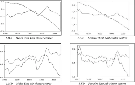
In panel 1.M.a of Figure 1, we display the fuzzy cluster centres,

(

C C

₁

,

₂

)

,

in time effects for the males West-cluster countries (graph with decreasing trend) and the males East-West-cluster countries (graph with relative steady trend). Panel 1.F.a, similarly displays the cluster centres for the females West-cluster countries (graph with decreasing trend) and the females East-cluster countries (graph with slight decreasing trend). In panels 1.M.b & 1.F.b, respectively, we display the cluster centres,

(

C C

1

,

2

)

,

for the two East sub-cluster countries for both

sexes. We note the change in the trend of the cluster centres after 1990s, for each East sub-cluster, for both sexes. The increasing trend, particularly after the 1990s, for males refers mainly to Belarus, Lithuania, Ukraine and Russia and for females refers to Belarus, Ukraine and Russia (with larger values

,

Table 1). For the remaining East-cluster countries, namely: Poland, Slovakia, Hungary, Estonia, Latvia and Bulgaria for males, and Hungary, Iceland, Estonia, Bulgaria, Latvia and Lithuania for females (with smaller values

,

Table 1), the decreasing trend is noticeable after the 1990s, for both sexes.

1

i

v

1

i

v

-0,5 -0,3 -0,1 0,1 0,3

1960 1970 1980 1990 2000

1.M.a Males West-East cluster centres 1.F.a Females West-East cluster centres

-0,3 -0,1 0,2

1960 1970 1980 1990 2000

[image:5.595.78.551.236.532.2]

1.M.b Males East sub-cluster centres 1.F.b Females East sub-cluster centres

Figure 1: Cluster centres in fuzzy c-means clustering. 1.M.a & 1.F.a graphs refer to all 35 countries, which form the West (graphs with decreasing trend) and East cluster countries, for males-females respectively. The 1.M.b & 1.F.b graphs refer to the sub-clusters of the East-cluster countries (the increasing trend, after the 1990s, refers mainly to Belarus, Ukraine and Russia), for males-females respectively.

Although we could employ the West-cluster mortality experience for the time period 1960-2006 for fitting the models, we need to refer to as long a mortality history as possible, in order to produce viable long term forecasts. Many authors begin their mortality analyses after the second half of the 20th century, effectively after the end of World War II, for modelling and forecast purposes. For example, Lee (2003) comments that the mortality age schedule has changed shape between the first and second halves of the 20th century. These results indicate that any forecasts would better be based on the post-war mortality experience, when mortality patterns have changed, in comparison with earlier periods of time, on the assumption that these dynamics will continue into the future. Therefore, we utilize the post-war mortality experience to construct common mortality trends, including all of those countries which belong to the West-cluster countries, and have available mortality data from the HMD since 1947. As a result, the countries included are the following 19 countries: Sweden, France, Denmark, E&W, Norway, Netherlands, Scotland, Italy, Switzerland, Finland, Spain, Ireland, Belgium, Australia, Canada, USA, Portugal, Japan and Austria.

)

modeling the age mortality effects is based on heteroscedastic Poisson error structures. In this context, the data for analysis, which are denoted by

(

d

_{x t r, ,}

,

R

_{x t r, ,} , comprise the observed number of deaths,

d

x t r, , , with

matching central exposures to the risk of death,

R

_{x t r, ,}

1

t

t

_n

, defined over rectangular data grids (x,t), with t ranging over the individual calendar years range [ , ] and x ranging over the age range [

x

₁,

x

_a], for each country . We model the response variates, the observed number of deaths as independent realizations of Poisson random variables,

1, ,...,2 c

r =r r r

, ,

x t r

D

, conditional on the central exposures

R

_{x t r, ,} , i.e.

, ,

(

,

( )

, ,

)

x t r

D

∼

Poiss

on m

x r

t

⋅

R

x t r (Brillinger, 1986), for each calendar year independently:

, , , , ,

(

x t r

)

x r

( )

x t r

E D

=

m

t

⋅

R

and

Var D

(

x t r_{, ,}

)

=

ϕ

t r_,

⋅

E D

(

x t r_{, ,}

)

where denotes the central rate of mortality, for each age, calendar year and country. The over-dispersed parameter is independent of the response variate, and is the theoretical equivalent of the empirical variance ratio r discussed by Forfar et al (1988) and can be estimated by the ratio of the quasi-deviance divided by the associated degrees of freedom.

,

( )

x r

m

t

, t r

ϕ

Under this approach, we need to construct pooled common number of deaths with matching central exposures in order to construct common central rates. We note that, if we were just to add up the actual number of deaths

from all the countries together, say

1 , ,. , , c r x t r r

d

d

=

=

∑

_{x t r}, treating them as independent realizations of Poisson

random variables,

D

x t, ,., conditional on the central exposures

1 , ,. , , c r x t r r

R

R

=

=

∑

x t r , i.e.

, ,.

(

ˆ

, ,.

)

x t

D

∼

Poisson D

_{x t} , for each calendar year independently, then the countries with the biggest populations

would dominate the overall mortality analysis. We need weighted deaths

d

x t rw, , , and matching weighted central

exposures

R

x t rw, , , such that, each country will contribute equivalent to the pooled common mortality experience.

Applying unweighted deaths, to the model structure proposed in this paper, results in reducing the coherent structure. We construct a set of weights under the assumption that, for each calendar year, the sum of the weighted deaths over all ages are equal for each country. For identification reasons, the sum of the weights, per calendar year, over all countries must sum up to the number of countries. The weights that satisfy the above two

constraints for each country and calendar year are given by

1 , ., , ., , 1 c

t r _r

t r t r r r c w d d = = _{⎡ ⎤} ⎢ _{⎥ ⋅} ⎢ ⎥ ⎢ ⎥ ⎣

∑

⎦ , where

denote the sum of deaths over all the ages, for each country and calendar year. The constructed weighted deaths are the product of the constructed weights and the observed deaths, i.e.

1

., , , ,

a

x

t r x t r

x x

d

d

=

=

∑

, , , , , w

x t r

=

t r

⋅

d

xt r

d

w

, with matching

weighted central exposures

R

x t rw, ,

=

w

t r,

⋅

R

x t r, , . In the specific situation, where the sum of deaths over all the

ages are equal for each country, then the weights are equal to one and the weighted deaths are equivalent to the observed deaths. We now model the weighted number of deaths,

d

x t rw, ,

,

as independent realizations of Poisson

random variables,

D

x t rw, , , conditional on the weighted central exposures

R

x t rw, , , i.e.

, , ,

w

, ,

)

w

)

(

(

x t r x r

D

∼

Poisson m

t

⋅

R

x t r , for each calendar year independently:

E D

(

x t rw, ,

)

=

m

x r,

( )

t

⋅

R

x t rw, , and

, , ,

(

_{x t r}w

)

_{t r}

(

w_{, ,}

)

Var D

=

ϕ

⋅

E

D

_{xt r} . Then, the sum of the independent Poisson random variables

D

x t rw, , from the

pool of countries follows a Poisson process:

1

, ,. , ,

(

( )

, ,.

)

c

r

w w w

x t x t r x

r r

D

D

Poisson m t

R

=

=

∑

∼

⋅

x t

per calendar year independently:

E D

(

x tw, ,.

)

=

m t

x

( )

⋅

R

x tw, ,. and

Var D

(

x tw, ,.

)

=

ϕ

t

⋅

E D

(

xw, ,.t

)

, where

denotes the “common” central rate of mortality, for each age and calendar year.

( )

x

Similarly to the approach of Hatzopoulos and Haberman (2009), we can define the commongraduated (or full) model structure:

1 1

1

ˆ

log(

( ))=

( )

( )

k

x j j

j

m t

β

₋

t

L

₋

x

=

⋅

∑

(1)

where L_j−1( )x denotes an orthonormal (Legendre) polynomial of degree j-1, the random variables

β

_j−1( )t are the GLM estimated parameters, for each calendar year independently, and denotes the optimum number of parameters, determined by maximizing the Bayesian (or Schwarz) Information Criterion.

k

Following the approach of Hatzopoulos & Haberman (2011), we apply sparse principal component analysis (SPCA) to the matrix B of the estimated GLM parameters. As discussed by Lansangan and Barrios (2009), in the case of a non-stationary time series, the simultaneous drifting of the series may register as correlations between the columns, and a single linear combination of all the time series can explain the variability existing in the input data and hence explain the failure to achieve dimension-reduction. SPCA improves this problematic feature by giving a better clustering of significant high factor loading values. Sparseness can be attained in constructing principal components of non-stationary time series by imposing constraints on the estimation of the component loadings. The SPCA approach can be differentiated from the Lee-Carter (LC) model, since it utilizes more than one (sparse) principal component (extracted from the GLM non-stationary time series parameter estimates of lower dimension). LC is based on the method of principal components (PC), which combines together, into the same component, variables with similar loadings, thus giving equal importance to most of the variables. The basic LC method requires that the mortality improvements at all ages will follow a fixed pattern, modelling (possible different) mortality dynamics with the same factor. This approach may lead to spurious interpretations and problems with forecasting (Hatzopoulos & Haberman (2011), section 3.5). We note, in passing, that the basic LC model has been enhanced by the inclusion of higher order terms – see, for example, Booth et al (2002) and Renshaw and Haberman (2003).

In various mortality studies, substantial age-time interactions have been observed, which, under the SPCA approach, can be modelled by different SPCs. The common mortality trends, constructed for the 19 West-cluster countries and for the 2 genders combined, reveal decreasing rate of mortality improvements for the childhood-early middle ages, relative stable mortality improvements for the middle ages, and accelerating rates for the old ages, during the last few decades. Many authors have described similar features of the mortality dynamics. Thus, Lee (2003) has commented that the mortality age schedule has changed shape between the first half of the 20th century, when the mortality decline was much more rapid for the young than for the old, and the second half of the century, when there has been little difference among the rates of decline above age 20 or so. Also, Horiuchi and Wilmoth (1998) have noted that, just when the age-specific death rates of the young have become very low, the rates of decline in mortality rates at the older ages have begun to accelerate, and Glei and Horiuchi (2007) conclude that, for the industrialized countries during recent decades, the gain in life expectancy is mainly due to changes in adult mortality.

As a result, applying SPCA to the matrix B of the estimated GLM parameters, we extract the most important mortality dynamics in age-time effects, after keeping an optimum subset

p

(< ) of the SPCs which explains the “majority” of the variance, thereby giving the common age-period (sparse) model structure:

k

1

ˆ

log( ( ))= ( ) ( ) ( ) ( )

p

x i i

i

m t A x g x Y t

ε

t

=

+

∑

⋅ + _x (2)

where A x( ) is a set of age-specific constants, describing the relative pattern of mortality by age. The

values describe the relative importance for age x of the responses to the variations and trends in the time variable. The and terms embody the interactions between age and time. The model structure (2) can be decomposed into a common age-period association model structure (Hatzopoulos and Haberman (2009)):

( )

i

g x

( )

i

g x

Y t

_i

( )

1

ˆ

log( ( ))= + ( ) ( ) ( ) ( ) ( )

p

x i i x

i

m t

μ α

x b t f x Y t

ε

t

=

⋅

The component

μ

is the overall mean,

α

( )

x

and are the main age and time effects respectively (zero centred independent components). The main time effect is an index of the level of mortality that captures the overall time trend at all ages. The main time effect is a linear combinations of the PCs with weights from the first row of the (sparse) eigenvector matrix. The shape of the (zero centred)

( )

b t

( )

i

f x

profile indicates which age specific rates respond rapidly and which slowly over which period of time, in response to particular trends in

. For negative

( ) i

Y t

f x

_i

( )

values, increasing (decreasing) values of represent a faster rate of improvement (deterioration) relative to the independent model, and for positive

( )

i

Y t

( )

i

f x

values, increasing (decreasing) values of represent a faster rate of deterioration (improvement) relative to the independent model, with the relative degree of deterioration (improvement) indicated by the first derivative of the ’s.

( )

i

Y t

( )

i

Y t

Luss and Aspremont (2006) show that, given a covariance matrix

A

∈

S

_k, the (dual) problem of finding the sparse factors which explain the maximum amount of variance in the data can be written as follows (using semidefinite relaxation techniques to compute the approximate solutions): Minimize

λ

max⋅(A+X) subject to

ij

X ≤s,

X

∈

S

_k where s is a scalar which defines the sparsity (higher values of s gives more sparsity). In our case, the covariance matrix , is the covariance matrix of the estimated GLM parameters B. The (sparse) covariance matrix X is the solution of this problem. The sparse loadings are now calculated by the eigenvalue decomposition of the sparse covariance matrix X. According to the above (dual) problem, the sparse s-value is the maximum value we give to the sparse covariance matrix, with different s-values leading to different age-time dynamics. The sparse s-value should, if possible, reflect the observed age-time interactions of the mortality dynamics in a parsimonious and convenient way. In experiments with various national mortality experiences, we obtain interpretable results when the sparse s-value is equal to the variance of the first column vector

k

A

∈

S

0

β

in matrix B, which is the biggest value of the covariance matrix Cov(B). This particular choice for the sparse s -value, produces primarily two SPCs, which explain the majority of the total variance (usually above 97%). We find that the first age group corresponds to young-early middle ages mortality dynamics and the second age group corresponds to middle-senescent mortality (the exact definition, and hence separation, of the two age groups depend on the time period involved). The resulting first two sparse eigenvectors have a particular structure. The ratio of their first two row values, say a=e_1,1/e_1,2, is equal to the inverse of the remaining row ratios, i.e.

.

This feature leads to a linear relationship between the first two age profiles in model (2), or equivalently a fixed ratio between the first two age profiles in model (3):

, since , where

,1 ,2

i i

e e

1

/

( )

x

f x

/ =1/a ∀ = 1,i

1,

( )

g x

e

...,

0

i

=

i

⋅

L

k

2

( )

a

=

f

+

f x

_i

( )

_,

2

k

i j

j

1( )

i j

( )

f x e

=

=

∑

⋅

t

L ₋

( )

x and L denotes the design

GLM matrix (Hatzopoulos and Haberman (2009), model (2.3)). Therefore, the first two sparse interaction terms in model (2) can be rewritten as

b t

′ +

( )

f x

₁

( )

⋅

Y

, where

Y t

( )

=

Y t

₁

( )

−

a Y

⋅

₂

( )

t

and

[

a Y t

⋅

1

( )

+

Y t

2

( )

]

( )

b t

′ = ⋅

l

, for l=L₀⋅e_1,2. We note that the

b t

′

(

)

term is almost equal to the main time trend in model (3), and that the difference between them is the contribution of the remaining SPCs to the main time trend. As a result, this structure defines a scaling factor, , which, under linear combinations, transforms the dependent first two main SPCs into two different mortality dynamics: the main time trend caused by the two age groups; and the time trend representing the relative difference between young and adult mortality. This particular structure is further investigated for forecast purposes in section 5.

( )

b t

a

In ordinary PC analysis, the PCs are uncorrelated and their loadings are orthogonal. In SPCA, the loadings are forced to be orthogonal but the uncorrelated components condition is not explicitly imposed. Thus, the total variance explained by the correlated SPCs cannot be represented by tr Y Y( ′⋅ ), where Y denotes the SPCs. According to Zou et al (2006), using QR decomposition, the adjusted variance can be easily computed. Thus, if , where Q is orthonormal and R is upper triangular, then the explained total variance is equal to Y = ⋅Q R

2 1 k jj j

R

=

∑

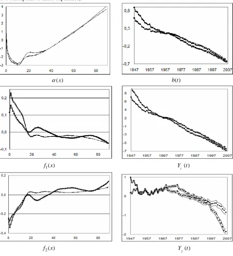
, and the percentage variance explained by the j-component is 2 2

[image:9.595.71.550.269.794.2]

Figure 2, displays the sparse components based on the common age-period (sparse) association model structure (3), for both sexes, from the pooled experience of the West-cluster 19 countries and time period 1947-2006. The optimum number of GLM parameters, by maximizing the Bayesian (or Schwarz) Information Criterion, for both sexes, is k=23. Concerning the graduation process (model structure (1)), the standardized deviance residuals (SDR) plotted against age, time and cohort effects, shows that the overall patterns of the total SDR indicate an appropriate fit, with R-squared statistics 99,92%. The first two (sparse) interaction terms describe the different dynamics of the two age groups. For the males experience, the first two SPCs account for 97.21% of the total adjusted variance explained and for females 98.61% the total adjusted variance explained (after QR decomposition). For males, the first interaction term accounts for 96.14% of the total adjusted variance and refers mainly to young ages 0-17, and for females it accounts for 98.41% and refers mainly to ages 0-35 (positive

f x

₁

( )

values, Figure 2). For males, the ages 18-35 have higher

α

( )x values than females (Figure 2, graph

α

( )x ), and are grouped on the second SPC. Thus, for males, we separate the young 0-17 ages which belong to the most significant mortality dynamic, as described by the graph (the steeper curve corresponds to females experience), and the remaining ages which are described by the graph (the steeper curve corresponds to males experience).

1

( )

Y t

2

( )

Y t

( )x

α

b t

( )

1

( )

f x

1 ( )

Y t

2

( )

f

x

2 ( )

Figure 2: Dynamics in age-time effects based on the commonage-period (sparse) association model structure (3), with associated CIs, for both sexes.

α

( )x &

b t

( )

graphs, display the independent main age and time effects respectively.

( )

i

f x

&

Y t_i( ) graphs (for i=1,2), display the first two (sparse) interaction terms. The shape of the

f x

_i

( )

age profile indicates which age specific rates respond rapidly and which slowly over which period of time, in response to particular time trends in Y t_i( ).

3. Common Sex Difference mortality dynamics

Figure 3, presents the time profile of the sex difference between the common main time trends plus the sex difference between their overall means,

D

(

μ

+

b t

( ))

, and the sex difference between the life expectancies,

0

( ( ))

D e t

. In both graphs, we observe increasing differences up to 1980s and thereafter a decline (in a more accelerated way for life expectancies, in comparison with the main time trend).

(

( ))

[image:10.595.73.552.261.412.2]

D

μ

+

b t

D e t

( ( ))

0

Figure 3: Sex differences, in main common time trends and in common life expectancies, in time effects.

Sex differentials in mortality are normally attributed to trends in behavioral and social risk factors such as cigarette smoking, heavy drinking, violence and occupational hazards (Preston 1970). Also, many authors have discussed the observed narrowing effect in life expectancies between the sexes. Mesle (2004) has stated that sex differences in life expectancies began to narrow, around the 1980s, in the industrialized countries of Northern Europe, Northern America and Oceania. Glei & Horiuchi (2007) have demonstrated that, more recently, the sex differential has begun to decline in Western Europe and appears to be leveling off among several countries in Southern Europe. Attempts to explain the recent narrowing have focused on causes of death, as well as behavioral and medical factors that would lead to reduced sex ratios in mortality rates. These factors include increased smoking among women while its prevalence has declined among men, and advances in medical treatments for cardiovascular disease that have benefited men more than women (Waldrom, 2005).

In order to model the sex differentials and identify the ages which have contributed to the changes in the mortality gap between the sexes, both during the period when it widens (1947-1980) and during the period when it began to narrow (1980-2006), we construct the sex difference common age-period model structure. Based on the males commonage-period graduated model structure (1), we produce a matrix of GLM parameter estimates, of order n by k, of entries, say , for t=1,2,…n and j=1,2,…,k, and a

matrix of graduated logged central mortality rates, of order n by x, of entries , say

1( )

j t

β ₋ BM ={β_j−₁( )t }

ˆ ( )

_x

m t

log(

M

ˆ

)

=

B

M

⋅

L

′

, where L denotes an orthonormalzero-centered polynomial. Let

β

( )

t

denote the GLM estimated multivariate random variable at time t. From the properties of GLMs, each cross-sectional vector of the estimated parameters is a k-dimensional random variable, which follows asymptotically a multivariate k-dimensional normal distribution with associated covariance matrix, say , for each calendar year t. Constructing in an analogous manner the females common age-period graduated model structure, with the same 19 West-cluster countries, we produce another matrix of GLM parameter estimates, of order n by k, say B . The difference between these two matrices, i.e. the random matrix

t

Σ

F

D F

B =B −_BM_{, defines another cross-sectional k-dimensional random}

equal to the difference between the females and males mean, and covariance matrix equal to the sum of the females and males covariance matrices, for each calendar year t.

Applying PCA to the

B

D matrix, we construct the sex difference common age-period model:

1

ˆ

log(

( ))=

( )

( )

( )

( )

x x

p

D D D D

i i

i

m

t

A

x

g

x Y

t

ε

t

=

+

∑

⋅

+

(4)

where the

log(

ˆ

( ))

is the sex ratio of the logged graduated common central mortality rates, i.e. x

D

m

t

ˆ ( )

)

log

ˆ

( )

x

x

F

M

m

t

m

t

=

ˆ

log(

( )

x

D

m

t

, where denotes the males graduated common central mortality rates, and

denotes the females graduated common central mortality rates. Under model (4), we are able to identify the most important components of the sex differential in mortality, in terms of age and time effects.

ˆ

( )

x

M

m

t

ˆ ( )

x

F

m

t

In Figure 4, panels 4.1.a & 4.1.b, display the first interaction component for the time period 1947-1980, which explains 95% of the total variance. We note the widening effect in time trend ( graph), which is

influenced by all of the ages, and especially the age groups 15-35 and 60-75 ( graph). We also note the curvature, and hence the diminishing rate of divergence, in the time trend. These results are similar to those of Glei & Horiuchi (2007), who have concluded that ages 40 and over were the biggest contributors to this increase, and especially ages 60-79 (based on their analysis of the sex differential effects, for 21 countries separately between the years 1950-54 to 1975-79 and 1975-79 to 2000-04, after pooling the data into 5-year time intervals and 5-year age groups).

1

( )

D

Y

t

)

x

1

(

D

g

Panels 4.2.a, 4.2.b, 4.3.a and 4.3.b display the first two interaction components for the second time period 1980-2006. The first interaction term (panels 4.2.a & 4.2.b), shows the narrowing effect for the age groups 0-20 and 40-75, and the widening effect for ages 75+, and it explains 57% of the total variance. The age group 20-40 refers to the second interaction term (panels 4.3.a & 4.3.b), which shows a widening effect until the 1990s and a narrowing thereafter; it explains the 20% of the total variance. These results are in accordance with the findings of Glei & Horiuchi (2007), where the biggest contributors to reducing the mortality gap were those aged 40-79, and in contrast, the mortality of those aged 80 and older continued to have a widening effect on the gap (for all countries execpt USA).

Panels 4.4.a & 4.4.b display the first interaction component for the whole time period 1947-2006, which explains 88% of the total variance. We note the widening effect in the time trend until the 1980s, and the narrowing effect afterwards, which is influenced by all ages, and especially by the age groups 15-35 and 60-75. This is the overall effect from the two different time periods (1947-1980 & 1980-2006) which describe adequately the dynamics of the sex differential in mortality over the whole time period, since the widening effect before 1980s and the narrowing effect after 1980s refer mostly to the same age groups. Glei & Horiuchi (2007) confirm that the age groups which contributed to widening the gap in the earlier period also contributed to the narrowing in this more recent period (between the years 1950-54 to 1975-79 and 1975-79 to 2000-04 respectively).

4.1.a (1947-1980) 4.1.b (1947-1980)

1 ( )

D

g x

1 ( )

D

Y t

4.2.a (1980-2006) 4.2.b (1980-2006)

1 ( )

D

g x

1 ( )

D

Y t

4.3.a (1980-2006) 4.3.b (1980-2006)

2 ( )

D

g x

2 ( )

D

Y t

4.4.a (1947-2006) 4.4.b (1947-2006)

1 ( )

D

g x

1 ( )

D

[image:13.595.92.508.229.408.2]

Figure 4: Dynamics in age-time effects based on the sexdifferencecommonage-period model structure (4), for different

time periods. Left graphs display the age profiles ( ) in response to particular time trends (with associated

i

D

g x ( )

i

D

Y t

CIs). Graphs 4.1.a & 4.1.b display the first interaction component for the time period 1947-1980, graphs 4.2.a, 4.2.b, 4.3.a & 4.3.b display the first two interaction components for the time period 1980-2006, and graphs 4.4.a & 4.4.b display the first interaction component for the whole time period 1947-2006.

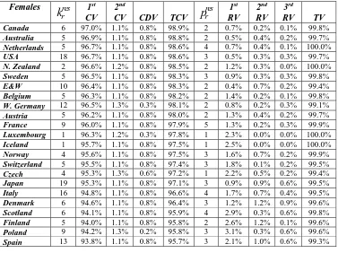
In order to measure how well the common male two-factor model (model structure (2)) and the common male two-factor model plus the common sex difference factor model describes the common female mortality experience, we adopt similar explanation ratios with Li&Lee(2005). Thus, we define the females’ common explanation ratio for the common factor model, say

C

F

R

, and the females’ common explanation ratio for the

augmented common factor model, say AC F

R

:

(

)

1 1 1 1 2 2 1 2

log(

( ))

( )

( )

( )

1

log(

( ))

( )

n a

x

C _{n a}

x

t x

F F

i i

t t x x i

F

t x

F F

t t x x

m

t

A

x

g

x Y t

R

m

t

A

x

= = = = =

⎛

⎞

−

−

⋅

⎜

⎟

⎝

⎠

= −

−

∑ ∑

∑

∑ ∑

=86.8% and

(

)

1 1 1 1 2 2 1 1 1 2

log(

( ))

( )

( )

( )

( )

( )

1

log(

( ))

( )

n a

x

AC _{n a}

x

t x

F F D D

i i

t t x x i

F

t x

F F

t t x x

m

t

A

x

g

x Y t

g

x Y

t

R

m

t

A

x

= = = = =

⎛

⎞

−

−

⋅

−

⋅

⎜

⎟

⎝

⎠

= −

−

∑ ∑

∑

∑ ∑

=96.76%

where

( )

denote the females’ common crude central rates, and x

F

m

t

A

F

( )

x

denotes the females’ main age

profile as constructed by the females’ common model structure.

4. Residual analysis for each country

In this section, we turn to the particularities of the mortality dynamics for each country and consider the residuals after subtracting the two common interaction terms from the pooled mortality model structure (2). This approach follows the suggestions of Lee (2003) and Cairns et al (2008, 2009). Preliminary experiments with the common mortality experience for females (as well as with the common mortality experience for the 2 sexes combined), to model and forecast coherently the country specific experience has shown that the males mortality experience gives more distinct and better results in terms of goodness of fit and forecast performance. Consequently, we base the residual analysis, for both sexes, on the common mortality dynamics for males. Under this approach, we also need the common sex difference mortality dynamics (4) to model the female residuals.

Thus, for the males experience, we consider the residuals for each country, conditional on the main individual age profile, say A x_r( ) and conditional on the two common interaction terms for males:

1,

2

, , , , , , , 1

1 1

log( ( )) log( ( )) log( ) ( ) ( ) ( ) ( ) ( )

res r

j r

k res

x t r x t r x r x t r r i i j

i j

E D R m t R A x g x Y t β t L x

− −

= =

⋅

= ⋅ = + +

∑

⋅ +

∑

This defines the males residual age-period graduated model structure, for each country, where the

2

, ,

1

log( _{x t r}) _r( ) _i( ) _i( )

i

R A x g x Y t

=

+ +

∑

⋅ term is treated as an offset. The main age profiles, , are

estimated separately for each country, since they do not cause mortality divergence. Then, we apply ordinary

( )

r

PC analysis to the associated matrix of these conditional GLM estimates, , leading to the males

residualage-period model structure:

1,

( )

j r

res

_t

β

−

,

( )

t

+

ε

x r,

(

1 1 ) res r k i j t β = = +

∑

∑

, , 2 1 1

ˆ

log(

( ))=

( )

( )

( )

( )

)

res r

i r i r

p

res res

x r r i i

i i

m

t

A x

g

x Y t

g

x Y

t

= =

+

∑

⋅

+

∑

⋅

(5)

Similarly, for the females experience, we consider the residuals conditional on the individual main age profile, , and conditional on the two common interaction terms for males, and conditional on the common sex difference interaction term under model structure (4):

( ) r

A x

1,

2

, , , , 1 1 1

log( ( )) log( ) ( ) ( ) ( ) ( ) ( ( ) ( )

j r

D D res

x t r x t r r i i j

E D R A x g x Y t g x Y t L x

− ⋅ −

= + + ⋅ + ⋅

This defines the females residual age-period graduated model structure, in which the

2

, , 1 1

1

log( x t r) r( ) i( ) i( ) D( ) D( )

i

R A x g x Y t g x Y t

=

+ +

∑

⋅ + ⋅ term is treated as an offset, for each country. Then ,

we apply the eigenvalue decomposition to the associated covariance matrix of these conditional GLM estimates, leading to the femalesresidualage-period model structure, for each country:

, ,

1

( )

i r

res

x Y

⋅

2

, 1

1 1

ˆ

log(

( ))=

( )

( )

( )

( )

( )

( )

( )

res r

i r

p

D D res

x r r i i x r

i i

m

t

A x

g

x Y t

g

x Y

t

g

t

ε

t

= =

+

∑

⋅

+

⋅

+

∑

+

_, (6)

The percentage of the variance explained by each interaction term involved in the residualage-period model structures (5) & (6) (2+

p

_rres interaction terms for males and 3+

p

_rres interaction terms for females) can be

evaluated by QR decomposition on the matrix of all the (S)PCs (2+

p

_rres PCs for males and 3+

p

_rres PCs for females).

The criterion, which will define which residual interaction term will be included in the residual age-period model structures (5) & (6), is based on the following three conditions: a) if the residual variance explained is more than 0,5%, or b) if the confidence level (CL) value is more than 99% (see Hatzopoulos and Haberman (2011), section 2.1) or c) if the residual variance explained is more than 0,1% and the confidence level (CL) value is more than 95%.

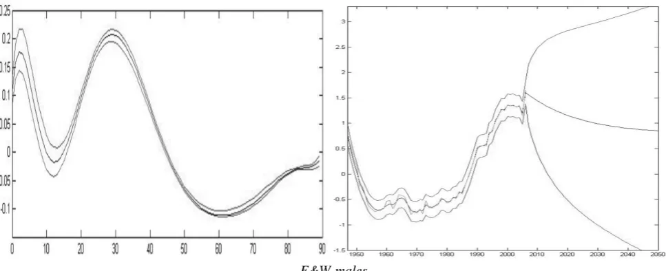
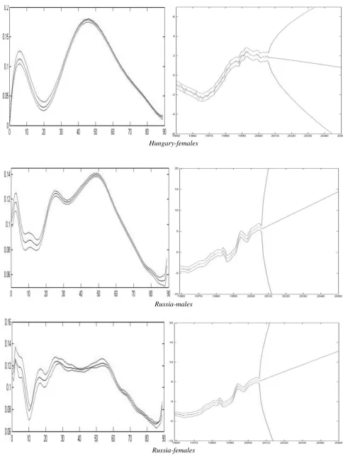
In Tables 2 &3, we give the results obtained according to the residualage-period model structures (5) & (6), for males and females respectively. For each of the 35 countries, we give the first calendar year with available mortality data (after 1947) as provided by the HMD, the number of optimum residual parameters ( values),

and the optimum number of residual interaction terms (

res r

k

res r

p values). Also, we present the common adjusted variances (CV) as explained by the two common interaction terms for males, the common sex difference variance (CDV) for females as explained by the common sex difference interaction term, and the total common variances (TCV) for both sexes. For the female case, the TCV explained is equal to the sum of the adjusted common variance explained plus the adjusted common sex difference variance. The Tables are sorted according to the TCV. Finally, we give the first three adjusted residual variances explained (RV), and the total variance (TV) explained as defined by the sum of the adjusted TCV plus the RVs explained.

Males First year

res r

k

_CV 1st _CV 2nd _TCV

p

_rres _RV 1st _RV 2nd _RV 3rd _TV

Luxembourg 1960 1 97.1% 1.2% 98.3% 1 1.7% 0.0% 0.0% 100.0%

Sweden 1947 4 97.1% 1.1% 98.2% 3 0.8% 0.7% 0.3% 99.9%

Denmark 1947 4 97.1% 1.1% 98.2% 1 0.8% 0.4% 0.5% 99.0%

USA 1947 16 96.7% 1.1% 97.8% 4 0.5% 1.0% 0.2% 99.8%

Norway 1947 4 96.4% 1.1% 97.5% 3 1.0% 1.2% 0.2% 99.8%

N. Zealand 1948 4 96.3% 1.2% 97.5% 2 1.0% 1.1% 0.3% 99.6%

Netherlands 1947 7 96.1% 1.1% 97.2% 3 1.2% 0.6% 0.8% 99.8%

W. Germany 1956 12 96.1% 1.3% 97.5% 1 1.4% 0.3% 0.3% 98.9%

Switzerland 1947 5 96.0% 1.1% 97.1% 3 1.9% 0.6% 0.3% 99.9%

Iceland 1947 1 96.0% 1.1% 97.0% 1 3.0% 0.0% 0.0% 100.0%

E&W 1947 11 95.8% 1.1% 96.9% 3 2.0% 0.3% 0.2% 99.4%

Canada 1947 7 95.6% 1.1% 96.6% 2 2.5% 0.4% 0.3% 99.5%

Belgium 1947 7 95.5% 1.1% 96.5% 3 0.5% 2.1% 0.7% 99.8%

France 1947 15 95.3% 1.1% 96.4% 4 0.9% 1.9% 0.2% 99.5%

Austria 1947 9 95.3% 1.1% 96.3% 3 1.2% 1.1% 0.6% 99.2%

Czech 1950 7 95.2% 1.3% 96.4% 3 1.8% 0.8% 0.4% 99.4%

Australia 1947 9 94.7% 1.1% 95.8% 3 2.5% 0.7% 0.6% 99.4%

Poland 1958 8 94.1% 1.3% 95.4% 2 3.3% 0.4% 0.3% 99.2%

Scotland 1947 5 94.0% 1.1% 95.0% 3 4.3% 0.2% 0.2% 99.8%

Italy 1947 17 93.1% 1.0% 94.1% 4 3.9% 0.5% 0.3% 99.1%

Slovakia 1950 7 92.9% 1.3% 94.2% 2 3.5% 1.2% 0.4% 98.9%

E. Germany 1956 12 92.3% 1.3% 93.6% 5 3.3% 0.3% 1.0% 99.4%

Japan 1947 21 92.0% 1.0% 93.0% 3 4.2% 1.3% 0.7% 99.2%

Ukraine 1959 13 91.2% 1.2% 92.4% 2 5.4% 1.0% 0.5% 98.8%

Ireland 1947 4 90.8% 1.0% 91.8% 3 6.3% 1.3% 0.3% 99.8%

Portugal 1947 14 90.2% 1.0% 91.2% 3 5.4% 1.5% 0.7% 98.8%

Finland 1947 7 90.0% 1.0% 91.0% 2 6.8% 1.2% 0.5% 99.1%

Lithuania 1959 7 89.2% 1.2% 90.3% 4 5.5% 2.1% 1.1% 99.6%

Belarus 1959 10 88.9% 1.2% 90.1% 3 5.2% 3.2% 0.6% 99.0%

Estonia 1959 5 88.2% 1.2% 89.4% 3 8.0% 0.9% 1.2% 99.6%

Latvia 1959 7 87.2% 1.2% 88.4% 3 6.9% 3.2% 0.6% 99.1%

Hungary 1950 9 86.9% 1.2% 88.0% 3 9.1% 1.1% 0.4% 98.7%

Russia 1959 23 86.1% 1.2% 87.2% 3 9.7% 1.7% 0.5% 99.2%

Bulgaria 1947 12 83.8% 0.9% 84.8% 3 13.0% 0.6% 0.8% 99.1%

[image:15.595.124.501.512.794.2]

Spain 1947 15 83.6% 0.9% 84.5% 3 13.1% 0.5% 1.1% 99.2%

Table 2: Males starting calendar year, number of optimum GLM residual parameters, common and total common variance explained, optimum number of residual interaction terms, residual variance explained for each residual interaction term and total variance explained, for each country.

Females res r

k

_CV 1st _CV 2nd _{CDV TCV}

p

_rres _RV 1st _RV 2nd _RV 3rd _TV

Canada 6 97.0% 1.1% 0.8% 98.9% 2 0.7% 0.2% 0.1% 99.8%

Australia 5 96.9% 1.1% 0.8% 98.8% 2 0.5% 0.4% 0.2% 99.7%

Netherlands 5 96.7% 1.1% 0.8% 98.6% 4 0.7% 0.4% 0.1% 100.0%

USA 18 96.7% 1.1% 0.8% 98.6% 3 0.5% 0.3% 0.3% 99.7%

N. Zealand 2 96.6% 1.2% 0.8% 98.5% 2 1.2% 0.3% 0.0% 100.0%

Sweden 5 96.5% 1.1% 0.8% 98.3% 3 0.9% 0.3% 0.3% 99.8%

E&W 10 96.4% 1.1% 0.8% 98.3% 2 0.4% 0.7% 0.2% 99.4%

Belgium 5 96.3% 1.1% 0.8% 98.2% 2 1.4% 0.2% 0.1% 99.8%

W. Germany 12 96.5% 1.3% 0.3% 98.1% 2 0.8% 0.2% 0.3% 99.1%

Austria 5 96.2% 1.1% 0.8% 98.0% 2 1.3% 0.4% 0.2% 99.7%

France 9 96.0% 1.1% 0.8% 97.9% 5 1.3% 0.2% 0.3% 99.9%

Luxembourg 1 96.3% 1.2% 0.3% 97.8% 1 2.3% 0.0% 0.0% 100.0%

Iceland 1 95.7% 1.1% 0.8% 97.5% 1 2.5% 0.0% 0.0% 100.0%

Norway 4 95.6% 1.1% 0.8% 97.5% 3 1.6% 0.7% 0.2% 99.9%

Switzerland 5 95.5% 1.1% 0.8% 97.4% 3 1.8% 0.1% 0.2% 99.5%

Czech 4 95.3% 1.3% 0.6% 97.2% 1 2.2% 0.5% 0.2% 99.4%

Japan 19 95.3% 1.1% 0.8% 97.1% 3 0.9% 0.9% 0.6% 99.5%

Italy 16 94.8% 1.1% 0.8% 96.6% 4 1.7% 0.7% 0.4% 99.5%

Denmark 6 94.6% 1.1% 0.8% 96.4% 3 1.2% 1.2% 0.9% 99.6%

Scotland 6 94.1% 1.1% 0.8% 95.9% 4 2.9% 0.3% 0.6% 99.8%

Finland 5 94.0% 1.1% 0.8% 95.8% 2 2.6% 1.2% 0.1% 99.6%

Poland 9 94.2% 1.3% 0.2% 95.8% 3 3.1% 0.3% 0.6% 99.6%

E. Germany 6 94.0% 1.3% 0.3% 95.6% 2 3.2% 0.7% 0.2% 99.5%

Portugal 13 93.7% 1.1% 0.8% 95.5% 3 1.4% 1.7% 0.4% 99.0%

Slovakia 4 93.5% 1.3% 0.6% 95.3% 3 3.7% 0.6% 0.3% 99.9%

Ireland 4 93.4% 1.0% 0.8% 95.2% 4 3.6% 0.5% 0.6% 100.0%

Ukraine 14 93.3% 1.3% 0.2% 94.8% 2 3.1% 0.5% 0.8% 98.3%

Belarus 5 93.2% 1.2% 0.2% 94.7% 2 3.7% 1.0% 0.4% 99.4%

Hungary 8 92.3% 1.2% 0.6% 94.2% 3 4.2% 0.5% 0.6% 99.5%

Lithuania 5 91.0% 1.2% 0.2% 92.5% 3 5.5% 1.0% 0.7% 99.6%

Bulgaria 10 90.2% 1.0% 0.7% 92.0% 3 5.8% 0.6% 0.9% 99.2%

Russia 25 90.5% 1.2% 0.2% 92.0% 3 5.3% 1.2% 0.7% 99.1%

Latvia 5 90.3% 1.2% 0.2% 91.8% 3 6.1% 1.2% 0.6% 99.6%

[image:16.595.123.500.62.193.2]

Estonia 2 88.8% 1.2% 0.2% 90.2% 2 9.4% 0.4% 0.0% 100.0%

Table 3: Females starting calendar year, number of optimum GLM residual parameters, common and total common variance explained, optimum number of residual interaction terms, residual variance explained for each residual interaction term and total variance explained, for each country.

5. Coherent Forecasts

As described in section 4, for the construction of the residualage-period model structures (5) & (6), we treat the

term as an offset in the GLM structure. According to the discussion in section 2, the offset

term can be rewritten: , where

2

1

( )

( )

i i

i

g

x Y t

=

⋅

∑

1

( )

( )

( )

b t

′ +

f x

⋅

Y t

Y t

( )

=

Y t

₁

( )

− ⋅

a Y t

₂

( )

and b t′ = ⋅ ⋅( ) l a Y t

[

₁( )+Y t₂( )

]

, for . As a result, the offset term consists of two different mortality dynamics: the main time trend, which encapsulates the overall mortality dynamics for both age ranges (the first age range refers to young ages 0-17, and the second age range refers to adult ages 18+), and a second time trend, which describes the relative divergent trend from the main time trend between the two age groups.

0 e1,2

= ⋅

l L

Figure 5 displays the offset component according to the males common age-period (sparse) association model structure (3), from the common experience of the West-cluster 19 countries, for time period 1947-2006. The main time trend (Figure 5, panel 5.1.b) exhibits a linear trend since the 1970s. The term (Figure 5, panel 5.2.b) describes the relative divergent trend from the main time trend between mortality rates for the young and for adults. With reference to the

( )

Y t

1

( )

f x

( )

Y t

age profile (positive values for the young ages and negative values for the adult ages, Figure 2), the trend indicates a faster mortality improvement for the young (and slower mortality improvement for the adults) than the main time trend. Meanwhile, the concave shape of the trend reveals that the faster mortality improvement for the young (than the main time trend) decreases with time and at the same time the relative slower mortality improvement for the adults increases with time.

( )

Y t

Similarly to the approach of Hatzopoulos and Haberman (2009, 2011), we utilize dynamic linear regression (DLR) model structures. The DLR time series models are simply regression models in which the explanatory variables are functions of time and the parameters are time-varying. State space models employ the Kalman filter technique through which smoothed estimates of the stochastic parameters and predicted future values (Harvey, 1991) can be derived. The computations have been implemented in Matlab using the Captain Toolbox (Taylor, 2007).

t

dynamics. The represents the overall rate of mortality improvements, which has a (smoothed) rate of mortality improvements of 0.0212 at calendar year 2006 and an extrapolated rate of mortality improvements of 0.0222 at calendar year 2050. Experiments with the males common central mortality trends, as described in section 2, show decreasing rate of mortality improvements for the young ages and accelerating rates for the old ages. The observed main time trend, which summarizes the mortality movements from all the ages, displays an almost linear trend since the 1970s, and an extrapolation of this feature seems to be a plausible choice. Panels 5.1.a & 5.1.b describe the dynamics and the forecasts of the main time trend. The ACF and the PACF indicate an acceptable residual structure and the Lillilifors test has a 3.9% p-value.

1,t

b

( )

Y t

Next, we model the time trend, which describes the relative deviations from the main time trend. We use a DLR structure:

( )

Y t

2 b2,t t e2,

α

= + ⋅ + , with the slope being a stochastic time variable parameter that follows a

first order autoregressive (AR(1)) process: b_2,t =

ϕ

₂⋅b_{2, 1t−} +

ζ

_{2, 1t−} (smoothed rates are shown at graph 5.2.a, with associated estimated value

2,

ˆ

t

b

2

ˆ

ϕ

=0.99 (0.06)). The innovations

e

_2,t and

ζ

_2,t are assumed to be white noises random variables, with associated standard deviations 0.16 and 0.0035 respectively. The coefficient of determination is 99.7%. Under this structure, the tends to a constant level, which causes ultimately identical rate of mortality improvements, for each age group. The ACF and the PACF indicate an acceptable residual structure, the Lillilifors test has a 50% p-value, and the Jarque-Bera test has a 93% p-value.

( )

Y t

The above DLR model structures cause particular trends to the associated SPCs (

&

)

, as displayed in panel 5.3.a. For the 1st SPC, which describes mostly the mortality experience of the young, we forecast (slightly) decreasing rates of mortality decline, with the rate of improvement equal to 0.22 at calendar year 2006 and a forecast rate of improvement of 0.16 at calendar year 2050. Lee (2005) and Wilmoth (1998), Oeppen and Vaupel (2002) and White (2002), discuss the processes of catch-up and convergence. They argue that some countries converge toward the leader (e.g. Japan), and in preparing mortality forecasts for a given country, the extrapolated trend for the leader country should form the basis for a long-run scenario. As defined by Wilmoth (1998), the leader country at any given point in history is the country whose overall level of mortality equals the minimum achieved at that time by any national population. If we represent the overall level of mortality with the overall means (Table 1,

1

( )

Y t

Y t

₂

( )

r

μ

-values), then the most important leader countries, for the time period 1960-2006, are Sweden, Netherlands, Japan and Norway, for both sexes. The (sex combined) common mortality trends, constructed from these 4 leader countries, show a decreasing rate of mortality improvements for the very young ages (we obtain the same results from the construction of the common mortality trends, utilizing 19 West-cluster countries). Therefore, if we base the future mortality dynamics on the decreasing rate of mortality progress from the leader countries, then we are in accordance with the forecast 1st SPC trend. For the 2nd SPC, the above modelling produces almost steady rates of mortality improvements, with the rate of mortality improvement equal to 0.135 at calendar year 2006 and a forecast rate of mortality improvement of 0.137 at calendar year 2050. This leads to a forecast that adult mortality rates follow an almost linear trend, which follows the dynamics since 1990s (panel 5.3.a). White (2002) has noted that the predominant types of mortality reduction has shifted from curing infectious diseases, that heavily affect the young, to degenerative diseases that largely affect the elderly, and noted that this transition was neither instantaneous nor absolute. He has concluded that the major targets for mortality decline in the near future will probably be the same as over the past four decades. Experiments with the sex combined, common mortality trends, constructed from the 4 leader countries, show a steady rate of mortality improvement for the adult ages and an increasing rate of mortality improvements for the old ages. This remark is in accordance with the forecast 2nd SPC (panel 5.3.a), which describes the dynamics of adult mortality.

t

For the females experience, according to the females residual age-period model structure (5), we model the common sex difference PC, with a DLR model:

1 ( )

D D D t

Y t =α +b ⋅ +t e , with the slope being a stochastic time

variable parameter that follows a first order autoregressive process. In panel 5.4.a, we show the smoothed

ˆ

t

D

b

estimated values, from the common sex difference PC, which follow a first order autoregressive process with

ˆ

ϕ

=

1

ˆ (

D

Y

0.9819 (0.029). Under this DLR model structure, we achieve coherent forecasts for both sexes, since the

trend reaches a constant value (panel 5.4.b). The ACF and the PACF indicate an acceptable residual structure: Lillilifors test has a 50% p-value, and the Jarque-Bera test has a 93% p-value.

)

t

5.1.a DLR forecast rates,

b

ˆ

_1,t, for b t′( ) 5.1.b forecast common main time, b tˆ ( )′

5.2.a DLR forecast rates,

b

ˆ

_2,t, for Y t( ) 5.2.b forecast relative deviations,

Y t

ˆ( )