A metamodeling framework for extending the application domain of process-based ecological models

of process-based ecological models

1

Department of Plant Pathology, Kansas State University, Manhattan, Kansas 66506-5502 USA

2

International Potato Center, Apartado 1558, Lima 12, Peru

3_{Department of Environmental Science and Policy, University of California, Davis, California 95616 USA}

Citation:Sparks, A. H., G. A. Forbes, R. J. Hijmans, and K. A. Garrett. 2011. A metamodeling framework for extending the application domain of process-based ecological models. Ecosphere 2(8):art90. doi: 10.1890/ES11-00128.1

Abstract. Process-based ecological models used to assess organisms’ responses to environmental conditions often need input data at a high temporal resolution, e.g., hourly or daily weather data. Such input data may not be available at a high spatial resolution for large areas, limiting opportunities to use such models. Here we present a metamodeling framework to develop reduced form ecological models that use lower resolution input data than the original process models. We used generalized additive models to create metamodels for an existing model that uses hourly data to predict risk of potato late blight, caused by the plant pathogenPhytophthora infestans. The metamodels used daily or monthly weather data, and their predictions maintained the key features of the original model. This approach can be applied to other complex models, allowing them to be used more widely.

Key words: climate change scenario analysis; data aggregation; ecoinformatics; ecological scaling; metamodels;

Phytophthora infestans; plant disease; process-based models;Solanum tuberosum.

Received 4 May 2011; accepted 20 May 2011; final version received 27 July 2011; published 18 August 2011. Corresponding Editor: S. Collinge.

Copyright:Ó2011 Sparks et al. This is an open-access article distributed under the terms of the Creative Commons Attribution License, which permits restricted use, distribution, and reproduction in any medium, provided the original author and sources are credited.

4

Present address: International Rice Research Institute, DAPO Box 7777, Metro Manila, Philippines.

 E-mail:[email protected]

I

There is growing interest in process-based modeling approaches to study the distribution of species (Chuine and Beaubien 2001, Kearney and Porter 2004, Morin et al. 2007, Jackson et al. 2009, Monahan 2009, Buckley et al. 2010), but data requirements for both model development and application have limited the types of questions that can be addressed with these approaches. There is also increasing interest in using such models for strategic assessments of the value of new management practices (Hijmans et al. 2003) and responses to climate change (Rosenzweig and Parry 1994, Hijmans 2003, Audsley et al. 2008, Luedeling et al. 2009).

However, modeling the distribution of species over larger areas is dominated by correlative approaches (Guisan and Thuiller 2005, Elith and Leathwick 2009). This is in part because of the absence of process-based models for many species, but also because the large extent - high resolution data sets needed to apply such models often are not available.

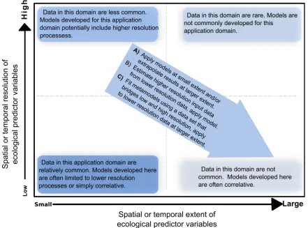
1994). Even for plants and animals with long generation times, many ecophysiological pro-cesses occur at short time scales (e.g., an extreme frost event; Hijmans et al. 2003). Process-based models have been used, for example, to study the growth and development of crops (De Wit and Brouwer 1971) and crop disease (Van der Plank 1963), to simulate greenhouse gas emissions from soil (Li et al. 1992, Giltrap et al. 2010), and to predict the spatial distribution of species (Kear-ney and Porter 2004). The need for high temporal resolution input data can make it very cumber-some, or impossible, to use such models over large spatial extents (Fig. 1; Morin and Lecho-wicz 2008, Thuiller et al. 2008, Randin et al. 2009). Here we develop an approach for adapting models that were developed using input data with high temporal resolution, so that they can be used with lower resolution input data.

There have been two main approaches for applying models across large areas for which high temporal resolution data are not available: (1) The model is applied for locations where sufficient data are available (e.g., a limited number of weather stations supplying daily weather data) with predictions interpolated between these locations/times (De Wolf et al. 2002, Wu et al. 2006). (2) Higher resolution input data are generated from lower resolution input data; for example, small time-step weather such as rainfall patterns can be generated from larger time-step data through stochastic weather gen-erators (e.g., Wilks and Wilby 1999, Hijmans et al. 2000). Both of these approaches have draw-backs. Interpolation between stations that are far apart may not adequately capture the non-linear effect of weather on the model organism. Stochastic simulation of weather data is compli-cated and computationally intensive, and the response model needs to be run many (e.g., 100) times to obtain an average response. Here we develop an alternative approach, (3) the use of metamodels, adapting a model so that it can be used with lower resolution input data. The term metamodel can refer to a simplification of the original model that retains its salient features, or to a single model created by combining the results of multiple models. In this paper we present a metamodeling framework to extend the application domain of a model, so that the metamodel can be applied to lower temporal

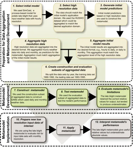
resolution weather or climate data. Metamodels have been developed in bio-economics (Laksh-minarayan et al. 1996, Breukers et al. 2007, Kristensen et al. 2008), and in manufacturing industries to improve design optimization (Wang and Shan 2007). In ecology they have been used to organize and synthesize models (Slobodkin 1958), to facilitate the study of endangered species risk assessments (Nyhus et al. 2007), and to assess impacts of socio-economic and climate change on wetlands (Harrison et al. 2008). Lastly, in ground water management metamodels have been used as a way to reduce model complexity while keeping those processes and parameters for which the simulation output is sensitive, or for which input data are available (Tiktak et al. 2006). Many metamodels have been constructed to consolidate different models into a single model, but to our knowledge they have not been used in ecology to extend the applica-tion domain of the original model as we do here. Our framework for metamodel development consists of the following steps (Fig. 2). (1) A well-validated initial process-based model is available that would be desirable to use, but its application is limited to high resolution input data. (2) A large, high resolution, input data set is selected to match the requirements of the initial model, and to be representative of the types of conditions in which we would like to apply the resulting metamodel. (3) The initial model is applied to generate predictions from the input data set. (4) A second set of input data is generated by averaging to the level of aggregation at which such data are more generally available. (5) If predictions from the initial model are higher resolution than output from the new metamodel will be, a second set of predictions is generated by averaging the high resolution predictions to the desired level of aggregation. (6) The aggre-gated data of step 4 (and step 5 as needed) are divided into model construction and evaluation sets. (7) The metamodel is constructed to describe the relationship between the aggregated input data and aggregated predictions from the initial model. (8) The metamodel performance is evaluated for the evaluation data set. (9) The metamodel is evaluated in terms of potential limitations, in general and in comparison to the initial process-based model.

Phytophthora infestans (Mont.) De Bary., the proximate cause of the Irish potato famine) as a model system for application of this framework because it is well-studied, with well-validated high resolution models available, and its ecology illustrates the type of sensitivity to high resolu-tion variaresolu-tion in weather that is common to many microbes and arthropods. Late blight forecasting models recognize the importance of temperature and moisture in disease development, and have evolved over time using combinations of these variables for forecasting. The earliest of these models for predicting late blight risk were the

‘‘Dutch Rules’’ postulated by Van Everdingen (1926, and discussed in Beaumont (1947)). Fry et al. (1983) developed SimCast, a predictive late

consecutive hours over 90%RH, the temperature

(T) during those intervals, and genotype-specific

host resistance to disease. SimCast is typical of

aspect of the infection process: periods of moisture must occur, at disease-conducive tem-peratures that last long enough to support foliar infection. Hijmans et al. (2000) used these types of models at a global scale to estimate the number of pesticide applications necessary to manage late blight, using monthly climate data and a weather generator (approach 2 described above) for dealing with low resolution weather data. Because SimCast has become well-estab-lished as a successful tool for late blight management and research (Skelsey et al. 2009) in many areas of the world, we used it for development of potato late blight metamodels.

Our overall goal in this study was to provide a framework for constructing metamodels that can readily be applied to scaling ecological models, thereby extending their application domain from high resolution input data to low resolution input data, and thus supporting their application across large extents. We developed a metamodel of the SimCast potato late blight risk model. Our primary objective was to develop disease risk models that use monthly or daily weather data as input, and compare the predictions made with these models to predictions made with the initial model that uses hourly weather data. This type of application domain extension has many potential applications for scenario analysis for potato late blight, specifically, and as an example of the potential for scaling other models. A secondary objective was to compare the perfor-mance of models constructed using targeted weather data from regions where the host of the disease occurs, with the performance of models constructed using a data set that repre-sents a broader range of climates. As indicated under step 2 of the framework described above, the data set used for metamodel construction should be representative of intended application scenarios for the model, but it is an open question whether the targeted or broad approach is best.

M

Our first objective was to develop disease risk metamodels for use with temporally aggregated weather data and compare the performance of these models with the original model that uses high resolution input data. As step (1) in the metamodeling framework (Fig. 2), we had

identified SimCast as a model that has been well-validated in a number of environments, but requires hourly temperature and relative humid-ity data as input. (2) We needed a data set with wide geographic coverage, hourly reporting, and extensive data quality control. The National Climatic Data Center Hourly United States Weather Observations (HUSWO) 1990–1995 meet these criteria (US-EPA and NOAA 1997), containing hourly weather observations from 262 National Weather Service stations nationwide. Data from the 247 stations reporting hourly temperature, relative humidity, and precipitation were included in the analysis. Weather data from the US represent all five of the main groups of the Ko¨ppen-Geiger climate classification system, and 22 of 31 climate classes (Kottek et al. 2006, Rubel and Kottek 2010); classes not represented are unlikely to support potato production. HUSWO data were split into two subsets for model construction (1990–1992) and model evaluation (1993–1995). (3) Blight units for each day at each location in the HUSWO data set were predicted for susceptible and resistant genotypes using SimCast as presented in Gru¨nwald et al. (2002). These ‘true’ blight units based on predictions from hourly input would then be used as the standard for analysis of the metamodels. (4) We were interested in comparing metamodels for both daily and monthly resolution. The HUSWO data were averaged (within each location) to provide day-resolution and month-resolution aggregated input data. So, for example, each HUSWO location-year supplied 12 months of month-resolution data and 365 or 366 days of day-resolution data. It could be argued that consecutive days and adjacent locations are not statistically independent because of autocorrela-tion in weather patterns, but the large size of this data set makes lack of strict independence unimportant. (5) SimCast takes hour-resolution input data and produces day-resolution predic-tions, so ‘true’day-resolution blight units were generated without the need for any aggregation step. To produce ‘true’ month-resolution blight units, the‘true’day-resolution blight units were aggregated.

directly compare the performance of simpler and more complex models. The form of SimCast (Gru¨nwald et al. 2002) suggested a simple linear model would not be sufficient. We developed and tested GAMs to model the relationship between aggregated weather data and aggregat-ed ‘true’ blight units (Table 1). The first GAM metamodel had the form of a simple linear model for the sake of comparison, with blight units (BUi) as the response variable, and temperature

(Ti) and relative humidity (RHi) as predictor

variables, where i indicates the ith location-day (or location-month) in the HUSWO data set for the model construction interval 1990–1992. The second general form of GAM metamodel again had Ti and RHi as predictor variables, but used

the penalized regression spline smoothed func-tion of their interacfunc-tion, withkas the dimension of the basis used to represent the smoothing term (Wood 2006). Daily and monthly resolutions were evaluated for both susceptible and resistant potato genotypes. The metamodels were con-structed in the R environment (R Development Core Team 2010) using the contributed package MGCV (Wood 2008). In the rare cases when blight unit values were predicted to be less than zero, they were set equal to zero. Models were evaluated based on their Generalized Cross Validation (GCV) scores, AIC (Akaike Informa-tion Criterion (Akaike 1974)), and R-squared values.

(8) The metamodel was then evaluated with the evaluation data subset from the years 1993– 1995. We compared Pearson’s correlation coeffi-cients for the SimCast predicted values and the

metamodel predicted values (Table 2). The daily metamodel (mmDaily) predictions could be

com-pared directly, but to compare with the monthly metamodel (mmMonthly) outputs, SimCast blight

unit predictions were averaged, creating an average of daily blight unit accumulation per month.

The secondary objective was to compare the performance of models constructed using weath-er data sets specific to host regions, areas whweath-ere potato is grown within the US, with models constructed using a data set that represents a broader range of climates. Data from Hijmans (2001) were used to determine which of the HUSWO station locations were within potato growing regions in the US. Weather stations in the potato growing areas or within a distance of 10 kilometers were selected and a subset of weather data from these stations was created for use in metamodel construction as detailed in objective one.

R

Metamodel construction and fit

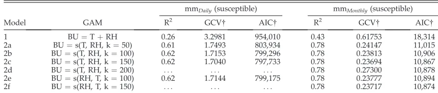
The models that considered an interaction of temperature and relative humidity yielded lower AIC and GCV scores than the model that did not (Table 1), indicating better fit. For mmDaily a k

value of 100 was selected (Fig. 3). Askincreased to 150, the time to run the model increased and the gains in fit were small (Model 2d; Table 1). For mmMonthlyk¼150 was selected (Fig. 3). When

k ¼ 200, mmMonthly begins to decrease in

performance with higher GCV and AIC values (Model 2f; Table 1). The resulting GAM surfaces

Table 1. Performance of metamodels. In the generalized additive model (GAM) equations, BU is blight units, T is temperature, RH is relative humidity, s indicates that the interaction of the variables is smoothed, and k is the dimension of the basis used to represent the smooth term. P-values are all,0.01 and,0.001 for mmDailyand mmMonthly, respectively.

Model GAM

mmDaily(susceptible) mmMonthly(susceptible)

R2 _{GCV  AIC  R}2 _{GCV  AIC} 

1 BU¼TþRH 0.26 3.2981 954,010 0.43 0.61753 18,314

2a BU¼s(T, RH, k¼50) 0.61 1.7493 803,934 0.78 0.24147 11,015

2b BU¼s(T, RH, k¼100) 0.62 1.7153 799,296 0.78 0.23813 10,906

2c BU¼s(T, RH, k¼150) 0.62 1.7040 797,733 0.78 0.23694 10,867

2d BU¼s(T, RH, k¼200) . . . 0.78 0.27300 10,878

2e BU¼s(RH, T, k¼100) 0.62 1.7144 799,175 0.78 0.23777 10,894

2f BU¼s(RH, T, k¼150) . . . 0.78 0.23717 10,874

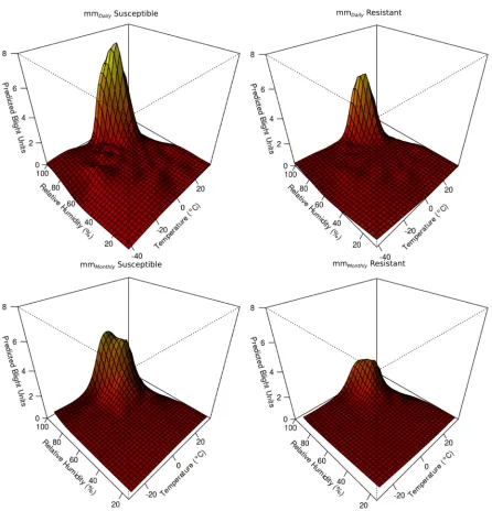
indicate the type of interaction between temper-ature and relative humidity for predicting the accumulated blight units (Fig. 3) that might reasonably be expected based on the structure of SimCast (Gru¨nwald et al. 2002). Once the metamodel forms were selected, metamodels for resistant genotypes were also constructed using these forms of GAM for mmDaily resistant and

mmMonthlyresistant (Fig. 3).

SimCast versus mm

and mm

metamodels

Metamodel predictions for both model con-struction and model evaluation data sets were similar to the results obtained with the original SimCast model (Fig. 4). mmDaily had Pearson’s

correlation scores of 0.85, 0.84 for construction and evaluation data sets, respectively. The correlation scores for mmMonthly for construction

and evaluation data sets were both 0.89. The number of accumulated blight units per day was underpredicted by both mmDaily and mmMonthly,

but predictions by the latter were closer to the SimCast predicted averages (Table 2). While there were large differences between the model predictions, the metamodels successfully cap-tured the main trends and rankings predicted by SimCast (Fig. 4).

The structure of SimCast (Gru¨nwald et al. 2002) causes the accumulation of six or seven blight units per day to occur less frequently than other blight unit values. The weather conditions required for these values to register are ideal for late blight development; seven blight units requires 13–24 hours of a temperature at 13– 228C with the relative humidity above 90%. This is not a problem for SimCast’s typical applica-tions, but it does mean that there were relatively

fewer observations for fitting the GAM at six and seven blight units, and the model exhibits slightly different behavior for these values (Fig. 4) for a susceptible genotype.

Comparison when using potato growing areas only

to construct GAM

The metamodels showed little difference in performance when created from the whole US weather data set or data sets constructed from potato growing regions of the US. Both meta-models under predicted blight units when compared to blight units predicted by SimCast, although again, the mmMonthly metamodel

pre-dictions were closer. However, both metamodels maintain a high correlation with SimCast blight units (Table 2). Similarly the application of a model created using the whole US data set when applied to just potato growing regions showed little difference from a model created using the whole US data set and applied to the whole US. Goodness-of-fit values were similar for all com-binations tested (Table 2).

D

We used a metamodel framework to create a new model based on an ecological model that needs high temporal resolution input data, so that it can be applied with low temporal resolution input data that may be available at a relatively high spatial resolution over large extents. In the discussion we focus on the different steps of the metamodel framework (Fig. 2) in relation to the potato late blight model and more generally for other ecological models.

(1) There is potential for metamodel construc-tion for a wide range of mechanistic models. Table 2. Goodness of fit and Pearson’s Correlation scores of mmDailyand mmMonthly metamodels when fit to SimCast-predicted blight units for construction (Con.) and evaluation (Evn.) datasets for complete US weather data and construction datasets based only on potato producing areas of the US. The SimCast model uses hourly weather data to predict blight units based on hourly weather data. The mmDaily and mmMonthly metamodels predict blight units based on daily and monthly time-step weather data, respectively.

Region

mmDaily mmMonthly

R2 _{p Con. Evn. R}2 _{p Con. Evn.}

All US (Susceptible) 0.62 ,0.001 0.85 0.84 0.78 ,0.001 0.89 0.89

US potato regions (Susceptible) 0.62 ,0.001 0.76 0.74 0.83 ,0.001 0.91 0.91

All US (Resistant) 0.65 ,0.001 0.81 0.81 0.76 ,0.001 0.88 0.88

Models for many plant diseases are similar to the late blight model in that they use weather thresholds which, when crossed for defined brief time periods, trigger a predicted increase in disease risk in the model (e.g., Cu and Phipps 1993, Momol and Aldwinckle 2000). For other diseases, inputs related to phenology of the host

models that are based on limiting factors for survival, such as components of PHENOFIT (Chuine and Beaubien 2001) and CLIMEX (Sutherst and Maywald 1985), depending on their response to extreme input values.

The sensitivity of the initial model to extreme input values, in combination with the tendency or lack thereof for extreme input values to

includes a threshold RH value for infection to occur, it is sensitive to extreme values, and to the interaction between RH and temperature. How-ever, enough of the high resolution features were maintained in the average values that the ordering, though not the absolute values, of the initial model output were maintained in the metamodel output.

(2) The high resolution data used for meta-model construction need to have several charac-teristics. The data need to match the initial model’s application domain, in the case of SimCast having weather data available with hourly resolution. The data need to be such that they can be modified to match new desired application domains. This can generally be accomplished through data aggregation, in the case of SimCast by aggregating the hourly data to produce daily and monthly means. The data need to be extensive enough to provide good coverage of existing variation in weather pat-terns. In our case, the fit of potato late blight metamodels developed using a broad data set (all the US weather data) or a targeted data set (only those from potato-growing regions) were essentially the same. We chose to use the models constructed using the whole US weather data set. This approach represented a broader range of climates and was thus potentially more suitable for global predictions. In fact, the HUSWO weather data set may be equally useful for many ecological models that need to be adapted from requiring high resolution weather data input to lower resolution input data. The HUSWO data are extensive enough that, in our system, the fit of models for the evaluation subset of the data was essentially the same as for the construction subset. Finding large higher resolution input data sets for other types of predictor variables may be more challenging. In such cases, simulated input data (e.g., from a stochastic weather generator) could perhaps be used for construction of the metamodel.

(3–5) The degree to which data can be aggregated for model input is dependent on the system being modeled. Because potato grows over a period of months and is grown in many areas of the world at different times of the year, and late blight is polycyclic, it is most practical to aggregate data to the monthly level. The appro-priate level of aggregation remains to be

deter-mined for other systems such as plant diseases with a narrow window of infection, including fireblight, where blossom infection occurs within a two to four day window (Thomson 2000) or Fusarium head blight of wheat and barley, where infection only occurs during anthesis (De Wolf et al. 2002). If the key input values for determining the response are in a tail of the distribution of input values, the effect may not be preserved. In our case, mmDaily and mmMonthly maintain

rela-tive relationships. If a true one-to-one relation-ship between the original model and metamodel is necessary, the key input values would need to be conserved through averaging.

(6–7) For construction of the metamodel, we used GAMs to model the relationship between the aggregated initial model output and the aggregated weather data input. GAMs have the benefit of flexibility for fitting potentially irreg-ular surfaces resulting from complex ecological interactions. Because they capture irregular sur-faces well, their use puts additional emphasis on the requirement that the data set used for metamodel construction be large and represen-tative. Other smoothing functions could also be used, and for simpler models low order polyno-mial models may be sufficient. In our case, simpler versions of the GAM model that did not include the interaction between temperature and RH performed poorly. In some cases, a priori model structures may be used. It can be argued that use of smoothing functions results in a metamodel that is once more, in some sense

‘correlative’. However, the metamodel incorpo-rates much of the complex information embed-ded in the structure of the process-based initial model, which will tend to provide advantages over approaches such as climate matching.

important. It would be ideal to have ‘response’

data corresponding to the high resolution input

‘predictor’data used to construct the metamodel across a large spatial or temporal extent, but that scenario will be rare. At least it may be possible to evaluate the performance of the new meta-model for a limited number of observations.

The metamodel will tend to have all the limitations of the initial model, other than the requirement for higher resolution input data, and may have additional limitations, as well (though it may be less sensitive to outliers). In the case of potato late blight, SimCast provides an estimate of daily disease risk, but does not incorporate factors such as the potential‘compound interest’

buildup of pathogen populations through the season (e.g., Garrett et al. 2009, 2011). There is also the potential for pathogen populations to evolve such that temperature optima shift, or so that resistance to the pathogen population is less effective. Thus, the metamodel shares these limitations. The metamodel construction frame-work performed well for scaling the model of disease risk based on hourly weather input to metamodels using daily or monthly average weather inputs. Predictions from both the daily and monthly resolution metamodels were strongly and positively correlated with predic-tions from the original hourly resolution SimCast model (Table 2). The salient features of SimCast were maintained in the metamodels, even though the relationship was not one to one. A limitation of this metamodel is that, although it preserves relative changes in disease risk, it does not preserve absolute changes. Interestingly, the fit of mmMonthly when regressed on SimCast

output was slightly better than that of mmDaily.

Reasons for this may include the smoothing effect that averaging has on the SimCast data. Averaging tends to obscure extreme events, but the general relationship is preserved. Apparently monthly averaging maintains the relationship between predictor and response variables better than daily averaging. Maintenance of relative but not absolute features of model predictions may be a common outcome for other model systems, limiting applications to comparative analyses.

In addition to the importance of metamodels such as the late blight metamodel for ecological analysis and planning, the structure of the resulting metamodels is also of inherent interest.

Ecological models, such as those predicting species distributions or disease risk, transform time series of meteorological data into ecological outcomes, in what can be considered summariz-ing or aggregatsummariz-ing data. It is an empirical question whether use of lower temporal resolu-tion weather data will capture the most impor-tant features of a model. De Wit and Van Keulen (1987) suggested that one should‘calculate first, average later’; and Nonhebel (1994) showed that, because of the high variability of the distribution of rainfall in most climates, and the non-linear response of a crop to rainfall, a crop model overestimated potential yield when using month-ly rather than daimonth-ly data. However, these authors did not adjust their models as they aggregated the input data used.

While predictions based on means may not capture all the features resulting from increased variability in the future as a result of climate change (Scherm and van Bruggen 1994), these metamodels are useful tools for decision-making, planning future research and other policy deci-sions. Rather than being a tool for estimating absolute disease risk, our late blight risk evalu-ations are a way of efficiently estimating relative rankings of risk over large areas. Because the late blight metamodels maintain relative relation-ships, despite under predicting blight units, linking these models with a geographic informa-tion system supports creainforma-tion of maps for comparisons between different time-periods un-der climate change scenarios, or comparisons of different geographic areas during the same time period. These types of information for potato late blight can be useful in planning breeding program locations, making determinations re-garding education and extension efforts for areas where disease pressure will increase under future scenarios, or making predictions regarding spe-cies invasions.

the need to estimate shifts in ecological processes such as disease risk more pressing. Because most available climate change data are not at a temporal resolution that is compatible with many currently used process-based models, modifica-tions such as these are particularly useful. Our comparison of metamodels developed from a process-based ecological model indicates that such an approach can successfully be used to extend the application domain to lower spatial or temporal resolution input data.

A

We appreciate helpful input from S. Collinge, E. De Wolf, D. Hartnett, S. Hutchinson, H. Juarez, B. Natarajan, R. Raymundo, P. Skelsey, J. Stack, T. Todd, and anonymous reviewers. We also appreciate support by USAID through the International Potato Center (CIP), by NSF grant EF-0525712 as part of the joint NSF-NIH Ecology of Infectious Disease program, by NSF Grant DEB-0516046, by the USAID for the SANREM CRSP under terms of Cooperative Agree-ment Award No. EPP-A-00-04-00013-00 to the OIRED at Virginia Tech, and the Kansas State Experiment Station (Contribution No. 11-372-J).

L

C

Akaike, H. 1974. A new look at the statistical model identification. IEEE Transactions on Automatic Control 19:716–723.

Audsley, E., K. R. Pearn, P. A. Harrison, and P. M. Berry. 2008. The impact of future socio-economic and climate changes on agricultural land use and wider environment in East Anglia and North West England using a metamodel system. Climatic Change 90:57–88.

Beaumont, A. 1947. The dependence of the weather on the dates of outbreak of potato blight epidemics. Transactions of the British Mycological Society 31:45–53.

Breukers, A., W. van der Werf, J. P. C. Kleijnen, M. Mourits, and A. O. Lansink. 2007. Cost-effective control of a quarantine disease: a quantitative exploration using ‘‘design of experiments’’ meth-odology and bio-economic modeling. Phytopathol-ogy 97:945–57.

Buckley, L. B., M. C. Urban, M. J. Angilletta, L. G. Crozier, L. J. Rissler, and M. W. Sears. 2010. Can mechanism inform species’ distribution models? Ecology Letters 13:1041–1054.

Chuine, I., and E. Beaubien. 2001. Phenology is a major determinant of temperate tree range. Ecology Letters 4:500–510.

Cu, R. M., and P. M. Phipps. 1993. Development of a pathogen growth response model for Virginia peanut leaf spot advisory program. Phytopatholo-gy 83:195–201.

De Wit, C., and H. Van Keulen, H. 1987. Modelling production of field crops and its requirements. Geoderma 40:254–265.

De Wit, C. T., and R. Brouwer. 1971. A dynamic model of plant and crop growth. Pages 117–142in P. F. Wareing, and J. P. Cooper, editors. Potential crop production. Heinemann, London, UK.

De Wolf, E. D., and S. A. Isard. 2007. Disease cycle approach to plant disease prediction. Annual Review of Phytopathology 45:203–220.

De Wolf, E. D., L. V. Madden, and P. E. Lipps. 2002. Risk assessment models for wheat Fusarium head blight epidemics based on within-season weather data. Phytopathology 93:428–435.

Elith, J., and J. R. Leathwick. 2009. Species distribution models: Ecological explanation and prediction across space and time. Annual Review of Ecology, Evolution, and Systematics 40:677–697.

Ennaı¨far, S., D. Makowski, J. M. Meynard, and P. Lucas. 2007. Evaluation of models to predict take-all incidence in winter wheat as a function of cropping practices, soil, and climate. European Journal of Plant Pathology 118:127–143.

Fry, W. E., A. E. Apple, and J. A. Bruhn. 1983. Evaluation of potato late blight forecasts modified to incorporate host resistance and fungicide weath-ering. Phytopathology 73:1054–1059.

Garrett, K. A., L. N. Zu´˜niga, E. Roncal, G. A. Forbes, C. C. Mundt, Z. Su, and R. J. Nelson. 2009. Intraspecific functional diversity in hosts and its effect on disease risk across a climatic gradient. Ecological Applications 19:1868–83.

Garrett, K. A., et al. 2011. Complexity in climate-change impacts: An analytical framework for effects mediated by plant disease. Plant Pathology 60:15–30.

Giltrap, D. L., C. Li, and S. Saggar. 2010. DNDC: A process-based model of greenhouse gas fluxes from agricultural soils. Agriculture, Ecosystems & Envi-ronment 136:292–300.

Gru¨nwald, N. J., G. R. Montes, H. L. Saldana, O. A. R. Covarrubias, and W. E. Fry. 2002. Potato late blight management in the Toluca valley: Field validation of SimCast modified for cultivars with high field resistance. Plant Disease 86:1163–1168.

Guisan, A., and W. Thuiller. 2005. Predicting species distribution: offering more than simple habitat models. Ecology Letters 8:993–1009.

Hastie, T., and R. Tibshirani. 1986. Generalized additive models. Statistical Science 1:297–310. Hijmans, R. J. 2001. Global distribution of the potato

crop. American Journal of Potato Research 78:403– 412.

Hijmans, R. J. 2003. The effect of climate change on global potato production. American Journal of Potato Research 80:271–280.

Hijmans, R. J., B. Condori, R. Carrillo, and M. J. Krop. 2003. A quantitative and constraint-specifc method to assess the potential impact of new agricultural technology: the case of frost resistant potato for the Altiplano (Peru and Bolivia). Agricultural Systems 76:895–911.

Hijmans, R. J., G. A. Forbes, and T. S. Walker. 2000. Estimating the global severity of potato late blight with GIS-linked disease forecast models. Plant Pathology 49:697–705.

Jackson, S. T., J. L. Betancourt, R. K. Booth, and S. T. Gray. 2009. Ecology and the ratchet of events: Climate variability, niche dimensions, and species distributions. Proceedings of the National Acade-my of Sciences 106:19685–19692.

Kearney, M., and W. P. Porter. 2004. Mapping the fundamental niche: Physiology, climate, and the distribution of a nocturnal lizard. Ecology 85:3119– 3131.

Kearney, M., and W. Porter. 2009. Mechanistic niche modeling: combining physiological and spatial data to predict species’ ranges. Ecology Letters 12:334–350.

Kim, K. S., et al. 2010. Spatial portability of numerical models of leaf wetness duration based on empirical approaches. Agricultural and Forest Meteorology 150:871–880.

Kottek, M., J. Grieser, C. Beck, B. Rudolf, and F. Rubel. 2006. World map of the Ko¨ppen-Geiger climate classification updated. Meteorologische Zeitschrift 15:259–263.

Kristensen, E., S. Ostergaard, M. A. Krogh, and C. Enevoldsen. 2008. Technical indicators of financial performance in the dairy herd. Journal of Dairy Science 91:620–31.

Lakshminarayan, P. G., P. W. Gassman, A. Bouzaher, and R. C. Izaurralde. 1996. Metamodeling ap-proach to evaluate agricultural policy impact on soil degradation in Western Canada. Canadian Journal of Agricultural Economics 44:277–294. Li, C., S. Frolking, and T. Frolking. 1992. A model of

nitrous oxide evolution from soil driven by rainfall events: model structure and sensitivity. Journal of Geophysical Research 97:9759–9776.

Luedeling, E., M. Zhang, and E. H. Girvetz. 2009. Climatic changes lead to declining winter chill for fruit and nut trees in California during 1950-2099. PLoS ONE 4:e6166.

Momol, M. T., and H. S. Aldwinckle. 2000. Genetic

diversity and host range of Erwinia amylovora. Pages 55–72 in Fire blight: the disease and its causative agent,Erwinia amylovora. CABI Publish-ing, Wallingford, UK.

Monahan, W. B. 2009. A mechanistic niche model for measuring species’ distributional responses to seasonal temperature gradients. PLoS ONE 4:e7921.

Morin, X., C. Augspurger, and I. Chuine. 2007. Process-based modeling of tree species’ distribu-tions. What limits temperate tree species’ range boundaries? Ecology 88:2280–2291.

Morin, X., and M. J. Lechowicz. 2008. Contemporary perspectives on the niche that can improve models of species range shifts under climate change. Biology Letters 4:573–576.

Nonhebel, S. 1994. The effects of use of average instead of daily weather data in crop growth simulation models. Agricultural Systems 44:377–396.

Nyhus, P. J., R. Lacy, F. R. Westley, P. Miller, H. Vredenburg, P. Paquet, and J. Pollak. 2007. Tackling biocomplexity with meta-models for species risk assessment. Ecology and Society 12:art31.

Pi˜neros Garcet, J., A. Ordonez, J. Roosen, and M. Vanclooster. 2006. Metamodelling: Theory, con-cepts and application to nitrate leaching modelling. Ecological Modelling 193:629–644.

R Development Core Team 2010. R: a language and environment for statistical computing. R Founda-tion for Statistical Computing, Vienna, Austria. Randin, C. F., R. Engler, S. Normand, M. Zappa, N. E.

Zimmermann, P. B. Pearman, P. Vittoz, W. Thuiller, and A. Guisan. 2009. Climate change and plant distribution: local models predict high-elevation persistence. Global Change Biology 15:1557–1569. Rosenzweig, C., and M. L. Parry. 1994. Potential impact

of climate change on world food supply. Nature 367:133–138.

Rubel, F., and M. Kottek. 2010. Observed and projected climate shifts 1901–2100 depicted by world maps of the Ko¨ppen-Geiger climate classification. Meteor-ologische Zeitschrift 19:135–141.

Scherm, H., and A. H. C. van Bruggen. 1994. Global warming and nonlinear growth: how important are changes in average temperature? Phytopathology 84:1380–1384.

Skelsey, P., G. Kessel, A. Holtslag, A. Moene, and W. van der Werf. 2009. Regional spore dispersal as a factor in disease risk warnings for potato late blight: A proof of concept. Agricultural and Forest Meteorology 149:419–430.

Slobodkin, L. B. 1958. Meta-models in theoretical ecology. Ecology 39:550–551.

Sun, Y., S. Susan, A. Dai, and R. W. Portmann. 2006. How often does it rain? Journal of Climate 19:916– 934.

computerised system for matching climates in ecology. Agriculture, Ecosystems & Environment 13:281–299.

Thomson, S. V. 2000. Epidemiology of fire blight. Pages 9–36 in Fire blight: the disease and its causative agent, Erwinia amylovora. CABI Publishing, Wall-ingford, UK.

Thuiller, W., et al. 2008. Predicting global change impacts on plant species distributions: Future challenges. Perspectives in Plant Ecology, Evolution and Systematics 9:137–152.

Tiktak, A., J. J. T. I. Boesten, A. M. A. van der Linden, and M. Vanclooster. 2006. Mapping ground water vulnerability to pesticide leaching with a process-based metamodel of EuroPEARL. Journal of Environmental Quality 35:1213–26.

Urban, D. L. 2005. Modeling ecological processes across scales. Ecology 86:1996–2006.

US-EPA and NOAA. 1997. Hourly United States weather observations 1990-95. CD-ROM.

Van der Plank, J. E. 1963. Plant diseases: epidemics and control. Academic Press, New York, New York, USA.

Van Everdingen, E. 1926. Het verband tusschen de weergesteldheid en de aardappelziekte. Tijdschrift over Plantenziekten 5:129–137.

Wang, G. G., and S. Shan. 2007. Review of metamod-eling techniques in support of engineering design optimization. Journal of Mechanical Design 129:415–426.

Wilks, D. S., and R. L. Wilby. 1999. The weather generation game: a review of stochastic weather models. Progress in Physical Geography 23:329– 357.

Wood, S. N. 2006. Generalized additive models: an introduction with R. Chapman & Hall/CRC, Boca Raton, Florida, USA.

Wood, S. N. 2008. Fast stable direct fitting and smoothness selection for generalized additive models. Journal of the Royal Statistical Society Series B-Methodological 70:495–518.