UNIVERSITY OF SOUTHERN QUEENSLAND
FACULTY OF ENGINEERING AND SURVEYING
DARWIN RESIDENTIAL END USE
PILOT STUDY
A dissertation submitted by
Christopher Seccull
In the fulfilment of the requirements of
Bachelor of Engineering
ABSTRACT
Rapid urban development and climate change are contributing to an increased risk and security of supply to the Darwin Water Supply System. Annual water consumption in Darwin is well above the national average. End-use measurement is an essential input into the development and assessment of supply side strategies and demand management initiatives.
The Darwin Residential End Use Pilot Study seeks to provide an insight into where, when and how much water is used in residential households in Darwin. High resolution water meters and data loggers were installed on a sample of 10 households. Data loggers recorded water consumption every 10 seconds over a 6 week logging interval. Special purpose Trace Wizard software was used to disaggregate consumption in end uses such as showers, clothes washing, irrigation etc. The study commences during the dry (summer) period which coincides with peak water consumption.
Average daily household consumption across 8 households was 1878.1 L/hh/d with an average per capita consumption of 747.2 L/c/d. Two of the households were omitted from the study due to data logger failures and statistical relevance. Approximately 77 % of overall consumption was directed to outdoor uses and 23 % to indoor uses. Water consumption was highly skewed towards the highest water users.
Average per capita indoor consumption was disagreggrated into showers (36.5 %), clothes washing (20.6 %), leakage (15.9 %), toilets (13.5 %), faucets (12.5 %) and dishwasher (1 %). Indoor consumption showed minimal variation from studies in other regions. The study supports the use AMR systems to identify leakage during night time flows.
Irrigated areas for each household were calculated and demonstrated a close correlation to overall consumption. This study supports evidence from the DeOreo (2011) study that an outdoor model can be generated to relate lot size to irrigated area and to overall
consumption for broader catchment areas. Targeted demand management programs towards the highest water users can be optimised with consideration to the theoretical irrigation requirements and degree of excess irrigation. Demand management initiatives need to be targeted to excess irrigators without encouraging deficit irrigators to irrigate.
The study indicates that the use of historical planning estimates to forecast water supply is significantly overestimating water consumption with the increasing trend towards higher housing densities, smaller lot sizes and reduced irrigated areas.
Outdoor water use contributed to an average 93.5 % of peak hour demand between 6pm to 7pm. Cumulative sporadic irrigation events at peak hour had a significant influence on the peaking factor coinciding with optimum and convenient irrigation times.
The annual variations in climatic and transient population cycles suggest that annual consumption alone is a poor indicator of annual performance and in the assessment of demand management initiatives. Darwin’s distinct climate cycle presents opportunities to track demand management initiatives, identify excessive irrigators and households with high level leakage.
University of Southern Queensland
Faculty of Engineering and Surveying
ENG4111 Research Project Part 1 &
ENG4112 Research Project Part 2
Limitations of Use
The Council of the University of Southern Queensland, its Faculty of Engineering
and Surveying, and the staff of the University of Southern Queensland, do not
accept any responsibility for the truth, accuracy or completeness of material
contained within or associated with this dissertation.
Persons using all or any part of this material do so at their own risk, and not at
the risk of the Council of the University of Southern Queensland, its Faculty of
Engineering and Surveying or the staff of the University of Southern Queensland.
This dissertation reports an educational exercise and has no purpose or validity
beyond this exercise. The sole purpose of the course pair entitled “Research
Project” is to contribute to the overall education within the student's chosen
degree program. This document, the associated hardware, software, drawings,
and other material set out in the associated appendices should not be used for
any other purpose: if they are so used, it is entirely at the risk of the user.
Professor Frank Bullen
Dean
CERTIFICATION
I certify that the ideas, designs and experimental work, results, analyses and conclusions set out in this dissertation are entirely my own effort, except where otherwise indicated and acknowledged.
I further certify that the work is original and has not been previously submitted for assessment in any other course or institution, except where specifically stated.
Student Name Student Number:
____________________________ Signature
ACKNOWLEDGMENTS
First and foremost, I would like to thank Ella Patterson for making this project possible and ensuring continued advancement and assistance through all phases of the project. A huge thankyou to the team at PWC, Kevin O’Brien and Sue Collins for meter registry and installation, Nick Frew for assistance with data logger programming, Kerry Moran for bracket design and Russell Jennings for ongoing support and assistance.
A special thankyou to Dr Andrew Huang (Griffith University) for making a seemingly impossible raw data conversion into a lesser impossible task.
TABLE OF CONTENTS
CHAPTER 1: INTRODUCTION...1
1.1 Introduction...1
1.2 Objectives and Scope ...1
1.3 Background ...2
1.4 Justification ...5
1.5 Overview of Dissertation...6
CHAPTER 2: LITERATURE REVIEW ...7
2.1 Introduction...7
2.2 End Use Measurement...7
2.3 Advanced End Use Measurement...8
2.4 Diurnal Flow Patterns ...10
CHAPTER 3: METHODOLOGY ...11
3.1 Introduction...11
3.2 Sample Selection Process...11
3.3 End Use Equipment ...12
3.3.1 Meters ...12
3.3.2 Data Loggers ...13
3.3.3 Pressure Loggers ...13
3.4 Testing and Installation ...13
3.5 Household Audit and Water Diaries...14
3.6 Trace Wizard ...14
3.7 Microsoft Excel Database ...16
3.8 Irrigated Area ...16
CHAPTER 4: PROJECT ISSUES ...18
4.1 Introduction...18
4.2 Project Issues ...18
CHAPTER 5: OVERALL CONSUMPTION...21
5.1 Introduction...21
5.2 Discussion ...21
5.3 Overall Consumption ...21
5.4 Trace Wizard Analysis – Overall Consumption...24
CHAPTER 6: INDOOR CONSUMPTION...26
6.1 Introduction...26
6.2 Trace Wizard Summary- Indoor Water Use...26
6.2.1 Clothes Washing ...26
6.2.2 Dish Washing...26
6.2.3 Showers ...27
6.2.4 Toilets...28
6.2.5 Leakage ...29
6.5 Disaggregated Household Use...32
6.6 Comparison to other studies...34
CHAPTER 7: OUTDOOR CONSUMPTION...36
7.1 Introduction...36
7.2 Trace Wizard Summary – Outdoor Water Use...36
7.2.1 Irrigation...36
7.2.2 Pools...37
7.3 Overall Outdoor Summary...38
7.4 Irrigated Area vs. Outdoor Consumption ...41
7.5 Irrigated Area Applications...42
7.5 PWC Planning Estimates - Water ...44
CHAPTER 8: DIURNAL PATTERNS ...46
8.1 Introduction...46
8.2 Overall Diurnal Pattern ...46
8.3 Trace Wizard – Diurnal Patterns ...48
8.3.1 Indoor Diurnal Patterns ...51
8.3.2 Outdoor Diurnal Patterns ...54
8.4 Darwin Water Story Survey Results...55
CHAPTER 9: CONCLUSIONS...56
CHAPTER 10: RECOMMENDATIONS...59
LIST OF REFERENCES ...61
APPENDIX A – Project Specification ...62
APPENDIX B – Information Fact Sheet ...64
APPENDIX C – Audit Questionnaire...66
APPENDIX D – Meter Specifications ...73
LIST OF FIGURES
Figure 1-1 –Water Consumption by Customer Type (PWC, 2011) 2
Figure 2-1 - Daily Water Production vs. Climate (PWC, 2011) 3
Figure 3-1 – National Annual Residential Water Consumption Comparison (PWC, 2011) 4 Figure 1-2 – Previous Internal Smart Metering Trial - Dry Season End Use Summary (PWC, 2010) 8
Figure 1-2 - Summary of Recent End Use Studies (Beal, 2010) 9
Figure 3-2 - Typical Residential Diurnal Pattern (PWC, 2011) 10
Figure 1-3 - Household Locations 12
Figure 2-3 - Example Trace Wizard Flow Trace 15
Figure 3-3 - Irrigated Area Calculation 17
Figure 1-4 - Complex Flow Trace 20
Figure 1-5 - Household Consumption Distribution 23
Figure 2-5 – Overall Water Consumption Statistical Summary 23
Figure 3-5 – Percentage Contribution to Overall Consumption per Interval 24
Figure 4-5 – Overall Indoor / Outdoor Consumption per household. 25
Figure 1-6 – Front Loader Clothes Washing Cycle 26
Figure 2-6 - Dishwasher Flow Trace 27
Figure 3-6 – Shower Flow Trace 28
Figure 4-6 – Toilet Flow Trace 29
Figure 5-6 – Leakage Flow Trace 30
Figure 7-6 - Frequency distribution of indoor daily per capita water use 31
Figure 8-6 - Indoor Household Consumption Distribution 32
Figure 9-6 – Percentage overall indoor end use volumes. 33
Figure 10-6 - Indoor Water Consumption Profiles for Individual Households 34
Figure 1-7 - Automatic Irrigation Flow Trace 36
Figure 2-7 – Example Outdoor Boat Washing Event Flow Trace 37
Figure 3-7 – Example Pool Event Flow Trace 38
Figure 4-7 – Relative and Cumulative Outdoor Consumption per household. 39
Figure 5-7 - Relative Frequency of Daily Outdoor Use 40
Figure 6-7 - Percentage Contribution to Overall Consumption per Interval 40
Figure 7-7 -Outdoor Consumption per Irrigated Area 7-6 41
Figure 8-7 - Outdoor Consumption per Irrigated Area – Hypothetical 42
Figure 1-8 – Overall Daily Diurnal Pattern 46
Figure 2-8 Diurnal Patterns by Household 47
Figure 3-8 - Weekday vs. Weekend Consumption 48
Figure 4-8 - Percentage of end use at time of day 49
Figure 5-8 - Cumulative diurnal curve with outdoor uses. 50
Figure 6-8 - Cumulative Indoor Daily Curve 52
Figure 7-8 - Cumulative Weekday Indoor Consumption 53
Figure 8-8 - Cumulative Weekend Indoor Consumption 54
LIST OF TABLES
Table 1-5 – Sample Overall Consumption Statistical Summary 22
Table 1-6- Average per Capita Indoor Statistics 31
Table 2-6- Average Household Use 32
Table 3-6 – Average per Capita Statistical Summary 33
Table 4-6 – Average per capita consumption for each end use (L/p/d) 35
Table 5-6 Average percentage of total consumption 35
Table 1-7 – Lot Size Statistics 38
Table 2-7 – Outdoor Water Use Statistics 39
Table 3-7 –Irrigated Area Statistics 41
Table 1-8 – Percentage of end use at time of day 49
Table 2-8– Percentage of end use at each time interval. 51
CHAPTER 1: INTRODUCTION
1.1 Introduction
The Darwin Residential End-Use Pilot Study seeks to provide an insight into where, when and how much water is used in residential households in Darwin. The study provides highly detailed water consumption information and is capable of disaggregating overall water consumption in individual end uses such as showers, clothes washing,
dishwashing, irrigation etc.
A pilot study provides the opportunity to understand the underlying variables that influences both indoor and outdoor end uses in tropical climates and outlines
recommendations for future targeted research. The study commences during the dry (summer) period and forms part of an extended project to analyse seasonal variations of water use in tropical climates.
1.2 Objectives and Scope
The specific objectives of this project will seek to:
• Analyse the distribution and variability of water consumption end uses in residential households in Darwin and in tropical climates.
• Evaluate and outline the role smart metering can provide in meeting water reduction targets in reducing residential water consumption in Darwin.
• Experiment with and evaluate the optimum data collection, transfer and analysis of water consumption data using smart metering systems in Darwin
• Analyse the effects of temperature and rainfall on water consumption patterns and compare to existing end use studies.
• Calculate household and per capita water use, diurnal flow patterns and peak hour factors for the study sample.
• Review the use of water and wastewater network planning guidelines for single dwelling, medium density residential and high density residential and outline methodologies to revise these guidelines.
• Provide recommendations for future research.
• Improve understanding of conservation potential associated with various end uses.
The study takes a holistic approach in the analysis of individual end uses due to the limited sample selection and the sample bias. The study will not seek to analyse the water efficiencies of household appliances nor the penetration of water efficient appliances in Darwin.
1.3 Background
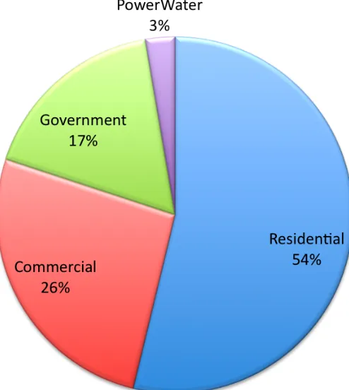
[image:11.595.163.410.286.562.2]The Darwin Region’s water supply system sources its water from both surface water and groundwater sources. Approximately 90 % of water is supplied from Darwin River Dam and the remaining 10 % is supplemented from McMinns and Howard East Borefields. Power and Water Corporation (PWC) is responsible for the supply of potable water to a permanent population of 114,000 people and approximately 50,000 properties including commercial, industrial and government properties, as highlighted in Figure 1-1. The total bulk water consumption in 2009/2010 was 41367 ML and 43,138 ML in 2008/2009. Growth is forecasted to grow at 2-3 % per annum.
Figure 1-1 –Water Consumption by Customer Type (PWC, 2011)
Whilst most cities in Australia have witnessed a sustained reduction in residential water consumption as a direct result of water security threats and ongoing water restrictions, water consumption in Darwin remains well above the national average. In response to this, PWC are currently in the process of developing a Darwin Region Water Supply Strategy. A major focus of this strategy is to review and develop demand management initiatives for the Darwin region. The strategy is supported by the commitment in the Territory 2030 Strategic Plan to reduce water consumption by 20 % by 2015 and a further 10 % by 2025 compared to 2009 consumption levels. (NTG, 2009)
the dry season for an average of 7-8 months. Yearly fluctuations can be up to 10 % and largely depend upon the length of the dry season, transient population cycles and industry cycles. The effects of rainfall and temperature on bulk water consumption for the preceding 5 years are shown in Figure 2-1.
0 20000 40000 60000 80000 100000 120000 140000 160000 180000 1-Ja n-06 27-Ap r-06 22-J un-0 6 17-A ug-0 6 12-O ct-06 7-De c-06 1-F eb-07 31-M ar-07 26-Ma y-07 21-Ju l-07 15-S ep-07 10-N ov-0 7 5-Jan -08 1-M ar-08 28-Ap r-08 23-Ju n-08 18-Au g-08 13-O ct-0 8 08-D ec-08 02-F eb-09 27-M ay-09 22-Ju l-09 16-Se p-09 11-Nov -09 6-Ja n-10 3-M ar-1 0 30-A pr-10 Water Su pply (kL) 0 5 10 15 20 25 30 35 40 D a ily T e mp e ratu re (C) Series2 Series1 Series3
Jan July Jan July Jan July Jan July Jan July
2006 2007 2008 2009 2010
[image:12.595.74.505.137.404.2]340 300 260 240 200 160 120 80 40 0 Da ily Rain fa ll (m m)
Figure 2-1 - Daily Water Production vs. Climate (PWC, 2011)
Residential consumers direct the bulk of water consumption to outdoor uses. Indoor use is also high within the residential sector suggesting that that discretionary garden use is but one factor in explaining the very high rates of consumption in Darwin.
1.4 Justification
Rapid urban and industrial development in Darwin in combination with climate change is contributing to an increased risk and security of supply to the Darwin Water Supply System. While there is a need to secure future water supplies, measures need to be put in place to manage water demand. As demand grows further and annual extraction is increased the available headroom is decreased.
A key component of a future regional water strategy is to implement demand management initiatives to reduce residential water consumption. Reducing water consumption has the potential to defer major capital expenditure on water and wastewater infrastructure. Preliminary forecasting using northern territory water reduction targets in residential households illustrate that the need for the next major water source can be delayed from 2017 to 2024 and beyond if these targets are met. Integrated Supply-Demand Planning (iSDP) is emerging both nationally and
internationally as best practice in the development and analysis of supply and demand options, and PWC are seeking to adopt this framework. End-use measurement is an essential input into the development and assessment of supply side strategies and demand management initiatives.
There is limited information about residential end-uses in Darwin and cities situated in tropical climates. Application of historical end-use models or end use models from other Australian cities cannot be justified without consideration to differences in per-capita demand, demographics, climate and behavioural attitudes to water use.
The disaggregation of residential household water consumption should be considered as the critical first step in the development of demand management initiatives for
residential households. For demand management instruments to be effective, efficient and equitable, their design needs to based on an understanding of how water is used by whom and in what way water savings can be achieved. (Jorgensen et al. 2009)
Diurnal patterns in high irrigating environments are subject to extreme morning and afternoon peaks coinciding with optimum irrigation periods. An understanding of the timing and behavioural influences of end use consumption at peak hour flows, in particular sporadic and automatic irrigation systems, can inform network planning in developing strategies to reduce peak hour flows and therefore reducing water and wastewater capital network infrastructure.
The accuracy of forecasting water use using historical planning estimates for single dwelling residential, medium and high density residential has come under continued scrutiny. The flow on effects from on a under conservative or over-conservative approach to water and wastewater planning can lead to ineffective capital works programs and poor design leading to operational and environmental issues such water quality during non-seasonal flows, increased wastewater retention times, pumping inefficiencies etc.
A pilot study is useful for the testing of new technologies and can identify issues
An end use study undertaken in a tropical climate can highlight extreme trends and variables that may not be evident in studies undertaken in other climatic conditions. A micro-level analysis of end uses over limited number households with ongoing direct contact with the participants can provide insights that may be overlooked from broader analyses.
1.5 Overview of Dissertation
Chapter 2 undertakes a literature review on previous end uses studies and provides case studies for the use smart metering systems to reduce residential consumption. The review focuses on end-uses studies using Trace Wizard software and studies undertaken with significant outdoor use components.
Chapter 3 outlines the methodology undertaken to investigate water consumption in 10 households in Darwin. The chapter defines the technical requirements of the project relating to data capture, transfer, analysis and storage. It develops a model for assessing both indoor and outdoor water uses separately.
Chapter 4 discusses the issues encountered throughout the project and outlines recommendations for future study methodologies.
Chapter 5 provides a summary of overall water use for the 6 week logging period. Chapter 6 investigates indoor consumption and discusses the Trace Wizard process for indoor uses, generates overall indoor use summaries and compares indoor consumption to other studies.
Chapter 7 presents an overview of outdoor water consumption by discussing the methodology of Trace Wizard analysis and investigates the variables that influence outdoor consumption.
CHAPTER 2: LITERATURE REVIEW
2.1 Introduction
The importance of understanding the distribution and variability of end uses of water has evolved with increasing focus to demand management. Water conservation presents a way to economically reduce urban water demands and reduce the need to source future water supplies which are increasing becoming harder to source and considerably more expensive. The shift towards more sustainable and environmental planning has further encouraged the need for water conservation.
Over the past 20 years, advanced end use studies have been undertaken in the United States, Australia, New Zealand, Canada, Spain, Jordan and many other countries. The technological development of data capture, transfer, storage and analysis in recent times have allowed for the ability for water utilities to undertake end use studies in a less intrusive, cost effective and timely manner.
2.2 End Use Measurement
There are a variety of methods used in the collection, transfer and analysis of end use information and usually combine some form of technology with household surveys and/or statistical information. End use measurement can range from manual measurement from house inspections, log books and questionaries to technological measurement using smart meters and data loggers. Data can be transferred for further analysis using manual or automated techniques.
Blokker et al (2010) used a stochastic end use model to estimate residential end-uses in Sydney. The study combined statistical information from census, household surveys and stock appliance manufacturers. Results showed a good correlation to existing end use studies but the approach can lead to inaccuracies, particularly in end uses such as showers and taps. These errors were further highlighted in a study by Mead and Aravinthan (2009) whom undertook a pilot study in Toowoomba and found that estimated manufactured flow rates were different to actual flow rates in household appliances.
Regardless of the level of technology or resolution used in the analysis, surveys and logbooks recording demographic and behavioural data provide an essential link to end-use analysis.
Wide bay water was one of the first utilities to employ smart metering on a broader scale in Australia. The smart meters provided an enhanced understanding of customer water use patterns capable of discerning between overall indoor and outdoor water use and detecting household leakage during off-peak periods. A review by SMEC highlighted the limitations of recording at 1 hour intervals and an inability to disaggregate indoor water use and monitor the effectiveness of end-use scale demand management initiatives. The report recommended for more advanced metering to be applied on a selection of
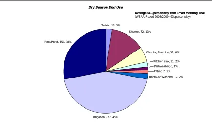
An internal smart metering trial was undertaken on 10 employees from Power and Water using Halytech Wireless Window equipment to monitor water use during the dry (winter) and in the wet (winter) season in 2010. The instruments recorded consumption over a 1 hour period and each household was to record water events with a log audit
spreadsheet. The analyst was required to remotely download the data and estimate water consumption using the water diaries and manufactured flow rates. Results of this study are shown in Figure 1-2. Several of the households could not be disaggregated due the incompletion of water diaries or logger failures. Therefore a key consideration for future studies was to have an independent process that could automatically
disaggregate water use events, minimise household participation and improve data storage and transfer capabilities.
Dry Season End Use
Toilets, 13, 2%
Shower, 72, 13%
Washing Machine, 31, 6%
Kitchen sink, 11, 2%
Dishwasher, 6, 1%
Other, 7, 1%
Boat/Car Washing, 12, 2%
Irrigation, 237, 45% Pool/Pond, 151, 28%
[image:17.595.72.508.230.495.2]Average 541l/person/day from Smart Metering Trial (WSAA Report 2008/2009 493l/person/day)
Figure 1-2 – Previous Internal Smart Metering Trial - Dry Season End Use Summary (PWC, 2010)
2.3 Advanced End Use Measurement
The first version of Trace Wizard software was developed to measure the impacts of a conservation retrofit program in Boulder Colorado and capable of disaggregating end uses from a single water meter (DeOreo et. al 1996). Whilst the system significantly increased the speed and accuracy of flow trace analysis, simultaneous events still required manual manipulation of the database. A further improvement to the software has enabled simultaneous events to be identified within the program and has provided a key link between measured data and end use disaggregation. (DeOreo, 2011).
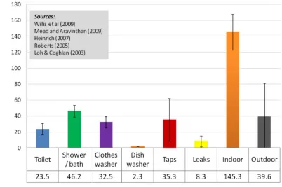
A summary of results for several advanced end-use studies that have utilised Trace Wizard software in recent years is shown in Figure 2-2 (Beal, 2010). The results
Figure 2-2 - Summary of Recent End Use Studies (Beal, 2010)
The majority of indoor water use is directed to showers, clothes washing, toilets and faucet use. Household appliances with distinct volumes and cycles such as clothes washers, dishwashers and toilets show little variance between studies. Faucet use can considerably vary between studies and dependent upon the methodology utilised and the amount of information provided from surveys and water audits. Outdoor water use can considerably vary between regions and the parameters that influence outdoor water use are discussed later.
Several end-use studies have been undertaken in Perth using a variety of approaches to disaggregate end uses. These studies have highlighted the importance of capturing detailed water consumption information in combination to water diaries and surveys; stating that for outdoor irrigation use the respondents could correctly identify the number of irrigation events, however the duration of irrigation events can be
underestimated by as much as 30 % to 50% (Loh & Coghlan, 2003). As Darwin has a high outdoor usage during the dry season, it is imperative that a higher level of accuracy is achieved than capable in a survey-only based approach.
A study was undertaken on 735 single family homes across ten water agencies
for water use and excess irrigation and that this distribution is a key component to designing targeted demand management approaches. . For indoor consumption, the only statistically significant variable was the number of residents in the home and all other variables were random in predicted indoor water use. The study also found that
household income was a much better predictor of water consumption than the marginal prices of water. (DeOreo, 2011)
2.4 Diurnal Flow Patterns
Water consumption varies throughout the day and directly relates with the daily cycles of residents and their interaction with end uses. A typical residential curve applied to a network model is shown in Figure 3-2. A demand multiplier is used to convert average peak day flow to peak hour flows during a peak day scenario. A peak is usually
experienced in the morning and a further peak in the evening and this is when indoor and outdoor consumption is at the maximum. In high irrigating environments, the peak hour factor can considerably increase coinciding with irrigation cycles.
Figure 3-2 - Typical Residential Diurnal Pattern (PWC, 2011)
CHAPTER 3: METHODOLOGY
3.1 Introduction
The methodology for this project is based on methodologies used in previous end use studies. Equipment and software were selected based on similar studies, so in the event of troubleshooting previous or current studies could be contacted for assistance.
The key focus of the methodology was to minimise the reliance of participant
involvement in the study where possible and still be able to achieve outcomes where poor participation arises. Water conservation awareness is lower in Darwin than other regions and therefore the desire to participate in water consumption studies is perhaps lower without the higher exposure to water conservation messages seen in other regions. The methodology also seeks to be as non-intrusive as possible with the aim of observing behaviour without influencing behaviour.
3.2 Sample Selection Process
As a pilot study, a statistically relevant population is not required. However, stratified sampling is essential to providing a realistic sample of the broader population.
Specifications of the acceptable level of error and required confidence limits are not achievable as pilot study.
Selection processes in existing studies generally target higher water users and they are responsible for a higher proportion of water use and where the maximum savings can be achieved. Therefore having a sample above the mean water use of the population is desirable to understand the end use factors that are contributing to higher water use. The study focuses on owner-occupied households as rental households are generally transient and seasonal comparisons become invalid.
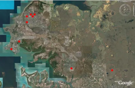
Figure 1-3 - Household Locations
3.3 End Use Equipment
The study required the purchase of 10 new water meters and data loggers for the study. The specifications for each are described below.
3.3.1 Meters
A high resolution of recording is required for flow trace analysis in Trace Wizard. The most common meters used in previous studies is the Actaris CT5-S water meter and are readily available from Australian suppliers. This meter was selected as suitable for this study. Existing water meters in Darwin are generally 20 mm diameter Elster Meters, and therefore a direct switch to the 20 mm diameter Actaris meters was possible without the need for additional accessories. The meter has a long battery life that is suitable for the duration of this study and for the expansion for future studies. The meters are provided with a high resolution reed switch contact closure output.
The meter was modified from its normal 2 pulses / litre to record at 72.5 pulses/Litre at the manufacturing stage. This is currently the highest amount of pulses per litre that can be achieved from a domestic water meter. At the time of ordering these meters have a unit cost of $339.00/unit. The meters were tested during the manufacturing stage. Contractors were sourced to install plugs onto the reed switches.
3.3.2 Data Loggers
Aegis Datacell Rtx data loggers were selected to satisfy the requirements of this study. The logger has a capacity to store up to 2 million records with a battery life of 10 years which combined make it suitable for the duration of this project. The loggers are capable of recording up to 100 Hz which is required for this project. The data loggers are
provided and tested with inserted SIM cards and the setting of all communication and typical operation parameters. SIM cards were purchased locally and sent to Aegis for installation and testing.
The logger was set to record consumption every 10 seconds and to transmit weekly profiles. The logger has remote interrogation and programming capabilities but this could not be achieved with consideration to the sample size and the complexity of IT systems required. Two email addresses were created to ensure a backup of data. Each logger was attached with household abbreviations to ensure transmitted emails could be identified. The emails were staggered in time to ensure identification and minimise traffic.
A software suite was downloaded from the Aegis website to convert the raw data transmitted from the data logger via email to a format suitable for input into Trace Wizard. However, the conversion from the latest version of the software suite could not be achieved and an older version of the software suite was sourced to achieve the conversion. This software was downloaded from the Aegis website.
The loggers were purchased at $900 per unit.
The specification for the Actaris CT5-S water meters are shown in Appendix E.
3.3.3 Pressure Loggers
Pressure loggers were installed at each of the sites and recoded residual pressures over a 5 day period. An average pressure profile was developed for each of the sites. High end irrigation flows were compared against pressures at time of the day. This was necessary as several sites due to the variable nature of pressures throughout the day. One of the pressure loggers recorded erroneous results and pressure for this allotment was compared with nearby pressures and network models.
3.4 Testing and Installation
Data loggers were synchronised to local time. An installation report was generated from each logger to verify correct SIM card installation and signal strength. The data loggers were programmed to transmit an email to check logger settings were correct and operating as expected. Each meter and data logger was labelled externally and serial number recorded to ensure loggers were installed at the correct addresses.
A bracket was developed from Power and Water Personnel to connect the meter to the data logger. The logger is designed to operate in an upright position and this was considered in the bracket design.
The meters and data loggers were installed by qualified Power and Water personnel and contractors over a 4 hour period on 16th August 2011.
Water meters in Darwin are located above ground and therefore careful consideration to operational issues such as environmental damage and security was paramount without affecting the GSM signal strength of the data logger. Most of the water meters were located behind fences or security gates and provided adequate protection.
The bracket orientation needed to be modified in several houses due to proximity near fences. Where meter access was not possible due to plant overgrowth, alternative houses were selected for the study.
3.5 Household Audit and Water Diaries
After the meters and data loggers were in place, a household audit was undertaken on each property over the course of two weeks to provide signature traces of individual water events. The type and rating of each household fixture was noted. Each fixture units was applied for 10 seconds to allow a Trace Wizard profile to be developed for each fixture. This is important as indoor fixtures such as bath taps can be higher than external fixtures and outdoor fixtures during outdoor use can be lower than indoor fixtures. Photographs were taken of each appliance for future reference.
The boundaries of irrigated areas were also determined at the household audit. A household questionnaire was also developed to determine household demographics, water appliances and water use behaviours. This was supplemented with a log book for the first 4-5 days assist in the flow trace analysis in determining dish washer and clothes washer cycles that cannot be determined at the household audit. The log sheets proved to be extremely valuable for complex flow trace analyses particularly on weekends and in identifying common events from the daily cycles of participants.
3.6 Trace Wizard
Trace Wizard is special purpose software used to disaggregate overall water
consumption into individual water uses such as showers, toilets, leaks etc. The program is capable of automatically disaggregating up to two simultaneous events.
Analysis in Trace Wizard is a two part process. The first is to the task of resolving the raw flow trace data from the converted output data logger file into individual water use events. At this stage, the leakage parameters and simultaneous event properties are calibrated. Parameters can be changed to increase the minimum leak tolerance or to adjust properties for the recognition of simultaneous events.
Dishwasher and washing machine cycles can be determined from the household survey. The program provides a fixture library which the analyser uses to select the total number and type of fixtures to cater for each household. The analyser modifies the parameters (e.g. volume, peak, duration and mode) for each fixture to match the individual
household. This is achieved by setting a range of criterion for each parameter i.e. a maximum volume and a minimum volume etc. The order of fixture units in the fixtures library is important as each flow event is matched against the fixture list and assigns a fixture type if the event rests between the maximum and minimum range for all parameters of the fixture type.
Multiple fixtures can be applied for each end use. For example if a clothes washing machine has three cycles of different volumes, peak flow and volumes then each cycle can be matched separately as Clothes Washing 1, Clothes Washing 2, Clothes Washing 3 and the template parameters are set to each cycle. The variation can be minimal and the parameter range can be increased to match all cycles, as long as other household
[image:24.595.70.507.290.546.2]fixtures will not fall within the parameter ranges.
Figure 2-3 - Example Trace Wizard Flow Trace
All water profiles can be viewed in the primary user interface Events Graph. All calculated fixtures are assigned an individual colour for each end use. An example trace wizard flow trace over a 1 hour interval is shown in Figure 3-3. The trace shows two clothes washing cycles, a toilet flush and a simultaneous irrigation event.
Trace wizard calculates three types of events known as base events, trickle event and super events. Trickle events can be automatically incorporated into the previous water event. The interface also allows for water events to be merged or split manually if the water profile does not match the intended water use.
visual inspection. The analyser can then decide whether to modify the existing parameters.
Trace Wizard 4.1 Software had a unit cost of $1495 (US dollars) at the time of purchase.
3.7 Microsoft Excel Database
The template file created as an output from the flow analysis in Trace Wizard is formatted into a Microsoft Access file. The analysed flow traces can be viewed in
Microsoft Access and has several in-built summary queries that summarize the results of the flow trace analysis.
Each weekly flow trace file was exported to Microsoft Excel for increasing graphing and data analysis capabilities. Relevant summaries and queries were generated in the excel files.
Trace Wizard rounds volumes to the nearest 10ml for flow trace analysis and a leakage adjustor script was generated from the raw data to account for differences in low level leakage. Although each event may seem small, the cumulative error from rounding is significant to influence the overall leakage consumption and end use profiles.
3.8 Irrigated Area
CHAPTER 4: PROJECT ISSUES
4.1 Introduction
Only seven of the originally targeted 10 households were successfully used for the result summaries. One of the households was replaced with another household and therefore 8 households were successfully used to generate summaries of results. This chapter
presents some of the issues encountered throughout the course of the project and suggests how these issues can be resolved in future studies.
4.2 Project Issues
• Meter Access
One household had overgrown plant growth and meter access was not possible without significant clearing to gain access and this would endanger the meter installer. It is the responsibility of the homeowner to ensure water meter inspectors can be accessed and read. An additional household was selected to replace this household. This would not have been possible if the target population was random and statistically relevant.
•
Logger Site FailuresAll ten of the data loggers were successfully calibrated, tested and installed in the field. A tampering error message was generated from a data logger on the evening after installation. The data loggers transmitted in excess of 500 emails over the course of a weekend and subsequently drained the battery life of the data logger. The data logger was removed from the household but will likely form part of a future expansion of this study.
• Logger Transmission failures
Data transmission issues were prevalent in the weekly transmission of emails. Only 6 of the 9 data loggers completed successful transmissions over the entire 6 week logger period. The 3 remaining data loggers transmitted 4 emails out of a possible 21 emails. Two of these households are located within a 100 m radius and the 3rd household was
located in a rural area. This indicates that the transmission problems were likely due to poor transmission strength rather than issues with the data loggers. This is an area that will need further consideration in the use of wireless data loggers in future studies. Significant time and resources is required to manually download the data. Two of the data loggers were located inside automatic gates and therefore data recovery needed to be organised outside of working hours. This suggests that sample selection should also consider area transmission strength if possible; however caution needs to be addressed to prevent any bias in water consumers.
Although the study is statistically irrelevant, a household was omitted from the flow trace analysis as it was not representative of the general population and would provide an unrealistic skew on certain end uses.
• Missing Data
Data entries are missing in several households over the 6 week logging period primarily due to logger failures and an inability to recover the information with an on-site manual download. Therefore some statistical summaries could only be generated from complete data sets depending on the type of summary. The variability between weekdays and weekends requires at least weekly cycles to be used and often this could not be reasonably satisfied.
• Resource Expertise
The project required a significant amount of technical requirements and relevant expertise was often difficult to source internally on several occasions. This should be a key consideration for future studies or other water authorities seeking to undertake a smart metering or flow trace analysis. The raw data conservation in particular needed significant external assistance to be achieved.
• Intrusive Nature
The flow trace analysis is extremely intrusive if the analyser personally knows the participants. An effective flow trace analysis requires the analyser to establish daily patterns to correctly identify water events. The more engrossed the analyser becomes in understanding the underlying behaviours of each household end use the more accurate the overall flow trace will be. Simply put, the analyser can understand the daily habits of households better than they know them themselves. For instance, a water diary
indicated that a household had three showers in an evening yet the flow trace only showed two showers events. After querying the householder it was determined that a householder was using the pool as a substitute for the shower and therefore did not appear within the flow traces. These type of insights were numerous.
Future studies should require the analyser to remain anonymous from the participants.
• Complexity of Flow Trace Analysis
The outdoor water use component can provide enough complexity to make it impossible to distinguish individual events. An example flow event is shown in Figure 1-4 which contains several toilet flushes, two showers, bath, faucet use and outdoor irrigation with a continuous leak within the main event.
Figure 1-4 - Complex Flow Trace
• Demographic Bias
The study sample are all water service employees of PWC and therefore would exhibit similar weekly patterns and would be expected to possess a higher awareness of water conservation. It is difficult to extend some of the insights shown in this report to the broader population.
• Further considerations
The following results need to be viewed with caution and should be viewed as an insight only. Although the consumption figures and trends seem realistic for a tropical region, the results may not be relevant to the general population given the statistical bias. There are several considerations to make when interpreting the following results:
¾ The analyser has not undertaken training in Trace Wizard software and the use of the program is self taught using program in-built tutorials.
¾ The analyser had limited understanding of end uses and end use profiles prior to undertaking this assessment.
¾ Most existing studies have at least two people analysing the data to eliminate bias in the results where possible.
¾ Most studies undertake an indoor end use model in the winter (wet) season and use a simplified indoor / outdoor model for summer (dry) season analysis. ¾ Darwin has a much higher water use than most previous studies and may
CHAPTER 5: OVERALL CONSUMPTION
5.1 Introduction
This chapter provides a summary of the results relating to overall consumption over the 6 week logging period. A range of data periods has been used to generate statistical summaries and the data period is indicated for each of the summaries and calculations. There are different variables that influence indoor and outdoor consumption and these summaries are presented separately in Chapter 5 and 6.
5.2 Discussion
The data was collected over a 6 week period from 19th August 2011 to 30th September
2011 for 9 households. One household was omitted from the analysis leaving 8 households available for analysis as discussed in Chapter 4. Overall per capita
consumption estimates were calculated using complete weekly data sets over the 6 week period. Weekly data sets were omitted in several households where data entries were missing and averaged across the remaining weeks, ensuring that an equivalent ratio between weekends and weekdays was maintained. Although not ideal, this methodology was deemed adequate as the variation in consumption between August and September would be minimal and with respect the statistical relevance of the sample population. There were two minor rainfall events witnessed over this period that would likely have a limited affect on water consumption. Statistical summaries were generated from
complete data sets only over the 6 week duration.
The results are presented in average daily water consumption per household measured in terms of litres per household per day (lphh). Average per capita consumption
estimates were generated by averaging all individual per capita estimates measured in litres/capita/day (lpcd) to allow for a direct comparison to other studies. This is
necessary to account for vary degrees of occupancy ratios between regions. Alternatively the results can be expressed in litres per person per day by adding the total consumption for all individual households and dividing by the number of participants in the study. It is important to keep in mind that two methods will produce different values as certain end uses such as leakage and irrigation are not normally distributed.
Statistical summaries for overall consumption were generated from the raw data and the overall indoor / outdoor relationship was developed from the Trace Wizard flow trace analysis.
5.3 Overall Consumption
The only reported figures that can be used as a comparison are annual consumption figures and previous smart metering trials. The variance between overall per capita estimates between wet and dry seasons has been calculated; however the breakdown into leakage, residential, commercial and industrial components is less understood between wet and dry seasons with the variance in climate, transient and industrial cycles.
Average annual residential water consumption for Darwin was 491 KL/household (1345 L/hh/d) from 2008-2009 and 458 (1255 L/hh/d) from 2009-2010. (WSAA, 2011) The average consumption of 1878.1 L/hh/d for the study is higher than these figures which is expected as the study is during the peak consumption period. The variance in wet to dry season for residential properties from the bulk metered data needs further investigation. The overall water consumption divided by the number of participants was found to be 682.9 litres/person/day. This is higher than the previous internal smart metering trail of 541 L/p/d, however the differences in occupancy ratios could not be established. Three complete weeks of data over the six week logging period without missing entries was used to generate statistical summaries shown in Table 1-5. The calculated mean over the three week interval was 1847.3 L which is less than 1878.1 L overall. The 3 week interval is still expected to provide a good indication as to the degree of statistical variance between and within the sample population.
Table 1-5 – Sample Overall Consumption Statistical Summary
Parameter Overall Consumption (L)
Mean 1847.3 ± 1177
Median 1821.8 Maximum 8093.5
The peak daily water consumption for the 3 week statistical analysis for all households was 2650 L/household occurring on Saturday 18th September (n=8). The absolute
maximum consumption for a single property over the logging period occurred on the same day with 8093.5 L. This further illustrates the degree to which individual houses can skew the overall data set and the need for larger data sample than other regions to account for increased variability.
Figure 1-5 illustrates the distribution of overall consumption across the eight households. The figure shows that water consumption is not normally distributed and higher water users skew overall consumption figures. The two highest consuming lots account for 40 % of the total consumption and the two lowest consuming lots account for just 12 % of the overall consumption. The end use contributions to the skewness of water
0 500 1000 1500 2000 2500 3000 3500 4000
1 2 3 4 5 6 7 8
Household Number Av e ra g e Da ily Cons um ption (L) 0% 10% 20% 30% 40% 50% 60% 70% 80% 90% 100% Cum ula tive Cons u m ption (%)
Figure 1-5 - Household Consumption Distribution
Figure 2-5 illustrates the frequency of daily usage for each consumption interval. Figure 3-5 shows the percentage contribution from each consumption interval to the overall consumption. A direct comparison between Figures 2-5 to 3-5 indicates that although the frequency of daily water consumption is higher for lower consumptions the percentage contribution to the overall consumption increases with increasing consumption. For instance, although 80 % of the number of overall consumption days are below 2500 L/day this accounts for 60 % of the overall consumption.
0% 5% 10% 15% 20% 25%
500 1000 1500 2000 2500 3000 3500 4000 4500 More
OVERALL CONSUMPTION (L/DAY - 3 WEEKS)
Re la tiv e Fr eque nc y 0% 10% 20% 30% 40% 50% 60% 70% 80% 90% 100% Cumul a tiv e Fre que n c y
0% 5% 10% 15% 20% 25% 30%
0-500 50
0-10 00 10 00-1 500 15 00-2 000 20 00-2 500 25 00-3 000 30 00-3 500 35 00-4 000 40 00-4 500 Mo re
Overall Daily Consumption (Litres)
% of O v e ra ll Cons um ption b y inter v a l 0% 10% 20% 30% 40% 50% 60% 70% 80% 90% 100% C u mu lat ive % by Int e rv al
Figure 3-5 – Percentage Contribution to Overall Consumption per Interval
A higher proportion of water use is used on weekends than on weekdays coinciding with increased indoor and outdoor consumption. The mean water consumption on weekends was 2248 l/hh/d over the 6 week logging period which is higher than the average weekday consumption of 1736 L/hh/d. The end use contribution to weekends and weekdays are shown in Chapter 5 and Chapter 6.
5.4 Trace Wizard Analysis – Overall Consumption
A flow trace analysis was undertaken for two of the six weeks to provide a highly detailed end use breakdown for each of the 8 households. The average household consumption was determined to be 1881 L/hh/d which is slightly greater than the overall mean of 1871 L/hh/d.
As previously mentioned, the selection methodology for two average weeks were not continuous and therefore the results for each indoor and outdoor end uses will contain bias. It can be observed that the pool filling events significantly increase daily
consumption and selection of two average weeks were generally outside of observed pool filling events. However, for the purpose of providing an insight into water
consumption this methodology is adequate. An extended flow trace analysis is required to account for the variability of pool filling events on overall consumption and increase confidence in the results.
OUTDOOR CONSUMPTION, 1447 L/Day
77%
INDOOR CONSUMPTION, 434 L /Day
23%
Figure 4-5 – Overall Indoor / Outdoor Consumption per household.
CHAPTER 6: INDOOR CONSUMPTION
6.1 Introduction
Indoor use comprises 23 % of the total consumption for the eight households. This chapter discusses the approaches and limitations of the Trace Wizard analysis, overall indoor use summaries and compares indoor use to other end use studies
6.2 Trace Wizard Summary- Indoor Water Use
6.2.1 Clothes Washing
Clothes washing events have a distinct number of cycles, volumes, flow rates and durations and can be easily identified within a flow trace. Often, simultaneous events prevent the template from identifying the trace however a least one cycle is usually identified. The remaining cycles can be identified with consideration to the peak flow rate, volume and duration of other cycles. Six out of the eight households possessed top loading washing machines with only two of the households with front loader washing machines. Front loader washer machines are considered to be more water efficient than top loading machines and use approximately half the total water use per cycle than top loaders. An example clothes washing flow trace is shown in Figure 1-6.
Figure 1-6 – Front Loader Clothes Washing Cycle
6.2.2 Dish Washing
least one cycle and the other cycles can be determined from the durations between cycles. Five of the eight households had dishwashers. Two of these households never used the dishwasher during the two week flow trace analysis.
Figure 2-6 - Dishwasher Flow Trace
6.2.3 Showers
Figure 3-6 – Shower Flow Trace
6.2.4 Toilets
Two different toilet profiles can be observed within Trace Wizard. Toilets with a long tail can be easily determined and generally have a high initial flow rate and reduces as the cistern fills up. Figure 4-6 shows an example toilet flow trace, and shows several leakage events following the toilet event. Depending on the household, two separate fixtures can be allocated to account for half flush and full flush events.
Figure 4-6 – Toilet Flow Trace
6.2.5 Leakage
Leakage can be divided in two categories consisting of continuous and discrete leakage. Parameters in Trace Wizard need to be altered to separate continuous leakage from other events; otherwise all events will be classified as simultaneous events. For example, a simultaneous shower and toilet leakage will assign the entire event as shower. The two events cannot be separated as the cause of the leak maybe directly related to
simultaneous end use or the leak may reduce due to a reduction in pressure.
Figure 5-6 – Leakage Flow Trace
6.3 Discussion
A flow trace analysis was undertaken on 2 average weeks of the 6 week data set. The limitations and bias of this method were previously explored in Chapter 4 and 5. It is expected a more accurate assessment can be undertaken in the wet (winter) season where the bulk of water consumption will be indoor consumption. The results presented in this chapter provide an insight into indoor water consumption and statistical
summaries focus on overall volumes from each end use.
Statistical summaries are expressed in terms of average per household use (L/hh/d) by taking the average of individual indoor household consumption and averaging across the eight households. Average per capita estimates (L/p/d) were calculated by taking the average of each individual per capita estimate across the eight households.
Average per capita estimates is the preferred method to compare to other regions to account for varying degrees of occupancy ratios between regions. There are several factors that need to be considered when interpreting these results. The number of visitors and guests residing at infrequent intervals at several of the households was impossible to track. This is typical of the dry season as this is the ideal time to visit. Therefore per capita consumptions would be expected to be higher in the dry season that the wet season to account for the increased number of visitors assuming internal usage from the participants is the same. In addition, the frequency of each end use would increase to account for the increased number of visitors.
6.4 Overall Indoor Summary
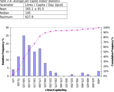
[image:40.595.75.465.228.545.2]The average indoor use over the two week flow trace analysis for each household was 432.9 L/hh/d. This equates an average indoor per capita consumption of 165.1 l/p/d. The average occupancy ratio in the study is 2.75 which is slightly higher than the 2.5 occupancy ratio for Darwin. (ABS, 2010). The highest average per capita consumption was 627.9 lpcd on a Saturday with 72 % of the daily consumption directed to clothes washing. This matched the highest peak day from a household with 1256 L in a single day. The 95 % confidence level for indoor litres/capita day is 17.1 L over the two week period.
Table 1-6- Average per Capita Indoor Statistics
Parameter Litres / Capita / Day (lpcd) Mean 165.1 ± 91.5
Median 145 Maximum 627.9 0 5 10 15 20 25 30 <75 75-100 1 00-125 1 25-150 1 50-175 1 75-200 2 00-225 2 25-250 2 50-275 2 75-300 3 00-325 3 25-350 3 50-375 3 75-400 4 00-425 4 25-450 >45 0 Litres/Capita/Day Relat ive Frequenc y % 0% 10% 20% 30% 40% 50% 60% 70% 80% 90% 100% Cu mulat ive Freqency %
Figure 7-6 - Frequency distribution of indoor daily per capita water use
The frequency distribution of indoor daily per capita water use is shown in Figure 7-6. The most frequency indoor consumption was between 100 – 125 L/p/d. A standard variation of 91.5 lpcd or 55 % indicates an extremely high variation in indoor water consumption and a high positive skew of 2.73. The skew is primarily a result of a much higher indoor water use on weekends.
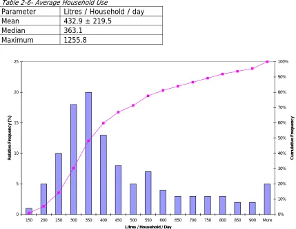
Table 2-6- Average Household Use
Parameter Litres / Household / day Mean 432.9 ± 219.5
Median 363.1 Maximum 1255.8
0 5 10 15 20 25
150 200 250 300 350 400 450 500 550 600 650 700 750 800 850 900 More
Litres / Household / Day
Re
la
ti
v
e
Fre
que
nc
y (%)
0% 10% 20% 30% 40% 50% 60% 70% 80% 90% 100%
Cumulat
iv
e
Fre
que
ncy
Figure 8-6 - Indoor Household Consumption Distribution
6.5 Disaggregated Household Use
15.9%
36.5%
13.5% 20.6%
1.0%
12.5%
LEAK
SHOWER
TOILET
CLOTHES
DISHWASHER
[image:42.595.132.417.85.318.2]FAUCET
Figure 9-6 – Percentage overall indoor end use volumes.
Shower use contributes to a highest percentage with 36.5 % of the overall consumption followed by 20.6 % for clothes washing. Leakage is high with 15.9 % of the total
consumption. Toilet use contributes to 13.5 % and faucet with 12.5 %. Dishwashing consumption was minimal with 1 % of total indoor use.
Although not included in the study, the ninth household had a major leak which would have further increased the leakage percentage if included.
The statistical summaries for average per capita end use consumption are shown in Table 3-6. Note that the overall household percentages for each end use are different that than calculate average per capita percentages. This is because water consumption does not follow a normal distribution. End uses such as irrigation, leaks, dishwashing generally have a high variation where else end uses such as showers, clothes washing, toilets and faucets are common end uses and subject to less variability.
Table 3-6 – Average per Capita Statistical Summary
Parameter Leak
(L/p/d) Toilet (L/p/d) Clothes Washing (L/p/d)
Shower
(L/p/d) Dish Washer (L/p/d)
Faucet (L/p/d) Mean 28.9 23.4 35.5 53.7 1.9 21.0 Median 7.7 18.4 20.3 52.8 1.1 22.4 Standard
Deviation 34.6 16.6 16.6 19.5 2.3 8.3 Maximum 78.0 55.7 114.9 78.7 5.5 31.7
0% 10% 20% 30% 40% 50% 60% 70% 80% 90% 100%
1 2 3 4 5 6 7 8
Household Number
% Contribution
Shower
Clothes Washing
Faucet
Toilet
Dishwasher
[image:43.595.83.505.79.325.2]Leak
Figure 10-6 - Indoor Water Consumption Profiles for Individual Households
Figure 10-6 shows that the majority of leakage is occurring within three households and exceeds 50 % of the total indoor consumption for one household. Two of the three leakage events were related to outdoor irrigation systems and the other significant leak was attributed to a toilet. Two of these households participated in a previous smart metering trial last year and were notified of the leak during the previous trial. One of these households did not fix the leak during that time, but when shown the percentage contribution of leakage to overall consumption the participant was more willing to fix the leak. This supports the use of visual pie charts as an effective tool in motivating
individuals to reduce leakage. The other household rectified the leak during the previous smart metering trail; however this study indicates that a further leak has developed during the past year. The sample size is too small to extrapolate to the broader
population, but given that the ninth household also possessed a major leak the results indicate that household leakage could be a widespread issue.
Shower use is also skewed towards several households as demonstrated in Figure 10-6. It can be observed that the influence of previous exposure to water restrictions had an effect on percentage shower consumption for each of the households. Interstate
residents with previous exposure to water restrictions used less than residents who have never been exposed to water restrictions. It could also be observed in the flow trace analysis that interstate residents are more likely to exhibit water efficient practices such as reduced shower durations and faucet use. This can not be conclusively illustrated due to the sample size.
6.6 Comparison to other studies
In Australia, most of cities analysed have previously faced water security threats and the populous have been subject to water conservation programs and water restrictions. The majority of residents, in particular Darwin locals, have generally not been exposed to water restrictions or been subject to significant water conservation initiatives. Table 4-6 and 5-6 compares the average per capita consumption and average percentage consumption for indoor uses to other regions in Australia. The results highlight that there is limited variability in indoor water consumption from this study to most other end use studies even with the range of climate and behavioural variables. The sample limits extrapolation and may not be indicative of the broader population. Leakage is high with comparison to other studies and potentially influenced by the age of the properties in the analysis. However given that most of the houses have been part of previous in-house smart metering trials and leakage is still high, this suggests it is possibly a widespread occurrence.
Table 4-6 – Average per capita consumption for each end use (L/p/d)**
Region Leak
(L/p/d) Toilet (L/p/d) Clothes Washing (L/p/d)
Shower
(L/p/d) Dish Washer (L/p/d)
Faucet (L/p/d) Darwin (n=8) 28.9 23.4 35.5 53.7 1.9 21.0 South East
Queensland (n=252)
6.0 16.5 31.0 44.5 2.5 27.5
Toowoomba
(n=10) 0.5 14.2 25.4 48.7 2 16.8
Melbourne
(n=100) 15.9 30 40 49 2.7 27
Perth (n=120) 21 27 33 83
Auckland
(n=50) 7.0 31.3 39.9 50.4 2.1 22.7
Table 5-6 Average percentage of total consumption**
Region Leak Toilet Clothes
Washing Shower Dish Washer Faucet Darwin (n=8) 15.9 13.5 20.6 36.5 1.0 12.5 South East
Queensland (n=252)
6.0 16.5 21.0 30.5 2.0 19.0
Toowoomba
(n=10) 0.4 12.3 22.7 45.2 2.1 16.8 Melbourne
(n=100) 6.0 13.0 19.5 23.0 1.0 12.0 Perth (n=120) 10.0 13.0 16.0 7.0 Auckland
CHAPTER 7: OUTDOOR CONSUMPTION
7.1 Introduction
Outdoor use contributes 77 % of the overall consumption for the eight households and therefore an increased focus has been placed on understanding the variables that influence outdoor water use than indoor water uses. This chapter presents an overview of the Trace Wizard analysis for outdoor uses, generates statistical summaries and discussion for outdoor water use and investigates the relationship between lot size, irrigated area and outdoor consumption.
From the household surveys and flow trace analysis it is clear that the mentality and activities surrounding irrigation events is closely correlated to the dry vs. wet season interaction. It is not a question of if it will rain, but a question of when it will rain.
7.2 Trace Wizard Summary – Outdoor Water Use
7.2.1 Irrigation
[image:45.595.70.508.502.758.2]Irrigation can be separated into automatic or sporadic irrigation events. Automatic events are controlled by a timer and can have several cycles up to 10-15 minute duration per cycle over multiple cycles. Figure 1-7 shows an automatic irrigation event with 9 cycles over a 1 hour duration with varying durations. This corresponds to 9 separate irrigation zones on the property and each volume and flow rate of each cycle is dependent on head losses, amount of irrigated area and the required application ratio for each zone. These events are easy to recognise and simultaneous events can be identified through changes to the irrigation profile.
Sporadic irrigation events are extremely variable in nature and can vary between long sustained flow rates from rose head sprinklers to relatively short events such as car washing. A boat washing event can be seen in Figure 2-7. Consideration to the time of the day, the peak flow rate, frequency of event, water diaries and surveys provide sufficient information to assess sporadic irrigation events. Indoor events such as rinsing dishes can easily be mistaken with outdoor events and vice versa for fixtures with similar flow rates. Therefore there will a degree of error related to faucet use and outdoor use for these properties.
Figure 2-7 – Example Outdoor Boat Washing Event Flow Trace
7.2.2 Pools
Outdoor use has not been divided into irrigation and pool events due to the selection methodology and the limited sample period for flow trace analysis as highlighted in Chapter 4. There are however a number of observations that can be noted and are discussed here.
Pool events can usually be identified from extremely long events over several hours, however often sporadic irrigation events can reach similar durations and posses a similar flow rate. There are a number of ways these events can be separated. For instance, excessive daily consumptions usually indicate that a pool event has occurred in
Figure 3-7 – Example Pool Event Flow Trace
A reduced number of pooling filling events were observed in the raw data where pool covers, sails and tree cover were present on the property.
7.3 Overall Outdoor Summary
[image:47.595.73.504.67.321.2]Outdoor water consumption has a closer correlation to lot size or irrigated area than number of residents per household. Therefore the results for outdoor use are expressed using these parameters only. All the participants in the study were irrigating over the 2 week flow trace analysis.
Table 1-7 – Lot Size Statistics
Parameter Lot size (m2)
Mean 4519 ± 10338 Median 817 Maximum 30100
The average lot size in the sample population is 4519 m2 with a median of 817 m2. The
rural property in the data set is contributing to an extremely high skew with a maximum of 30100 m2. The lot size on seven of the eight properties is well below the calculated
mean and this scenario would not be demographically relevant to the broader
population. Therefore a relationship between lot size and overall consumption cannot be adequately represented. The lot sizes were determined from Facility Information Systems and were modified to include front road verges.
Table 2-7 – Outdoor Water Use Statistics
Parameter Daily Outdoor Water Use (L/hh) Average 1447 ± 1169
[image:48.595.72.486.205.457.2]Median 1419 Maximum 7340
Figure 4-7 illustrates how higher water users use a much higher percentage of outdoor water use than lower water users. The highest water user accounts for over 26 % of total outdoor water use across the eight households.
0 500 1000 1500 2000 2500 3000 3500
1 2 3 4 5 6 7 8
Houshold Number A ver