Hierarchical Bayesian modelling of gene expression time series across irregularly sampled replicates and clusters

R E S E A R C H A R T I C L E

Open Access

Hierarchical Bayesian modelling of gene

expression time series across irregularly

sampled replicates and clusters

James Hensman

, Neil D Lawrence

and Magnus Rattray

Abstract

Background: Time course data from microarrays and high-throughput sequencing experiments require simple, computationally efficient and powerful statistical models to extract meaningful biological signal, and for tasks such as data fusion and clustering. Existing methodologies fail to capture either the temporal or replicated nature of the experiments, and often impose constraints on the data collection process, such as regularly spaced samples, or similar sampling schema across replications.

Results: We propose hierarchical Gaussian processes as a general model of gene expression time-series, with application to a variety of problems. In particular, we illustrate the method’s capacity for missing data imputation, data fusion and clustering.The method can impute data which is missing bothsystematicallyandat random: in a hold-out test on real data, performance is significantly better than commonly used imputation methods. The method’s ability to model inter- and intra-cluster variance leads to more biologically meaningful clusters. The approach removes the necessity for evenly spaced samples, an advantage illustrated on a developmental Drosophila dataset with irregular replications.

Conclusion: The hierarchical Gaussian process model provides an excellent statistical basis for several

gene-expression time-series tasks. It has only a few additional parameters over a regular GP, has negligible additional complexity, is easily implemented and can be integrated into several existing algorithms. Our experiments were implemented in python, and are available from the authors’ website: http://staffwww.dcs.shef.ac.uk/people/J. Hensman/.

Background

Gene expression time course experiments have been used to investigate fundamental biological processes which are often dynamic in nature. For example, the cell cycle [1], cell signalling [2], circadian rhythms [3] and developmen-tal processes [4] have been studied extensively using gene expression time-series data.

Many computational approaches to time-series analysis are not always well suited to gene expression data, where missing measurements are common and time points may

*Correspondence: [email protected]; [email protected]

1Department of Computer Science, The University of Sheffield, Sheffield, UK 3Faculty of Life Science, The University of Manchester, Manchester, UK Full list of author information is available at the end of the article

not be spaced regularly. In many conventional time-series models such as state-space models [5,6] there is no straightforward manner to deal with missing data, and time points must occur at regular intervals. Whilst gene expression experiments can be sampled regularly, such designs may not be optimal from a statistical or cost perspective. A method for modelling arbitrarily sampled time points may elicit more information from fewer sam-ples, where time points are selected to capture pertinent temporal features.

Furthermore, existing time-series models do not neces-sarily capture thestructureof gene expression data. Many gene expression time-series are performed with multiple biological replicates: the crude method of simply aver-aging the replicates may be discarding interesting infor-mation. It is also unclear what to do when the replicates

are not sampled at the same times. There is a need for a temporal model which deals with the replicate structure.

Our proposed model is based upon two important ideas: Gaussian process (GP) regression allows for parsimo-nious temporal inference, whilst a hierarchical structure accounts for (temporally structured) covariance between biological replicates. Additional layers can be added to the hierarchy to model more structure in the data. For example, in a data fusion application, a layer of hier-archy can be used to account for differences between gene expression measurement platforms; or in a clus-tering application, a hierarchical layer can be added to account for temporal covariance of genes within a cluster.

GPs have been successfully applied to the analysis of gene expression time series by several authors [7-9]. There is little doubt that they provide a coherent and princi-pled framework for regression: for an introduction see [10]. Our contribution is to proposehierarchicalGaussian processes to deal with structure in the data. We pro-vide an introduction to the idea, deriving a novel covari-ance function which accounts for structure. The idea is simple to implement yet highly effective as we demon-strate on several problems. A hierarchical GP model could easily be integrated with existing GP-based appli-cations, allowing them to properly account for replicate structure.

In a further contribution, we manipulate the marginal likelihood expression for the hierarchical GP model for the case where each part of the structure is sampled at the same time, leading to an expression with reduced compu-tational complexity. This situation is most likely to occur during clustering of genes, which must all be measured simultaneously using high throughput methods.

Short time series are prevalent in gene-expression data sets [11]. Our GP-based model is well suited to short time-series, and the behaviour of GPs can be set to mimic that of other temporal models (such as autoregressors) through the covariance function [10], though in this work we use a simple form for the covariance which assures smoothness of the underlying dynamics.

Unlike other time-series based approaches, GPs are not restricted to data which has been sampled at evenly spaced time points. The model therefore removes any restriction on temporal sampling — it can be totally irreg-ular and differ between replicates. This also allows our method to deal with both randomly and systematically missing data. We show how the model can be used for data fusion where the temporal sampling differs between experiments.

Related work

Hierarchical models are an important idea in Bayesian statistics [12], allowing information to be exchanged

between related groups of data. The idea is that by per-forming inference on the structure as a whole, rather than on each part of the structure independently, infer-ence is improved. GPs have been successfully used in models of gene expression time-series before; for exam-ple for inferring transcriptional regulation [8], and to identify differential expression in time-series [7,13]. A key contribution of this work is to combine hierarchical structures with GPs to provide a parsimonious and ele-gant method for dealing with replicated gene expression time-series.

An alternative to our method was proposed by [14]. In this model, uncertainty is assumed in the time of data collection, and the time-shift in each replicate is esti-mated. In our model, the times are assumed correct whilst the shift is assumed to occur in the expression. Our model has significant computational advantages, since we can marginalise the shifts in expression analytically under the GP framework, whilst the method proposed in [14] required optimisation of a large number of vari-ables (one for each observation). Further, our model is easily included in more complex GP-based models, such as the clustering application which we shall demonstrate. The estimation of time-shifts would be difficult to incor-porate into a clustering method, especially considering the very large numbers of parameters which require optimising.

Clustering expression data while modelling within-cluster variance is one of the primary applications of our model. Previously, [15] proposed a random effects model to account for variance between observations of genes and also within clusters of genes. Further, [16] and [17] explored clustering methods with hierarchical structures to model replicate variance. In these models, replicate variance was modelled as multivariate Gaussian around some gene-specific mean, and the gene’s expres-sion was considered multivariate Gaussian around a cluster-specific mean. This paper presents a similar but more powerful idea: we use a hierarchy of GPs to model gene-specific and replicate-specific temporal covariance. We demonstrate that the introduction of a GP prior makes inference of clusters more viable by reducing the num-ber of parameters required to model the data within a cluster, and we also provide a method for dramatically reducing the computational cost of evaluating clusters under our model. Previous methods for clustering tem-poral data (e.g. [18]) have not used the replicate structure in the model.

Methods

Background: Gaussian processes

briefly introduce GP regression and introduce some nota-tion: for an in-depth introduction one may consult [10].

To perform regression using GPs, we adopt a Bayesian approach. Starting with a priordirectly over functions, we update the distribution in light of observed data, mov-ing to a posterior distribution. Usmov-ing standard results for Gaussian distributions, regression involves only some simple linear algebra. The GP prior is fully specified by two functions, a mean function m(t) and a covariance functionk(t,t), and is denoted

f(t)∼GPm(t),k(t,t). (1)

For practicality, a zero-mean function is often assumed; throughout this work, the squared-exponential covariance function will be used:k(t,t)=αexp{−γ (t−t)2}.

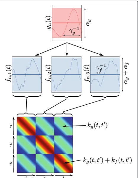
Our choice of covariance functions represents a prior belief that the underlying functions are smooth. Other covariance functions could be selected using a model-selection procedure [10]. The parameters of the covari-ance function (referred to as hyper-parameters) control the amplitude (α) and relative length-scale (γ) of the func-tions (see Figure 1 for an illustration). The form of the covariance function captures a very simple assumption about the function: that function points which are close to each other (t−tis small) are highly correlated, whilst points which are distant(t−tis large) are less correlated. Regression can be performed by using the marginal and conditional properties of multivariate Gaussian distribu-tions. Supposing we have observationsfof a function at timest, and wish to predict the values of that function at timest, which we denotef: the joint probability offand

fis given by

p

f f

=N

f f 0,

Kt,t Kt,t Kt,t Kt,t

, (2)

where the covariance matrix Kt,t has elements derived from the covariance functionk(t,t), such that the(i,j)th

element ofKt,tis given byk(t[i] ,t[j]). Consistency of the GP means that it is not necessary to consider the values of the function where we do not have data: these val-ues are trivially marginalised. To perform regression, the conditional property of the multivariate Gaussian gives:

p(f|f)=N f|Kt,tK

−1

t,tf,Kt,t−Kt,tK

−1

t,tKt,t

.

(3)

In practice, we are presented with a measurement vec-tory which is a noise corrupted version off. Assuming Gaussian noiseait is possible to writep(y|f)=N(y|f,βI), whereβis the variance of the noise andIthe appropriately sized identity matrix, and then marginalise the variable f. Equivalently, one can consideryto be observations of

Figure 1An illustration of a simple hierarchical GP.Top: the prior over the underlying functiongn(t), with the meanμ(t)=0 shown as

a heavy solid line, and the shaded area representing the variance (amplitude) of the function, controlled by the hyper-parameterαg. A

single sample from the prior is shown as a narrow line, and the length-scale of the function, inversely controlled by the

hyper-parameterγg, is marked. Middle: three functions, representing

three replicates are shown, along with samples conditioned on the sample shown ingn(t). The three replicates follow the trend ofgn(t),

but deviate independently by a small amount (varianceαf) with a

short length-scale, marked in the third replicate. Bottom: the covariance matrix used to generate the samplesn. Note the

block-wise relationship to the replicates.

the Gaussian process y(t), whose mean function is the Gaussian process f(t), and covariance function isβδ_t,t. This hierarchical structure is used later in this publica-tion to build GP priors over replicates and clusters. Either interpretation gives a joint density:

p

y f

=N

y f 0,

Kt,t+βI Kt,t Kt,t Kt,t

(4)

and regression follows from the conditional property sim-ilarly to (3).

significant attraction of the method is that this occurs in closed form as (3). However we must still deal with hyper-parameters of the covariance function. Here, we make use of the usual technique which is to optimise the hyper-parameters using type-II maximum likelihood. That is, collecting the hyper-parameters α,β and γ in to a vec-tor θ, we use gradient methods to optimisep(y|θ) with respect toθ. This is given by

logp(y|θ)= −D

2 log 2π− 1 2

×log|Kt,t+βI| − 1 2y

_[Kt

,t+βI]−1y, (5)

which depends onθthrough the covariance matrixKt,t. A hierarchy across replicates

Gene expression time-series may be collected in multiple replicates, to account for biological variation. The idea is that there exists some common trend, present in all repli-cates, which we wish to identify, and the measurements made of each replicate vary due to biological differences as well as technical noise.

We shall use the notationynr to denote the vector of

measurements of gene expression of thenthgene, in the rthbiological replicate; these measurements were made at times which we collect into a vectortnr. The data for the

nthgene is denotedYn= {ynr}Nnr=1,Tn= {tnr}Nnr=1.

Our proposed methodology mimics the structure of the data, directly modellingunderlyingtime-series as well as the biological variation, and accounting for (uncorrelated) measurement noise. First consider a time-series model of a single gene. To combine replicates of a particular gene’s time-series, we use a Bayesian hierarchical approach: the underlying expression profile of thenthgenegn(t)is

pre-sumed to be drawn from a zero-mean GP with covariance kg(t,t), whilst the expression profile of a particular

repli-catefnr(t)is drawn from a GP whose mean isgn(t). Thus

gn(t)∼GP

0,kg(t,t)

, fnr(t)∼GP

gn(t),kf(t,t)

. (6)

Note that the two covariance functionskgandkf may in

general be different: we have used the squared exponen-tial function for both, with independent parameters. This simple model is illustrated in Figure 1, where the depen-dent nature of the functions is illustrated, as well as the effects of the hyper-parameters.

The elegance of the hierarchical approach lies in its lin-earity: it is simple to show that two points on the function

fnr(t)are jointly Gaussian distributed with zero mean and

covariancekg(t,t)+kf(t,t). Furthermore, two points in

separate replicates are jointly distributed with covariance kg(t,t). Thus, given a set ofNnreplicates of gene

expres-sion time-series for a particular gene,Yn= {ynr}Nnr=1, taken

at different time pointsTn= {tnr}Nn_r=1it is possible to write

the likelihood:

p(Yn|Tn,θ )=N

ˆ

yn|0,n

, (7)

whereyˆnhas been used to denote the concatenation ofYn, ˆ

yn =[yn,1,yn,2. . .yn,Nn],θ represents the parameters of

the covariance functionskg andkf, and the block ofn

corresponding toynr,ynr is given by

n[r,r]=

Kg(tnr,tnr)+Kf(tnr,tnr)+βI ifr=r

Kg(tnr,tnr) otherwise.

(8)

In order to make inferences about the functions gn(t)

and fnr(t), the covariances between the data Y and the

functions are required. Using the superscripted y(t)nr to

denote the element ofynrobserved at timet:

cov y(t)_nr,gn(t)

=kg(t,t), (9)

cov y(t)_nr,fnr(t)

=

kg(t,t)+kf(t,t) ifr=r

kg(t,t) otherwise.

(10)

Inferences about functions can then be made using the standard methods described above, and hyper-parameters of the covariance functions can be optimised.

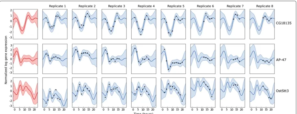
Fitting a hierarchical model to a set of replicates can be used as a diagnostic tool. In particular, by exam-ining the maximum-likelihood values of the covariance function parameters, we can assess how noisy the exper-iment is, and how similar the replicates are. Figure 2 shows three examples of hierarchical regression of the time course data described the Results section, for three genes (modelled independently), with each gene shown in one row in the figure. The leftmost panes in the figure show the inferred function for the gene,gn(t), and

subsequent panes show the inferred functions for each replicate,fnr(t).

These examples demonstrate different behaviours of the time-series which are captured by the model. For the first gene, CG18135, the replicates are quite similar, and most deviation of the data fromgn(t)is attributed to noise. The

under-Figure 2Hierarchical GP regression on the expression of three illustrative genes during Drosophila Melanogaster development, using eight replicates with different time sampling.Each row represents one gene. The leftmost panes show the inferred functiongn(t), subsequent

panes represent the replicates. Solid lines show the mean of the predicted function, and the shaded area represents the 95% confidence interval. The parameters of the covariance function were optimised by maximum likelihood. Note that the replicates contain different numbers of data and different times.

lying functiongn(t), and only 6% each to replicate variance

and noise, i.e. the model ‘recognised’ the similarity of the replicates.

The gene represented by the middle row is AP-47, and it can be seen that there is considerable replicate variance: although each replicate follows a similar pattern, the pat-tern is ‘amplified’ differently in the replicates. Here, the model attributes 60% of the data’s variance to the function gn(t)and 34% tofnr(t), with 6% to noise.

The gene represented by the bottom row of Figure 2 is OstStt3. Here, the variances of gn(t), fnr(t) and noise

are 55%, 36% and 8% respectively. The model recog-nises the differences in the replicates, but uses a long length scale for fnr(t). In this gene, the detailed

pat-tern of the time-series is captured entirely by gn(t),

and fnr(t) is used to account for amplitude shifts

between replicates. Note that these cannot be simply ‘nor-malised out’ because not all replicates cover the same temporal region. These genes were selected using a sim-ple filtering procedure. The model was fitted indepen-dently to each gene on a microarray, and the genes were ranked according to the ratio of signal variance (a hyperparameter ofkg) and replicate-plus-noise variance

(hyperparameters fromkf).

Deeper hierarchies

In many cases, gene expression time-series may have more structure than simply biological replicates. For example, we could incorporate previous studies in a hierarchical fashion. In general, suppose that there is some underlying functiongn(t)which models the general gene expression

activity for thenthgene. Subsequently, we define the func-tionseni(t)for each experiment which we want to model,

and finallyfnir(t)for the rthreplicate in the ithexperiment.

gn(t)∼GP

0,kg(t,t)

, eni(t)∼GP

gn(t),ke(t,t)

, fnir(t)∼GP

eni,kf(t,t)

.

(11)

With every layer of the hierarchy, we have introduced new parameters corresponding to the covariance function for that layer. Note that the hierarchy can be extended arbitrarily to represent the structure of the data. For exam-ple, we might want to model biological variation where the lineage is known, or to model inter-species variation, or to build a hierarchy which reflects the phylogenetic relationship between species.

An efficient model of clusters

Clustering of gene expression time-series is often per-formed with a view to finding groups of co-regulated or associated genes. The central assumption is that genes which are involved in the same biological processes will be expressed together: they share an underlying time-series.

In order to model a group of genes as defined by a cluster, the hierarchical model is extended to a three-layer hierarchy across the cluster, individual genes and replicates.

All genes in the ith cluster are presumed to share an underlying profilehi(t), and subsequently each gene

a profile fnr(t). The mean of each level in the hierarchy

is given by the level above, so the dataYi in cluster iis

modelled by:

hi(t)∼GP0,kh(t,t)

, gn(t)∼GP

hi(t),kg(t,t)

, fnr(t)∼GP

gn(t),kf(t,t)

.

(12)

If yˆi is the concatenation of all of the yˆn representing

genes in theithcluster, noting that eachyˆnis itself a

con-catenation of the biological replicates, then the marginal likelihood of the expression data in theith cluster,Yi is

given by

p(Yi|Ti)=N

ˆ

yi|0,i

(13)

where the covariance matrix_iis structured such that the block corresponding to the two genesnandnis given by

i[n,n]=

n+Kh(tn,tn) if n=n

Kh(tn,tn) otherwise. (14)

Note that the diagonal blocks of_iarethemselves block-structured, reflecting the double hierarchy in the model.

The computational complexity of this model grows cubically as the size of the cluster increases, which is an undesirable property. To reduce the computational load, it is possible to exploit a known property of the data. In each array all genes are simultaneously measured, although we allow different times for each replicate. Denoteˆtthe con-catenation of the times in all replicates, defineKhas the

covariance matrix formed by evaluatingk_hon the grid of

ˆ

t, andna covariance matrix structured as (8), modeling

the variance of a single gene. The marginal likelihood can then be written

p(Yi|Ti)=2π− NiD

2 |_Kh|

1

2|_n|Ni2|K_h−1+Nin|

1 2

exp{−1₂{

Ni

n=1

y_nn−1yn−Ni2y¯in−1(K−h1+n−1)−1n−1y¯i}},

(15)

where y¯i is the mean of the yˆn in the cluster, D is the

length oftˆ, andNi is the number of genes in the

clus-ter (see appendix for a derivation). This expression has reduced the computational complexity of the model from

O(N_i3D3)toO(D3).

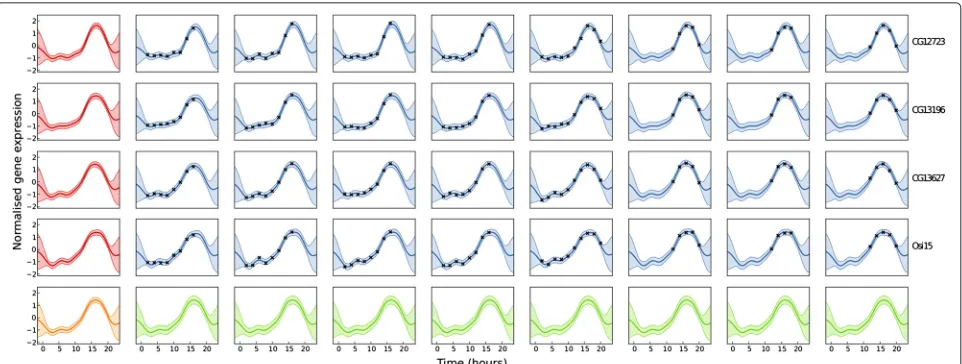
An example of this model is shown in Figure 3. The inferred functionh(t), shown in the bottom-left pane has a single wide peak at around 15 hours; all of the functions gn(t)(leftmost column) show a similar pattern, though the

functions are each ‘distorted’ a little, with the width of the peak varying from gene to gene. Similarly, each replicate shows a similar pattern to the mean function for the cor-responding gene, with smaller variations. The bottom row shows the predictive density for a new gene within the cluster.

Clustering

To use our model for clustering, the partitioning of genes into clusters needs to be inferred. Dunson [18] proposed a clustering scheme where a GP is used to model the function within a cluster, and a Dirichlet process prior is placed on the partitioning. This leads to a Gibbs sampling scheme where each Gibbs step involves removing a gene from the clustering and then stochastically re-allocating

Figure 3A hierarchical model of expression across multiple genes within a cluster.Each row represents one gene (gene names are to the right) and each box within that row represents a biological replicate. Data are represented as black points, the shaded area represents 95% confidence interval and a solid line represents a posterior mean function. The left-most box on each row shows the inferred function for each gene

it. Our model potentially improves on Dunson’s formu-lation since we consider a structured covariance across the genes and replicates (which was treated as iid noise by Dunson), though it would be possible to use the same Gibbs sampling scheme to infer the cluster partitions.

Heller and Ghahramani [19] showed that inference in a DP can be effectively approximated using an agglom-erative clustering scheme dubbed Bayesian Hierarchical Clustering (BHC)b. Cooke et al. [20] applied this hierar-chical clustering scheme to gene expression time-series with a GP prior, and we extend their work using a hier-archically structured GP to model the clusters, as well as the efficient computation of the marginal likelihood as per equation (15).

The algorithm is depicted in Algorithm 1, and works in a ‘bottom-up’ fashion. Starting with each gene in an indi-vidual cluster, the clusters are merged by greedily selecting the merge which maximises the log marginal likelihood of the data (by summing the log marginal likelihood over all clusters). Once no more merges are available to improve the overall marginal likelihood, the hyper-parameters are optimised, and the procedure is repeated with the new covariance function in an EM fashion.

Results and discussion

In a recent study ofDrosophila development [21], gene expression was measured in eight replicates measured across six species at differing time-points. 3695 genes (with orthologs across the species) were investigated using Agilent microarrays. Here we focus on Melanogaster development: time courses for typical genes are shown in Figure 2 and 3, with eight replicates at up to thirteen time-points. Note in particular that no replicate contains all the time-points: some replicates cover only the last few points, whilst some have broader coverage.

For all the missing data experiments, the covariance function hyper-parameters were set to the maximum like-lihood value using gradient based-numerical optimisa-tion. Whilst we show that the hierarchical GP has better performance than the GP in all cases, it does not require any extra computation. All experiments took only a few minutes on a desktop PC.

Missing data imputation

The imputation of missing data is a straightforward method for validation of our model. In this Section, we remove data systematically, effectively removing entire microarrays from the experiment and predicting what was on them. Most missing data imputation methods cannot handle this type of missing data, highlighting an advan-tage of our method. This experiment also validates our assertion that it is important to include the replicate struc-ture in modelling microarray time-series, and that simply averaging the data on a time-point basis is not satisfactory.

Algorithm 1 Cluster replicated gene expression time-series

Inputs:observed data for each gene,Y = {ˆyn}Ngn=1; times

of observationst; initial hyper-parametersθ.

Repeat until convergence:

• Define a set ofNgactive clusters, each containing a

single gene.

• Compute the covariance matricesKhandnfrom

the current hyper-parametersθ.

• Compute the overall log-marginal-likelihood as the sum of that for all (active) clusters as per equation (15)

• Repeat until no merges are possible:

– Compute the marginal likelihood for each potential cluster which can be created by combining two of the active clusters – Select the pair which gives the greatest

increase in the overall

log-marginal-likelihood. If this is positive:

∗ Remove the two selected clusters from the active set

∗ Add a new cluster to the active set containing the genes from each of the selected clusters

∗ Update the overall log-marginal-likelihood

• Optimize the overall log-marginal-likelihood w.r.t. the hyper-parametersθ.

Whilst systematically missing data are not common in the laboratory, this test does examine the performance of our model in some potentially interesting applica-tions. For example, we may wish to predict the future gene expression levels of a patient given the time series observed in other patients.

The results of imputing missing data are compared with the simple but oft-used technique of averaging the repli-cates, using both the mean and median of the non-missing replicates. The method is also compared with a simple GP model which does not account for replicate structure. We investigated the effectiveness of our algorithm using vary-ing amounts of missvary-ing data, removvary-ing 1, 5, 10 and then 20 of the 56 microarrays at random. Each experiment was repeated 10 times with different randomisations; for each we computed the RMSE (root mean square error) aver-aged over all missing arrays and over all genes. The mean RMSE and two standard deviations as measured over the randomisations are shown in Table 1.

Table 1 RMSE for missing data imputation for differing numbers of randomly removed arrays

1 of 56 5 of 56 10 of 56 20 of 56

HGP 0.30_±0.27 0.32_±0.09 0.34_±0.05 0.38_±0.06

GP 0.46_±0.23 0.44_±0.09 0.43_±0.08 0.46_±0.07

Mean 0.52_±0.24 0.48_±0.12 0.48_±0.11 0.48_±0.08

Median 0.50_±0.25 0.46_±0.11 0.47_±0.11 0.48_±0.08

The rows correspond to Hierarchical GPs (HGP), non-hierarchical GPs (GP), and imputation using the mean and median of available replicates. Columns represent increasing amounts of missing data.

Although the Table shows only the average over ran-domisations, the HGP algorithm gave the lowest RMSE for every randomisation that we tried. The standard deviations in the Table generally decrease as the number of missing points increases. This reflects the degree to which the missing data imputation depends on which time-points are missing, which may be due to the differ-ent temporal sampling schemes employed in the differdiffer-ent replicates.

We note from Table 1 that our contribution of adding replicate structure to the GP methodology makes a sig-nificant difference to the results, since the standard GP offers only modest improvement over the simple averag-ing methods. We also note that the averagaverag-ing methods are only possible where time-points are duplicated between replicates, a restriction which the (H)GP methodology removes.

Randomly missing data imputation

Our proposed model is novel in the sense that it can impute entire missing arrays, as above. Most missing data algorithms assume randomly missing data and use correlation between genes for imputation. To compare our algorithm with those from the literature, we ran-domly removed 100 values from theMelanogasterdataset, and measured the error on imputation. For comparison,

we also used two popular methods, K-nearest-neighbour (KNN) [22] and Bayesian principal component analysis (PCA) [23].

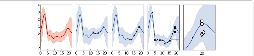
Gene expression experiments usually contain many types of effect aside from the one under study. In this case, the data includes cross-sectional effects which arise from array-specific and sample-specific causes, and are not due to the underlying time-series. These are treated as noise by our model, whereas PCA and KNN make no distinction between longitudinal and cross-sectional vari-ance and will freely impute these effects. This is illustrated in Figure 4, where cross-sectional effects mean that the missing datum’s true value lies below that seen by aver-aging the replicates, or imputed by HGP. The HGP and KNN methods, being sensitive to these effects impute the true value well, despite it being inconsistent across replicates.

To test the methods’ abilities to impute the replicable part of the signal, we tested the imputed values of the three methods against the median value for the missing time-point, averaged across replicates. We mea-sured the RMSE over the 100 imputations, and repeated the experiment 10 times with different randomisa-tions. The mean RMSE (over randomisations) and two standard deviations are shown in the first column of Table 2.

Another way to investigate the ability of the model to deal with missing data is to examine the differ-ence between the model as inferred with some missing points to that inferred with all the data: the results of doing so are shown in the second column of Table 2. Whilst this method may not give a completely fair reflection of the performance of the PCA and KNN methods, the small size of the errors on imputa-tion imply that our model is relatively insensitive to missing data: because the model can borrow statisti-cal strength from other replicates, small amounts of data missing at random make little difference to the model.

Figure 4An example of randomly missing data imputation.Here, the left-most pane shows the inferred mean function for the genegn(t), and

Table 2 RMSE of missing data imputation for hierarchical Gaussian processes (HGP) principal component analysis (PCA) and K-nearest neighbour (KNN)

Replicate median Full model

HGP 0.13±0.03 0.05±0.01

PCA 0.15±0.03 0.10±0.02

KNN 0.17±0.04 0.13±0.02

The first column shows the RMSE measured against the replicate-median, and the second column shows the RMSE against the model with no missing data.

Data fusion

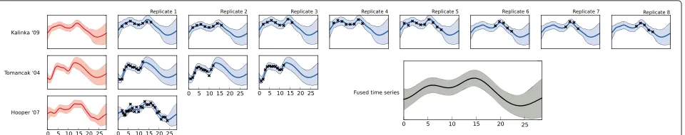
The data under investigation are sampled at two-hour intervals. To improve our knowledge of the system, it is possible to perform data fusion with existing data sets. We demonstrate this with two previous studies: [4,24], which offer more tightly temporally-spaced data, but with fewer replications (three and one respectively).

We constructed a hierarchical model across the three experiments, and across replicates within the experi-ments. The data were considered on a gene-by-gene basis, and the model was optimised for each gene. An example gene (Acer) is shown in Figure 5. The figure shows the inferred function for each replicate in each experiment, as well as the inferred mean function for each experiment (first column) and the inferred ‘top-level’ function (inset) which underlies all the experiments.

Clustering

In order to investigate the usefulness of our model in a clustering task, we first selected 300 dynamically differen-tially expressed genes using a method similar to [7].

We computed the marginal likelihood using our hierar-chical model and a simpler GP modelwithout replicate-specific or gene-replicate-specific variance. This model, simply fitting a GP to the lumped data is similar to the method proposed in [20], which represents the current state-of-the-art. Cookeet al[20] compared their method to sev-eral other algorithms and concluded that the GP method allowed for the discovery of clusters in a more effec-tive manner than non-temporal models. Here we show

that this method can be improved further by considering the gene-wise and replicate-wise intra-cluster structure of the data’s variance. For both models, we applied the EM algorithm with several restarts (varying the covari-ance function hyper-parameters on each restart), selecting the solution with the highest log-likelihood. We used our own implementation for Cooke et al.’s method to ensure that results were comparable: i.e. that improvements in the method were due to the HGP structure, rather than specifics of the implementation. We are primarily con-cerned with the improvements that the HGP model can offer in explaining cluster variance, and this allows for a direct comparison.

For further comparison, we used the R package Mclust [25]. Mclust fits a range of Gaussian models of increasing complexity; in the first instance, we simply concatenated the replicates and Mclust struggled to fit some models in the 56 dimensional space. Subsequently, we provided Mclust with shorter vectors formed by averaging the repli-cates at each time point, which gave similar results. We include the validation for both methods. In both cases, we used all available covariance structures for Mclust, and let the package pick the best using its BIC (Bayesian Information Criterion) approach.

In order to validate the different clusterings, we use the biological homogeneity index (BHI) [26], which assesses the number of genes with common function within each cluster, assigning the entire clustering a score from 0 to 1 with larger values corresponding to more biologically homogeneous clusters. For biological annotation, we used the three gene ontology (GO) categories (data obtained using biomaRt [27]), which correspond to molecular func-tion (MF), biological process (BP) and cellular component (CC). Computation of the BHI is then straightforward: it is the proportion of within-cluster pairs that share at least one biological annotation. The BHIs and log-likelihoods for all the experiments are shown in Table 3. We note that other comparisons between the clusters and the Gene Ontology may be possible, for example the GO term over-lap score [28,29], but we use the BHI here for ease of interpretability.

Table 3 Results of clustering 300 genes using the four proposed algorithms

MF BP CC L N. clust.

Agglomerative HGP 0.92 0.32 1.0 7360.8 50

agg. GP (as Cookeet al.) 0.78 0.26 0.72 6203.7 128

Mclust (concat.) 0.78 0.14 0.50 1324.0 26

Mclust (averaged) 0.80 0.16 0.42 -736.2 20

The first three columns report the Biological Homogeneity Index (BHI) for the gene ontology categories of Molecular Function (MF), Biological Process (BP) and Cellular component (CC). The two last columns report the log-likelihoodL of the models and the number of recovered clusters.

From the Table, it can be seen that HGP method improves the biological homogeneity for all three GO categories. By directly comparing with the standard GP method, we have demonstrated that the improvement in clustering performance is not due simply to the cluster-ing methodology or the GP correlations which give the GP method a small improvement over Mclust, but the hier-archical structure of intra-cluster variance which allows genes and replicates to differ in a temporally-correlated fashion.

Conclusions

We have presented a method based on hierarchically structured GPs, which are a practical and flexible frame-work for modelling replicated time-series. The frameframe-work has a wide range of applications, and can be extended for various data structures besides biological replications.

The method performed well in several tasks, including missing data imputation and clustering. We have shown that the method performs particularly well in missing data imputation, and that small amounts of missing randomly data have only a minor effect of the model. Biological validation through the BHI confirms the importance of modelling intra-cluster variance in a hierarchical fashion.

Above we showed how fitting the simplest of our pro-posed models can lead to a quantitative assessment of how biological replications are behaving, as well as illustrat-ing how our method deals with different types of replicate variation. Of course, if the replicate variance is truly inde-pendent – e.g. if only technical variation is present – then we recover standard GP regression. In this case the hierarchical approach requires the inclusion of an extra parameter, but we find that the additional computational complexity is negligible.

A problem with standard GP regression is that the com-putational complexity grows cubically with the number of data. We have presented a method which exploits the necessary condition that all genes in a cluster are mea-sured on the same time-points in order to significantly reduce the computational complexity and make our clus-tering algorithm applicable to large data sets. We note that

the complexity of the clustering algorithm scales poorly with the number of genes: the initial step of the algorithm must compare the likelihood of merging of each pair. To address this, randomised versions of the same algorithm can be adopted [30,31], and our hierarchical model and its efficient computation as (15) could be used with no modification.

Whilst we have demonstrated that our model is useful in several applications, we envisage a number of exten-sions. For example, our model could be used for data fusion of microarray data with high-throughput sequenc-ing data. Or, the hierarchical structure could be used in models of pathway activity [32], which may include prior information about gene groupings from Gene Ontology.

Although we have only used simple GP models within our hierarchical structure, the idea can be applied to more complex GP models, such as those proposed to model gene interactions [9,33].

Endnotes

a_{Other noise distributions are possible, but break the}

conjugacy of the model and thus complicate inference, see [10].

b_{Note that hierarchical in this sense means a}

hierarchical partitioning of the genes, distinct from our Bayesian hierarchical model applied within the cluster.

Appendix

Efficient computation of a cluster likelihood

The expression for the marginal likelihood of a cluster of genes as given in equation (15) can be derived by con-sidering the values of the underlying functionh(t)at the time pointst, which we denoteh. The model (for a single cluster) can be written:

p(Yi|Ti)=

p(h|t)

k∈ci

p(yk|h,t)dh. (16)

This consists of a prior for the latent variablehand a likelihood for the data associated with each gene in the cluster, conditioned on the latent variable. The objective here is to marginalise (integrate-out) the latent variable to achieve a tractable expression. Expanding equation (16),

p(Yi|Ti)=

(2π )−(N+1)D/2|n|−N/2|Kh|−1/2

exp ⎧ ⎨ ⎩−

1 2h

_K−1

h h

−1

2

k∈ci

(yˆk−h)n−1(yˆk−h)

⎫ ⎬ ⎭dh.

Some re-arrangement and completing the square inside the exponent leads to

p(Yi|Ti)=

(2π )−(N+1)D/2|n|−N/2|Kh|−1/2

exp ⎧ ⎨ ⎩−

1 2(h− ˆh)

_{(h− ˆh)}

−1

2hˆ

_hˆ−1 2

k∈ci ˆ

y_kn−1yˆk

⎫ ⎬ ⎭dh.

(18)

where we have defined for brevity=K−_h1+Ngn−1and ˆ

h=−1−1Ngy¯i. The first and third lines of this

expres-sion can be moved outside the integral, and we recog-nise the Gaussian nature ofexp

−1

2(h− ˆh)(h− ˆh)

dh = (2π )D/2||1/2_{. Substituting this and the}

expres-sions forhˆ andback into (18) leads to the expression given in (15).

Competing interests

The authors declare that they have no competing interests.

Authors’ contributions

JH designed the studies, implemented the algorithms in python and drafted the manuscript. MR and NDL assisted in design and analysis of the experiments. All authors read and approved the final manuscript.

Acknowledgements

This work was funded by EU FP7-KBBE Project Ref 289434, EraSysBio+ project SYNERGY (BBSRC award BB/I004769/2) and EU FP7 RADIANT (award no. 305626).

Author details

1_{Department of Computer Science, The University of Sheffield, Sheffield, UK.} 2_{Department of Neuroscience, The University of Sheffield, Sheffield, UK.} 3_{Faculty of Life Science, The University of Manchester, Manchester, UK.}

Received: 13 August 2012 Accepted: 13 August 2013 Published: 20 August 2013

References

1. Spellman P, Sherlock G, Zhang M, Iyer V, Anders K, Eisen M, Brown P, Botstein D, Futcher B:Comprehensive identification of cell cycle-regulated genes of the yeast Saccharomyces cerevisiae by microarray hybridization.Mol Biol Cell1998,9(12):3273.

2. Barenco M, Tomescu D, Brewer D, Callard R, Stark J, Hubank M:Ranked prediction of p53 targets using hidden variable dynamic modeling. Genome Biol2006,7(3):R25.

3. Straume M:DNA microarray time series analysis: automated statistical assessment of circadian rhythms in gene expression patterning.Methods Enzymol2004,383:149–166.

4. Tomancak P, Beaton A, Weiszmann R, Kwan E, Shu S, Lewis S, Richards S, Ashburner M, Hartenstein V, Celniker S, et al.:Systematic determination of patterns of gene expression during Drosophila embryogenesis. Genome Biol2002,3(12):0081–0088.

5. Sanguinetti G, Lawrence N, Rattray M:Probabilistic inference of transcription factor concentrations and gene-specific regulatory activities.Bioinformatics2006,22(22):2775.

6. Beal M, Falciani F, Ghahramani Z, Rangel C, Wild D:A Bayesian approach to reconstructing genetic regulatory networks with hidden factors. Bioinformatics2005,21(3):349.

7. Kalaitzis A, Lawrence N:A simple approach to ranking differentially expressed gene expression time courses through Gaussian process regression.BMC Bioinformatics2011,12:180.

8. Gao P, Honkela A, Rattray M, Lawrence N:Gaussian process modelling of latent chemical species: applications to inferring transcription factor activities.Bioinformatics2008,24(16):i70–i75.

9. Honkela A, Girardot C, Gustafson E, Liu Y, Furlong E, Lawrence N, Rattray M:Model-based method for transcription factor target identification with limited data.Proc Natl Acad Sci2010,107(17):7793. 10. Rasmussen C, Williams C:Gaussian Processes for Machine Learning.

Cambridge, Massachusetts and London, England: MIT press; 2006. 11. Ernst J, Nau G, Bar-Joseph Z:Clustering short time series gene

expression data.Bioinformatics2005,21(suppl 1):i159.

12. Gelman A, Carlin JB, Stern HS, Rubin DB:Bayesian Data Analysis. Boca Raton: CRC press; 2004.

13. Stegle O, Denby K, Cooke E, Wild D, Ghahramani Z, Borgwardt K:A robust Bayesian two-sample test for detecting intervals of differential gene expression in microarray time series.J Comput Biol2010,

17(3):355–367.

14. Liu Q, Lin K, Andersen B, Smyth P, Ihler A:Estimating replicate time shifts using Gaussian process regression.Bioinformatics2010,

26(6):770–776.

15. Ng S, McLachlan G, Wang K, Jones LBT, Ng SW:A mixture model with random-effects components for clustering correlated

gene-expression profiles.Bioinformatics2006,22(14):1745–1752. 16. Medvedovic M, Yeung K, Bumgarner R:Bayesian mixture model based

clustering of replicated microarray data.Bioinformatics2004,

20(8):1222.

17. Lin K, Chudova D, Hatfield G, Smyth P, Andersen B:Identification of hair cycle-associated genes from time-course gene expression profile data by using replicate variance.Proc Natl Acad Sci USA2004,

101(45):15955.

18. Dunson D:Nonparametric Bayes applications to biostatistics.In

Bayesian Nonparametrics. Edited by Hjort L, Holmes C, Muller P, Walker S. Cambridge: Cambridge University Press; 2010.

19. Heller K, Ghahramani Z:Bayesian hierarchical clustering.InProceedings of the 22nd International Conference on Machine Learning: ACM press; 2005:297–304.

20. Cooke E, Savage R, Kirk P, Darkins R, Wild D:Bayesian hierarchical clustering for microarray time series data with replicates and outlier measurements.BMC Bioinformatics2011,12:399.

21. Kalinka A, Varga K, Gerrard D, Preibisch S, Corcoran D, Jarrells J, Ohler U, Bergman C, Tomancak P:Gene expression divergence recapitulates the developmental hourglass model.Nature2010,468(7325):811–814. 22. Troyanskaya O, Cantor M, Sherlock G, Brown P, Hastie T, Tibshirani R,

Botstein D, Altman R:Missing value estimation methods for DNA microarrays.Bioinformatics2001,17(6):520.

23. Oba S, Sato M, Takemasa I, Monden M, Matsubara K, Ishii S:A Bayesian missing value estimation method for gene expression profile data. Bioinformatics2003,19(16):2088.

24. Hooper S, Boué S, Krause R, Jensen L, Mason C, Ghanim M, White K, Furlong E, Bork P:Identification of tightly regulated groups of genes during Drosophila melanogaster embryogenesis.Mol Syst Biol

2007,3:72.

25. Fraley C, Raftery AE:MCLUST: Software for model-based cluster analysis.J Classif1999,16(2):297–306.

26. Brock G, Pihur V, Datta S, Datta S:clValid: An R package for cluster validation.J Stat Softw2008,25(4):1–22.

27. Durinck S, Moreau Y, Kasprzyk A, Davis S, De Moor B, Brazma A, Huber W:

BioMart and Bioconductor: a powerful link between biological databases and microarray data analysis.Bioinformatics2005,

21(16):3439–3440.

28. Mistry M, Pavlidis P:Gene Ontology term overlap as a measure of gene functional similarity.BMC bioinformatics2008,9:327.

29. Kirk P, Griffin JE, Savage RS, Ghahramani Z, Wild DL:Bayesian correlated clustering to integrate multiple datasets.Bioinformatics2012,

30. Heller K, Ghahramani Z:Randomized algorithms for fast Bayesian hierarchical clustering.InPASCAL Statistics and Optimization of Clustering Workshop; 2005.

31. Darkins R, Cooke EJ, Ghahramani Z, Kirk PD, Wild DL, Savage RS:

Accelerating Bayesian hierarchical clustering of time series data with a randomised algorithm.PloS one2013,8(4):e59795.

32. Shi Y, Klustein M, Simon I, Mitchell T, Bar-Joseph Z:Continuous hidden process model for time series expression experiments.Bioinformatics

2007,23(13):i459–i467.

33. Lawrence N, Girolami M, Sanguinetti G, Rattray M:Learning and Inference in Computational Systems Biology. Cambridge: MIT press; 2010.

doi:10.1186/1471-2105-14-252

Cite this article as:Hensmanet al.:Hierarchical Bayesian modelling of gene expression time series across irregularly sampled replicates and clusters. BMC Bioinformatics201314:252.

Submit your next manuscript to BioMed Central and take full advantage of:

• Convenient online submission

• Thorough peer review

• No space constraints or color figure charges

• Immediate publication on acceptance

• Inclusion in PubMed, CAS, Scopus and Google Scholar

• Research which is freely available for redistribution