Blind channel estimation using redundant precoding : new algorithms, analysis, and theory

(1)

Algorithms, Analysis, and Theory

Thesis by

Borching Su

In Partial Fulfillment of the Requirements for the Degree of

Doctor of Philosophy

California Institute of Technology Pasadena, California

2008

(2)

c

2008

(3)

Acknowledgments

I would like to first express my sincerest gratitude to my thesis advisor, Professor P. P. Vaidyanathan, for his excellent guidance, encouragement, and patience during the years of my Ph.D. study at Cal-tech. P. P. not only has taught me valuable skills for doing research, but has also influenced me with invaluable attitudes required for a real scholar. His advices have been inspiring and motivat-ing, and his words of encouragement have always been a strong support especially when I faced difficulties. He made me understand the importance of being confident yet polite, assertive yet consistent, and disciplined yet humorous. And the fact that he lives with these values himself un-compromisingly is a stronger source, than words, of stimulation and reinforcement for my research endeavors. He is in every aspect a great teacher and advisor, and I feel really grateful and fortunate to be one of his students.

I would also like to thank the members of my defense and candidacy examining committees for their interest: Professor Robert McEliece, Professor Babak Hassibi, Professor Yaser Abu-Mostafa, Professor Tracey Ho, and Dr. Andre Tkacenko. Generous support from Moore Fellowship, National Science Foundation, and the Office of Naval Research is gratefully acknowledged. I would also like to thank DSP lab alumni and frequent visitors Professor See-May Phoong and Professor Yuan-Pei Lin, whose comments have in my early years helped me find my initial research direction.

I would like to thank my labmates, Andre Tkacenko, Michael Larsen, Sriram Murali, Byung-Jun Yoon, Chun-Yang Chen, and Ching-Chih Weng, for their friendship and sharing experience in learning and research during my stay in the DSP lab. I would especially like to thank Byung-Jun, with whom I shared the longest time in the lab, for his constant thoughtful support since my first day in the lab. I would also like to Chun-Yang and Ching-Chih for all the stimulating discussions and memorable joyful moments we have shared in the lab.

(4)

(5)

Abstract

Digital signal processing (DSP) techniques have played an important role in channel equalization and estimation in communication systems. While channel equalization and estimation are usually done by pilot-assisted methods in most systems, algorithms for blind channel estimation have also been largely studied due to high bandwidth efficiency. However, up to date, most blind methods possess disadvantages such as slow convergence speed, high complexity, poor performance, etc., compared to pilot-assisted methods. These drawbacks have made many consider blind methods as inapplicable in modern communication systems which feature fast-varying channels.

In this thesis, we consider the blind channel estimation problem in block transmission systems with linear redundant precoding (LRP) which have been widely adopted in modern communica-tion systems in recent years. The main contribucommunica-tion of this thesis is to considerably reduce the amount of received data required for blind estimation and suggest blind methods which are appli-cable even in fast-varying environments (e.g., in wireless channels). New algorithms are proposed, performance analysis derived, and theoretical issues studied.

The first part of the thesis focuses on new algorithms for blind channel estimation and blind block synchronization in LRP systems. Two major types of linear redundant precoding, namely zero-padding (ZP) and cyclic prefixing (CP), are considered in this thesis. We first propose a gen-eralized, subspace-based algorithm for blind channel estimation in ZP systems of which two pre-viously reported algorithms are special cases. The generalization uses an integer parameter called

repetition indexwhich represents the number of repeated uses of each received block. The number of received blocks required for subspace-based blind estimation is roughly inversely proportional to the repetition index. By choosing a larger repetition index, the amount of received data can be significantly reduced.

(6)

orthog-onal frequency division multiplexing (OFDM) systems. The use of repetition index in CP systems is much less obvious and conceptually more complicated than in ZP systems. By choosing a repe-tition index larger than unity, the number of received blocks needed for blind estimation is signifi-cantly reduced compared to all previously reported methods. Theoretically, the proposed method can perform blind estimation using only three received blocks in absence of noise. In practice, the number of received blocks needed to yield a satisfactory bit error rate performance is usually on the order of half the block size. The proposed algorithm can be directly applied in OFDM systems without any modification of transmitter structure. A semiblind algorithm for channel estimation in OFDM systems is also proposed based on the extension of the blind algorithm.

Another important problem, namely the blind block synchronization, is also studied. Most existing blind estimation methods in LRP systems assume the block boundaries of the received streams are perfectly known to the receiver, but this assumption is usually not true in practice since no extra known samples are transmitted. Two algorithms for blind block synchronization are pro-posed for ZP and CP systems, respectively. In particular, the block synchronization problem in CP systems is a broader version of the timing synchronization problem in the OFDM systems. The proposed algorithms exploit the concept of repetition index and both theoretical and simulation re-sults suggest their advantages over all previously reported algorithms, especially when the amount of received data is limited.

(7)

List of Figures

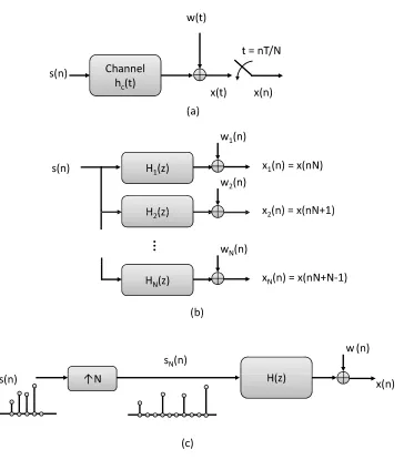
1.1 Baseband representation of a digital communication channel. (a) Analog model with a bandlimited channel impulse responsehc(t); (b) Equivalent digital model with

chan-nel transfer functionH(z). . . 3

1.2 Single-input-multiple-output channel model. (a) Oversampling of a SISO channel; (b) A SIMO channel; (c) Equivalent system with an upsampled source signal. . . 5

1.3 Schematic of subspace based system identification. . . 6

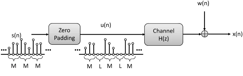
1.4 Illustration of a zero-padding precoder and a cyclic-prefixing precoder. . . 7

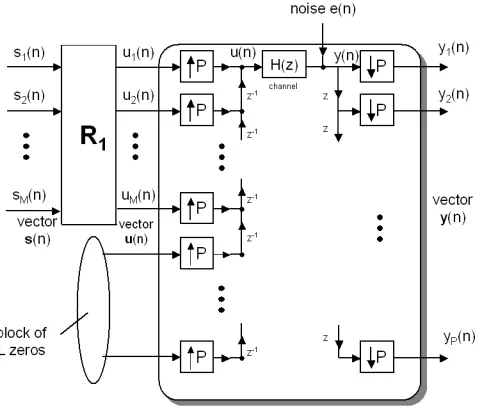
1.5 A block transmission system with a linear redundant precoderR(z). . . 8

2.1 Communication System with Redundant Filter Bank Precoders. . . 17

2.2 The zero-padding system with precoderR1. . . 18

2.3 Q-repetition and shifting operation. . . 24

2.4 Receiver structure for frequency domain approach. . . 26

2.5 Normalized least squared channel error estimation. . . 32

2.6 Bit error rate performance of the blind algorithm. . . 33

2.7 Normalized least squared channel error estimation. . . 34

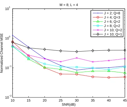
2.8 Normalized Channel MSE performance for a time-varying channel. . . 37

2.9 Bit error rate performance for a time-varying channel. . . 37

3.1 A typical cyclic prefix system. . . 44

3.2 The transceiver system equipped with a method to resolve scale-factor ambiguity. . . 61

3.3 A CP-based orthogonal frequency division multiplexing (OFDM) system. . . 63

3.4 Illustration of the approach of the proposed semi-blind estimation algorithm. . . 64

3.5 The probability ofU(_QJ)having full rank in SC-CP systems. . . 67

(14)

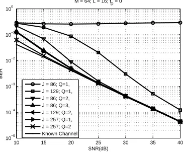
3.7 Normalized mean squared error of channel estimation for static channels with the QPSK constellation in SC-CP systems. . . 71 3.8 Bit error rate performance for static channels with the QPSK constellation in SC-CP

systems. . . 71 3.9 Bit error rate performance for static channels with the 16-QAM constellation in SC-CP

systems. . . 71 3.10 Bit error rate performance for static channels with the QPSK constellation in OFDM

systems. . . 72 3.11 Bit error rate performance for static channels with the QPSK constellation in SC-CP

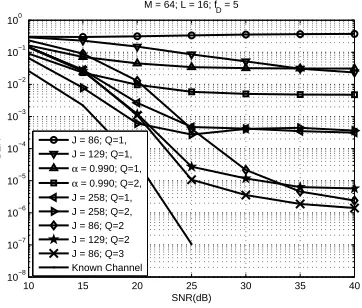
systems whenJis small. . . 73 3.12 Bit error rate performance for blind estimation systems when the Doppler frequency

is 5 Hz (5.4 km/hr). . . 73 3.13 Bit error rate performance for blind estimation systems when the Doppler frequency

is 50 Hz (54 km/hr). . . 73 3.14 Pilot positions forK= 20(left) andK= 15(right). . . 76 3.15 Comparison of pilot-based and semi-blind methods in channel estimation mean square

error performance. . . 77 3.16 Comparison of pilot-based and semi-blind methods in bit error rate performance. . . 78

4.1 Block transmission systems using linear redundant precoders. . . 85 4.2 Illustration of blind block synchronization problem in ZP and CP systems. . . 85 4.3 Functionλ(d)v.s. time mismatchdfor a channel with zeros at(0.8,−0.8,0.5j,−0.5j)

in absence of noise. . . 100

4.4 Blind block synchronization error rate performance for a channel with zeros at(0.8,−0.8,0.5j,−0.5j) whenJ= 20in ZP systems. . . 100

4.5 Functionλ(d)v.s. time mismatchdfor a channel with zeros at(1.2,−0.9,0.7j,−0.7j) in absence of noise whenJ = 20. . . 101

4.6 Blind block synchronization error rate performance for a channel with zeros at(1.2,−0.9,0.7j,−0.7j) whenJ= 20in ZP systems. . . 101

(15)

4.8 Blind block synchronization error rate performance for a Rayleigh random channel with smallJ in ZP systems. . . 102 4.9 Blind block synchronization error rate performance for a channel with zeros at(0.8,−0.8,0.5j)

whenJ= 40in CP systems. . . 104 4.10 Blind block synchronization error rate performance for a channel with zeros at(1.2,−0.9,0.7j)

whenJ= 40in CP systems. . . 105 4.11 Blind block synchronization error rate performance for a third-order Rayleigh random

channel withJ = 40in CP systems. . . 105 4.12 Blind block synchronization error rate performance for a fourth-order Rayleigh

ran-dom channel withJ= 40in CP systems. . . 106 4.13 Blind block synchronization error rate performance for a third-order Rayleigh random

channel in CP systems whenJ is small. . . 106

5.1 Channel estimation MSE versus SNR obtained by simulations, theoretical values in (5.7), and CRB in (5.11) with 16 blocks. . . 123 5.2 Channel estimation MSE versus SNR obtained by simulations, theoretical values in

(5.7), and CRB in (5.11) with 5 blocks. . . 124

7.1 A multi-input multi-output LTI system. . . 163 7.2 Distribution of degree of non-richness of signals whose entries are from BPSK

constel-lation. . . 180 7.3 Distribution of degree of non-richness of signals whose entries are from QPSK

con-stellation. . . 181 7.4 Distribution of degree of non-richness of signals whose entries are from 16-QAM

(16)

List of Tables

2.1 Coefficients for the Time-Varying Channel. . . 36

3.1 Power delay profile of the channel model used in Section 3.6 . . . 69

5.1 Comparison of Eq. (33) in [2] and Eq. (5.11); the data length per block isM = 12 . . . 125

(17)

Chapter 1

Introduction

In digital communication systems, channel equalization and channel estimation are essential to successful data transmission. While channel equalization and estimation are usually done by pilot-assisted-based methods (i.e., inserting pilot samples that are known to the receiver into the trans-mitted data sequence), blindmethods have also been developed (see [8] and references therein) which do not require use of pilot samples and possess desirable advantages such as a better band-width efficiency. Although many blind methods in various types of communication systems have been developed since the early 80s, they generally suffer from several drawbacks which prevent them from widespread use.

As block transmission systems using redundant precoding, such as orthogonal frequency di-vision multiplexing (OFDM) systems, become increasingly popular, research on blind channel es-timation has also been shifted to these types of systems. Recent work on block transmission sys-tems with redundant precoding [45] has shown that the redundancy, originally introduced for the purpose of eliminating interblock interference (IBI), is also beneficial to blind channel estimation. Many blind methods have been developed for block transmission with different types of redundant precoding and prove to be free from several problems present in conventional blind channel esti-mation [30]. These new algorithms, however, still have several problems such as slow convergence speed (i.e., requirement of a large amount of received data), which makes them less applicable in an environment where the channel status is fast-varying (e.g., in a wireless link). Other problems include computational complexity, constraints on data constellations, etc.

(18)

estimation, and the signal richness preservation problem, will also be considered in this thesis. In this introductory chapter, we give an overview of the basic concepts and a brief history of blind channel estimation. Every attempt is made to make the present text as self-contained as possible, and the introduction is meant to primarily serve this purpose. Due to the large volume of the blind channel estimation literature, the summary here is only directly related to the thesis topics and is by no means a complete treatment of all past work. The readers interested in more comprehensive treatments are referred to [8, 11].

1.1

Brief History of Blind Channel Estimation

Figure 1.1 depicts the baseband representation of a digital communication system. The communi-cation channel is characterized as a linear time invariant (LTI) system which has a finite impulse response (FIR) due to finite delay spread of the channel. The impulse responsehc(t)is a cascade of

the pulse shaping filter in the transmitter, the physical multipath fading channel, and the receive filter. Assume the symbol interval of the input signal isT. The output signal can be written as

x(t) =X

n

s(n)hc(t−nT) +w(t).

When the output signal is sampled at the baud rate (i.e., at the rate1/T), the system can be simplified as in Figure 1.1-(b), where the equivalent channel,H(z), is a discrete LTI system. The received signalx(n)is a noise corrupted version of the convolution of the input signals(n)and the channel impulse responsehc(t). A successful communication aims at recovering the

(19)

w (t )

s (n ) C h a

n n e l

h c

(t )

t

=

n T

(

a

)

c

( ) x

(n )

x

(t )

w (n )

s (n ) C h a

n n e l

H

(z ) x

(n )

[image:19.612.215.430.57.284.2]

(b )

Figure 1.1: Baseband representation of a digital communication channel. (a) Analog model with a bandlimited channel impulse responsehc(t); (b) Equivalent digital model with channel transfer

functionH(z).

1.1.1

Early Developments of Blind Estimation in SISO Systems

Since the late 70s, many blind equalization algorithms have been proposed [40, 12, 3, 47]. Most of these early developments of blind methods are based on adaptive algorithms. They generally share the following features. First of all, although the explicit knowledge ofs(n)is unknown, the constel-lation used bys(n)must be known and is usually quadrature amplitude modulation (QAM), pulse amplitude modulation (PAM), or phase shift keying (PSK). A special class of these algorithms is the constant modulus algorithm (CMA) [12], which works by setting constant modulus constraints on samples equalized by adaptive filters. Also, higher-than-second-order-statistics (HOS) of the received stream is required in these algorithms. The requirement for HOS may be explained as follows. Evaluating the spectral density function of the output signal, we have

Sxx(z) =|H(z)|2Sss(z) +Sww(z),

whereSxx(z) , PmE[x(n)x∗(n−m)]z−m, Sss(z) , PmE[s(n)s∗(n−m)]z−m, andSww(z) , P

mE[x(n)x∗(n−m)]z−m. Assume the input spectral density functionSss(z)is known (usually

(20)

H(z)is missing. In order to obtain the full information of the channel, higher-than-second-order statistics (HOS) ofx(n)is employed in many blind algorithms (e.g., 4th order) [47].

These early algorithms in general share the following common drawbacks. First of all, the con-vergence of the adaptive algorithms depends on the initial values of the equalizer parameters, and the solution is subject to local convergence. Secondly, due to the use of HOS, the required amount of received data is usually very large, and this makes the algorithms have slow convergence time and inapplicable in time-varying environments. Finally, the computational complexity is high for HOS of received data. These drawbacks limit their applicability in practical situations.

1.1.2

Using Second Order Statistics in SIMO Systems

It is shown above that second order statistics (SOS) of received samples alone cannot give the full information of a frequency selective channel. However, since algorithms based on second order statistics converge much faster than those using higher-order statistics, researchers have searched for newer methods. The work proposed by Tonget al. in 1991 which first used only SOS of the re-ceived samples for blind channel estimation in the context of single-input-multiple-output (SIMO) systems is widely considered as a major breakthrough. As shown in Figure 1.2, a set of virtual mul-tiple channels can be achieved by oversampling at the receiver in a physically SISO system. The work in [64] suggests SOS alone is sufficient to estimate channel coefficients blindly as long as the oversampled channel satisfies a channel diversity condition. Following this, considerable research has been done to study blind channel estimation in SIMO systems using SOS [26, 27, 30, 46, 74]. Among these, a representative is a subspace based algorithm proposed by Moulineset al. in [30], which explicitly exploits the signal and noise subspace separation and also the special structure of the channel matrix. First used in the famous multiple signal classification (MUSIC) algorithm [42], the basic idea of subspace-based methods are illustrated in Figure 1.3 and are elaborated below.

The first principle of subspace-based algorithms is that the dimension of the observation space, q, must be strictly larger than that of the signal space,p. The matrixH_θhas a known structure in terms of an unknown parameter vectorθ_{. By evaluating the autocorrelation matrix of} _y(n)_and

an eigen-decomposition ofRyy, the basis vectors of signal space and noise space can be found. Finally, using the fact that the noise space is orthogonal to the space spanned by all columns of the matrixH_θ, the parameter vectorθ_{can be found. In the case of blind estimation in SIMO channels,}

(21)

w (t )

t

=

n T / N

(a )

s (

n

) C h

a

n n e l

h c

(t ) x

(

n

)

x

(t )

(a )

( ) (

N

)

w 1 (

n

)

s (

n

) H 1 (z )

H (z )

x 1 ( n )

=

x ( n N ) x 2 ( n ) = x (

n N + 1

) w 2 ( n ) H 2

(z )

x 2 ( n ) x (

n N + 1

)

w N (

n

)

H N (z )

x N ( n )

=

x (

n N + N

Ͳ

1

)

(b )

( )

s N

(n ) w

(n )

s

(n ) H

(z ) x

(n )

ј

N [image:21.612.148.512.130.545.2]

(c )

(22)

w (n )

T

y

(n )

( )

p q

>

s (n )

C a lc u lat e

A u t o

Ͳ

c o rre lat io n

m

at rix

K n o w le d g e

o f

s

t ru ct u re

o f

H T

y

(n )

q > p

b

R y y

T

^

†

N oise

space

d im :(q

Ͳp)

S u b s p a c e

d e c o m p o s it io n

R y y =

H T

R

s s

H T

† +

R

w w S ig na l

s p

ace

d

im :

p

Figure 1.3: Schematic of subspace based system identification.

the matrixH_θ has a special block Toeplitz structure [30]. Subspace-based algorithms have since played an important role and are still widely used in the development of blind channel estimation algorithms nowadays.

There are two problems with blind methods in SIMO systems which prevent them from practi-cal applications. First of all, most of these methods are very sensitive to channel order overestima-tion: they require the maximum channel order among the multiple channels to be exactly known. This information, however, is usually unavailable in most situations. The second problem is the bandwidth expansion caused by oversampling at the receiver. As illustrated in Figure 1.2-(c), the SIMO channel is equivalent to a SISO channel where the source signal is upsampled by a factor of N[9].

1.2

Blind Channel Estimation Using Redundant Precoding

(23)

w (n )

C h a

n n e l

( )

Z

e ro

u

(n )

s (n )

C h a

n n e l

H

(z ) x

(n )

P a d d i

n g

M M M

M L

[image:23.612.117.523.57.185.2]

M L M

Figure 1.4: Illustration of a zero-padding precoder and a cyclic-prefixing precoder.

(asymptotically unity) and is robust to channel order overestimation. So blind methods developed in LRP systems are in general superior to those in SIMO systems. In this section, we will first review block transmission systems with linear redundant precoders and then review blind channel estimation algorithms with redundant precoding.

1.2.1

Block Transmission Systems With Linear Redundant Precoders

To illustrate the idea of linear redundant precoding, we first explain a special case called “zero-padding.” As shown in Figure 1.4, the source sequences(n)is divided into blocks of sizeM. A zero block of lengthLis inserted after each block. SupposeP =M+L. Then mathematically,

u(nP+k) =

  

s(nM+k) if0≤k≤M−1 0 ifM ≤k≤P−1 .

The zero-padding precoder introduces bandwidth expansion by a factor(M +L)/M. While the redundancy lengthLis usually chosen as an integer comparable to the channel order, the block sizeM can be chosen as any positive integer. WhenM is chosen as a large integer, the bandwidth expansion factor is asymptotically unity. The general form of a block transmission system with linear redundant precoder is shown in Figure 1.5. The source sequences(n)is blocked into vectors s(n)of sizeM:

s(n) =h s(nM) s(nM + 1) · · · s(nM+M−1)

iT

.

The vectorss(n) go through a linear precoder characterized as a P ×M polynomial matrix in z−1_,_{R(z) =}PK

k=0Rkz−k, resulting in aP-vectoru(n) =

PK

(24)

b l k i i t l i b l k i

e (n )

y

(n )

( ) u

(n )

s (n ) u (n )

b lo c k in g in te rle a v in g

p

n

p

y

(n )

b lo c k in g

s (n )

z z Ͳ

1

p

M

p

M

n

P

n

P

H

(z )

p

P

p

P

z R

(z )

z Ͳ

1

z

p

z Ͳ

1

p

M

n

P

p

P

n

P

p

P

Figure 1.5: A block transmission system with a linear redundant precoderR(z).

interleaved into the precoded sequenceu(n)which is sent over the channelH(z).

The zero-padding precoder illustrated in Figure 1.4 is a special case whereR(z)is chosen as

R(z) =



 IM

0

 ,

whereIM is theM×M identity matrix. A more general zero-padding precoder has transfer

func-tion of the form

R(z) =

  R1(z)

0

 ,

whereR1(z)is anM×M polynomial matrix inz−1_.

Another important class of linear redundant precoders is cyclic prefix (CP) precoders. A CP precoder has a transfer function

R(z) =



 Rcp(z)

R2(z)

 ,

whereR2(z)is anM×Mpolynomial matrix inz−1_and_R

cp(z)is anL×Mmatrix whose elements

(25)

The linear redundant precoders were proposed in an attempt to eliminate interblock interfer-ence (IBI) of the received blocks caused by the frequency selective channelH(z)[73]. If the channel order ofH(z)is upper-bounded byL, the received blocks will be free of interblock interference and channel equalization can be performed block-by-block without worries of interblock error propa-gation. Noise amplification can be avoided in the channel equalization phase even if the channel has zeros outside the unit circle. It turns out the redundancy introduced by LRPs are also helpful in blind channel estimation, as discussed below.

1.2.2

Blind Channel Estimation in LRP Systems: Subspace v.s. Finite Alphabet

Algorithms

The blind channel estimation algorithms in LRP systems can be roughly divided into two cate-gories: finite-alphabet-based algorithms and non-finite-alphabet algorithms. Algorithms that ex-ploit knowledge of the finite-alphabet of the source data generally have a shorter converge time but may be computationally exhausting when the constellation size is large [76, 6]. Most non-finite-alphabet-based algorithms exploit (second order) statistics of the received data [15, 35]. These methods naturally require a longer convergence time than finite alphabet counterparts before an accurate channel estimate can be obtained due to use of statistics. Another important category of non-finite-alphabet-based algorithms uses subspace decomposition [5, 21, 45], and they can even be implemented deterministically [45, 36, 5, 21, 32].

Subspace-based algorithms can be used in any kind of constellation, but require a longer con-vergence time. We will discuss subspace based channel estimation algorithms for ZP systems and CP systems here. In ZP systems, the first subspace-based blind channel estimation algorithm was proposed by Scaglioneet al. [45]. Subspace algorithms in CP systems require more sophisticated designs [5, 21, 32]. These methods all need the persistency of excitation property of the input sig-nal (i.e., sigsig-nal richness) to render the data covariance matrix to have full rank. This requirement demands the receiver to collect at least a number of blocks equal to the block size for one channel estimate and thus makes the approach less applicable when the channel is fast-varying.

(26)

out by Mantonet al. [28] that a blind estimation without knowledge of finite alphabet in ZP sys-tems is possible with onlytworeceived blocks. An algorithm based on viewing the channel estima-tion problem as finding the greatest common divisors (GCD) of polynomials representing received blocks was proposed in [36].

Although many blind algorithms in LRP systems have been developed, they mostly tend to suffer from several common drawbacks such as slow convergence speed, high complexity, poorer performance, etc., as opposed to pilot-assisted methods. In this thesis, we propose new algorithms and theories that suggest blind algorithms can in general be developed with small amount of re-ceived data, satisfactory system performance, and reasonable complexity.

1.3

Outline of the thesis

1.3.1

Scope of the thesis

There are two major parts in this thesis. In the first part (Chapters 2, 3, and 4), new algorithms for blind channel estimation using redundant precoding as well as other related problems, including blind block synchronization and semi-blind channel estimation, are proposed. The second part of the thesis (Chapters 5, 6, and 7) deals with theoretical aspects of the blind channel estimation prob-lems, including performance analysis of the blind algorithms, and the signal richness preservation problem. In this section we will briefly introduce the scope of each chapter.

1.3.2

Generalized Algorithms for Blind Channel Estimation in ZP Systems

(Chap-ter 2)

The material in Chapters 2 and 3 presents new algorithms for blind channel estimation in LRP systems. Chapter 2 studies the blind channel estimation algorithm in ZP systems, i.e., the precoder R(z)has a form ofR(z) =h R1(z)T ₀T iT_{. The proposed algorithm is a generalization of two}

(27)

common divisor (GCD) of polynomials representing received blocks. The MNP algorithm requires only two blocks to work but has much more computational complexity.

Although the MNP method is based on the idea of the greatest common divisor of polynomials, the mathematical formulation of its implementation still involves subspace decomposition (in a space of a larger dimension). This fact puts the MNP method and the SGB method into the same category, and we can generalize them using a concept called repetition index. In Chapter 2, we will propose a generalized algorithm of which the SGB algorithm proposed in [45] and the MNP algorithm in [36] are both special cases. The idea of repetition index is to repeatedly use each received block. In the conventional subspace method, the receiver needs to accumulateM blocks in order to achieve sufficient rank. By repeated use of each received block by a factor ofQ, the number of blocks needed to achieve the required rank can be significantly reduced and is roughly inversely proportional to the repetition indexQ. The MNP method essentially uses a large repetition index (Q = P) and requires only two received blocks. The use of a largeQalso increases the receiver side computational complexity. By carefully choosing parameters, the system performance and computational complexity can be jointly optimized.

1.3.3

Blind and Semi-Blind Channel Estimation in Cyclic Prefix Systems

(Chap-ter 3)

(28)

the proposed method to perform blind identification using only three received blocks in absence of noise. We also study a semi-blind channel estimation algorithm in OFDM systems which is a special case of CP systems. The proposed semi-blind estimation algorithm is a combination of the blind channel estimation method and a pure pilot-assisted method. Simulation results show that, under the same number of pilot samples, the semi-blind algorithm has a clear improvement over the pure pilot-assisted method.

1.3.4

New Algorithms for Blind Block Synchronization In LRP Systems

(Chap-ter 4)

Many algorithms for blind channel estimation in LRP systems, including those proposed in Chap-ters 2 and 3, are based on the assumption that block synchronization is perfect, i.e., block bound-aries of the received streams are perfectly known to the receiver. In practical applications, however, this assumption is usually not true since no extra known samples are transmitted. The problem of blind block synchronization is therefore important. However, up to date, this problem has not yet been given as much attention as blind channel estimation has. Chapter 4 studies the blind block synchronization problem in both ZP and CP systems. These algorithms exploit the presence of rank deficiency in the matrix composed of received blocks when the block synchronization is perfect. The formulated matrices, when block synchronization is not correct, have a higher rank instead. In order to make the matrices have sufficiently large rank, a large amount of received data is required for both algorithms. The algorithms proposed in Chapter 4 use the concept of repetition index and guarantee correct block synchronization in absence of noise using only two and three received blocks in ZP and CP systems, respectively, when the repetition index is chosen appropriately.

1.3.5

Performance Analysis of Blind Estimation Algorithms in ZP Systems

(Chap-ter 5)

(29)

the-oretically. We study the channel estimation error (MSE) in the algorithm of [49] and compare it with the corresponding Cramer-Rao bound. We will derive in this chapter performance analysis of the generalized algorithm proposed in Chapter 2. When the number of received blocks is small, however, there is an obvious gap between the performance of the SGB algorithm and the corrected CRB given in [58] when a small number of received blocks are available. Both theory and simula-tion results suggest that the performance of the generalized algorithm is usually closer to the CRB when the repetition index is larger but the performance does not achieve the CRB for any repetition index.

1.3.6

Theoretical Issues on Signal Richness Preservation for Blind Estimation

(Chapters 6 and 7)

In Chapters 6 and 7, we study in detail theoretical issues on signal richness in ZP systems, specifi-cally the richness preservation problem. The richness property of input signals is essential to blind channel estimation algorithms we discussed in Chapter 2. Since the property of signal richness may be altered by a linear precoder, we are interested in finding the conditions on which a this lin-ear precoder will “preserve” the property of signal richness. For different blind channel estimation algorithms, the definition of signal richness may be different. Conventionally, signal richness can be defined as follows. A signal ofM-vectorsx(n), n≥0, is said to berichorrank richif the matrix

h

x(0) x(1) · · · x(Kx) i

has rankM for sufficiently largeKx. This definition of signal richness is required for input signals

used in the SGB method [45] (see Sec. 1.3.2). We say a ZP precoderR(z)is richness-preserving if for any rich input signalx(n), the output ofR(z)is also rich. The mathematical problem on richness-preserving precoders, rather than the application itself, is the focus of Chapter 6. It turns out that there exist only two major types of systems which preserve richness.

(30)

finding the solution of the problem, a new class of invertible matrices, namely the Vandermonde-form preserving (VFP) matrices, is introduced. Several interesting properties of the VFP matrices are also studied.

1.4

Notations

The notations used throughout this thesis are defined as follows. Boldfaced lower case letters rep-resent column vectors. Boldfaced upper case letters and calligraphic upper case letters are reserved for matrices. Superscripts∗,T, and † as ina∗_,_AT_{, and}_A† _{denote the conjugate, transpose, and}

transpose-conjugate operations, respectively. A#represents the pseudo-inverse ofA. H(z)e repre-sentsH†(1/z∗_)._[v]

idenotes theith element of vectorv,[A]idenotes theith row of matrixA, and

[A]_ij denotes the entry at theith row and thejth column of matrixA. Column and row indices of all vectors and matrices begin at one. ei,M denotes the ith column of the identity matrixIM

and is often abbreviated asei when there is no ambiguity about the value ofM. All the vectors

and matrices in this paper are complex-valued. The notationWM denotese−j2π/M, andWM is the

M×Mnormalized DFT matrix whosekl-th entry isW_M(k−1)(l−1)/√M. Column and row indices of all matrices and vectors begin at one.Ak,lis the entry at thekth row and thelth column ofA.Inis

then×nidentity matrix, and0m×nis them×nzero matrix. In figures, “↑N” and “↓N” denote the

signal downsampler and upsampler, respectively [67]. The notation vec(A)represents the column vector constructed by concatenating columns ofA. A_⊗Bdenotes the Kronecker product[17] of the matricesAandB.

A matrixTis said to be aToeplitz matrixifThas constant values along diagonals, i.e.,[T]ij =

[T]i+k,j+k for alli, j, k such that the indices ofTin the above equation are within the size ofT.

A matrix His said to be aHankel matrix ifH has constant values along all skew diagonals, i.e., [H]ij = [H]i+k,j−k for alli, j, k such that the indices of Hin the above equation are within the

size of H. Notations for commonly used matrix structures in this paper are presented below. If v = h v1 v2 · · · vm

iT

(31)

full-banded Toeplitz matrix

Tn(v) =                  

v1 0 · · · 0

v2 v1 . .. ... ..

. v2 . .. 0 vm ... . .. v1

0 vm v2

..

. . .. ... ... 0 · · · 0 vm

                  (1.1)

andKl(v)to denote thel×(m−l+ 1)Hankel matrix

Kl(v) =         

v1 v2 v3 · · · vm−l+1

v2 v3 . .. . .. ... ..

. . .. . .. . .. vm−1 vl · · · vm−1 vm

         . (1.2)

Due to the special property of cyclic prefixes, we will use the following notation extensively in this paper. Supposeyis anm×1column vectory=h y1 y2· · · ym

iT

. Then, the notation[y]_a_:_b denotes the(b−a+ 1)×1vector

[y]_a_:_b =h ya ya+1 · · · yb iT

if1≤a≤b≤m. An extension of this definition to any arbitrary pair of integersaandbsatisfying a ≤ b is made by defining yk asy₍_k₋₁_mod_m₎₊₁ for anyk > mork < 1. For example, ify = h

y1 y2 y3

iT

, then[y]₋_1:7denotes the vectorh y2 y3 y1 y2 y3 y1 y2 y3 y1

iT

(32)

Chapter 2

Generalized Algorithms for Blind

Channel Estimation in Zero-Padding

Systems

In this chapter, we study the problem of blind channel estimation in zero-padding (ZP) systems. As shown in Chapter 1, redundancy introduced at the transmitter facilitates blind identifiability of channel coefficients using only second order statistics (SOS) of received samples. The problem of blind channel estimation in ZP systems was first studied in [45]. By exploiting the padded zeros between data blocks, Scaglioneet al. proposed a subspace based method, which we will call the SGB method. The SGB method not only works with SOS of received samples, but can also be implemented using deterministic received data, as long as the source signal is rich or rank rich. That is, the matrix composed of finite source blocks achieves full rank. The SGB method is robust to channel order overestimation. Furthermore, the bandwidth expansion factor is asymptotically unity when the block size goes to infinity. These two advantages make the SGB method superior to other blind channel estimation algorithms in virtual SIMO systems.

(33)

Figure 2.1: Communication System with Redundant Filter Bank Precoders.

the GCD idea is also based on subspace decomposition [39]. This similarity of the two algorithms suggests a possibility of generalization.

In this chapter, we propose such a generalized, subspace-based algorithm of which both the SGB method [45] and the MNP method [36] are special cases. The generalization uses an integer parameter calledrepetition index which represents the number of repeated uses of each received block. The choice of the repetition index is roughly inversely proportional to the number of re-quired received blocks. When the repetition index is chosen as unity, the algorithm reduces to the SGB method; when it is equal to the size of a received block, it becomes the MNP algorithm. The large repetition index of the MNP method explains its speedy convergence and suitability in fast-varying environments but also imposes a high computational complexity. The introduction of repetition index provides a way to achieve a system performance similar to or better than that of the MNP method with a much less computational load.

The content of this chapter is mainly drawn from [49], and portions of it have been presented in [51]. Other relevant results will be presented in later chapters. The performance analysis of the generalized algorithm will be presented in Chapter 5. Some theoretical issues on signal richness will be studied in Chapters 6 and 7.

2.1

Outline

(34)

[image:34.612.206.448.51.255.2]

Figure 2.2: The zero-padding system with precoderR1.

sequence under which the algorithm operates properly. In Section 2.4 a variation of the generalized algorithm, namely the frequency domain version of the generalized algorithm, is proposed.

The conditions on the input signal under which the proposed algorithms work properly result in the concept ofgeneralized signal richness. In Section 2.5, a mathematical treatment of generalized signal richness is presented, and some basic properties thereof are studied in detail. More advanced materials on generalized signal richness will be studied later in Chapters 6 and 7.

Simulation results and complexity analysis of both time and frequency domain approaches are presented in Section 2.6. In particular, simulations under time-varying channel environments are presented to demonstrate the strength of the proposed algorithm against channel variation. Finally, conclusions are made in Section 2.7.

2.2

Problem Formulation and Literature Review

2.2.1

Redundant Filter Bank Precoders

Consider the multirate communication system [25] depicted in Figure 2.1. The source symbols s1(n), s2(n), ..., sM(n)may come fromM different users or from a serial-to-parallel operation on

(35)

i.e.,

H(z) =

L X

k=0 hkz−k.

The signal is corrupted by channel noisee(n). The received symbolsy(n)are divided intoP ×1 block vectorsy(n). TheM×P matrixG(z)is the channel equalizer, ands1(n),ˆ s2(n), ...,ˆ sˆM(n)are

the recovered symbol streams. Also, for simplicity we definehas the column vectorh h0 h1 · · · hL iT

. We set

P =M +L,

that is, the redundancy introduced in a block is equal to the maximum channel order.

2.2.2

Trailing Zeros as Transmitter Guard Interval and the SGB method

Suppose we choose the precoderR(z) =



 R1

0



,whereR1is anM×Mconstant invertible matrix

and theL×M zero matrix0represents zero-padding with lengthLin each transmitted block, as indicated in Fig. 2.2. For simplicity of describing the algorithms, in this section we assume the noise is absent. Now, the received blocks can be written as

h

y(1) y(2) · · · y(J)

i

| {z }

Ymatrix; sizeP×J

= HMR1

h

s(1) s(2) · · · s(J)

i

| {z }

,

Smatrix; sizeM ×J

whereHM = TM(h)is the full-banded Toeplitz channel matrix. As long as vectorhis nonzero,

the matrix HM has full column rankM. Now we assume the signal s(n) isrich, that is, there

exists an integerJ such that the matrixShas full row rankM. SinceR1is anM ×M invertible matrix, we conclude that theP ×J matrixY has rankM. So there existLlinearly independent vectors that are left annihilators ofY. In other words, there exists aP ×LmatrixU0such that U†₀Y=U_HMR1S=0.Now thatR1Shas rankM, this implies

U†₀_HM =0. (2.1)

(36)

noiseis present, the computation of the annihilators is replaced with the computation of the eigen-vectors corresponding to the smallestLsingular values ofY. In this and the following sections, the channel noise term is not shown explicitly.

Note that this algorithm [45] works under the assumption thatShas full row rankM. Obvi-ouslyJ ≥M is a necessary condition for this assumption. This means the receiver must accumu-late at leastM blocks (i.e., a duration ofM(M +L)symbols) before channel identification can be performed. This could be a disadvantage when the system is working over a fast-varying channel.

2.2.3

The MNP Method: Finding the Greatest Common Divisor

Another approach proposed in [36] requires only two received blocks for blind channel identifica-tion. Recall that the channel is described byy=HMu=TM(h)u,or

        y1 y2 .. . yP         =                h0 0

h1 . .. ..

. h0

hL h1

. .. ... 0 hL

                       u1 u2 .. . uM         . (2.2)

By multiplyingh 1 x x2 _{· · ·} _xP−1 i_{to both sides of Eq. (2.2), we obtain}

y(x) =h(x)u(x),

where

y(x),

P_X−1

k=0

yk+1xk, h(x), L X

k=0 hkxk,

and

u(x),

M_X−1

k=0

uk+1xk

(37)

To compute the GCD ofy1(x)andy2(x), we first construct a(2P−1)×2Pmatrix [39]

YP ,                  

y11 0 · · · 0 y21 0 · · · 0 y12 y11 . .. ... y22 y21 . .. ...

..

. y12 . .. 0 ... y22 . .. 0 y1P ... y11 y2P ... y21

0 y1P y12 0 y2P y22

..

. . .. ... ... ... . .. ... ... 0 · · · 0 y1P 0 · · · 0 y2P

                  .

One can verify that

YP =

               

h0 0

h1 . ..

..

. h0

hL h1

. ._. .._.

0 hL

                | {z }                

u11 0 u21 0

u12 . .. u22 . ..

..

. u11 ... u21

u1M u12 u2M u22

. ._. .._. . ._. .._.

0 u1M 0 u2M

               

| {z }

.

matrixHM+P−1 matrixU

size (2P−1)×(M+P−1) ; size (M+P−1)×2P

When u1(x)and u2(x)are co-prime to each other, it can be shown that the matrix U has full rankM +P−1(see section 2.5). SinceHM+P−1also has rankM+P−1, rank(YP)=M +P−1

and henceYP hasLleft annihilators (i.e., there exists a(2P−1)×Lfull rank matrixU0such that

U†₀Y=0). These annihilators are also annihilators of each column of matrixHM+P−1, and we can

therefore, in absence of noise, identify channel coefficientsh0, h1, ..., hL up to a scalar ambiguity.

In presence of noise, the columns ofU0would be selected as the eigenvectors associated with the smallest singular values ofYP.

2.2.4

Connection to the Earlier Literature

(38)

gener-allyN) different antennas. The MNP method [36] swaps the roles of data blocks and multi-channel coefficients.

2.3

A Generalized Algorithm

In this section we propose a generalized algorithm of which each of the two algorithms described in the previous section is a special case. Comparing the two algorithms described above, we find that the MNP approach needs much fewer received blocks for blind identifiability. However, it has more computational complexity. Each received block is repeatedPtimes to build a big matrix. Using the generalized algorithm, we can choose the number of repetitions and the number of received blocks freely as long as they satisfy a certain constraint.

2.3.1

Algorithm Description

Observe Eq. (2.2) again and note that it can be rewritten as

TQ(y) =TM+Q−1(h)TQ(u), (2.3)

where the notationT·(·)is defined as in Section 1.4. HereQcan be any positive integer. Note that in the MNP method,Qis chosen asP, as described in the previous section. Suppose the receiver gathersJblocks withJ ≥2. Then we haveY_Q(J)=HM+Q−1U

(J)

Q ,where

Y(_QJ)=h _TQ(y(1)) TQ(y(2)) · · · TQ(y(J)) i

, (2.4)

HM+Q−1=TM+Q−1(h),

and

U(_QJ)=h _TP(u(1)) · · · TP(u(J)) i

. (2.5)

Note thatU(_QJ)has size(M +Q−1)×QJ, andY(_QJ) has size(P +Q−1)×QJ. For notational simplicity, from now on we will use subscriptQas inNQ to denoteNQ = N +Q−1whereN

denotes a positive integer. In particular,

(39)

and

PQ=P+Q−1.

Notice that they still have the relationshipPQ=MQ+L.

Assume now the matrixU(_QJ)has full row rankMQ. Taking singular-value decomposition (SVD)

ofY(_QJ)we have

Y(_QJ)=h Ur U0

i

 Σ

0



h Vr V0

i†

. (2.6)

The size ofΣisMQ×MQsince bothHMQandU

(J)

Q have full rankMQ. The columns of theMQ×L

matrixU0are left annihilators of matrixY(J)and also ofHsinceU(J)has full row rank. Suppose

U†₀=

       

u11 u12 · · ·u1,P+Q−1 u21 u22 · · ·u2,P+Q−1

..

. ...

uL1 uL2 · · ·uL,P+Q−1

        .

Form the Hankel matrices

Uk,        

uk1 uk2 · · · uk,L+1 uk2 uk3 · · · uk,L+2

..

. ...

uk,MQ uk,MQ+1 · · · uk,PQ        

fork,1≤k≤L. Then we have

        U1 U2 .. . UL        

| {z }

h=0. (2.7)

Umatrix; sizeLMQ×(L+ 1)

(40)

Figure 2.3:Q-repetition and shifting operation.

2.3.2

Q

-Repetition and Shifting Operation

As we can see in the previous subsection, the repetition and shifting operation on a vector signal is crucial in the generalized algorithm. Figure 2.3 gives a block diagram of this operation. For future notational convenience, the subscriptQas invQ(n)denotes the result of this operation on

a vector signal. By viewing Eq. (2.3) and applying this operation ony(n)andu(n), we obtain the relationship

yQ(n) =HM+Q−1uQ(n)

for any positive integerQ. We call the integerQtherepetition indexsince it represents the number of repeated uses of each received block.

2.3.3

Special Cases of the Algorithm

The blind channel identification algorithm described above uses two parameters: (a) the number of received blocksJ, and (b) the repetition indexQ. A number of points should be noted here:

1. The algorithm works for anyJ andQas long asU(_QJ)has full row rankMQ. This is the only

constraint for choosing parametersJandQ.

2. Note that if we chooseQ = 1andJ ≥M, then the algorithm reduces to theSGB algorithm

(41)

3. If we chooseQ=PandJ = 2, it becomes theMNP algorithm[36].

So both the SGB method and the MNP method are a special case of the proposed algorithm. SinceU(_QJ)has sizeMQ×QJ,UQ(J), having full row rank, impliesQJ ≥MQ=M +Q−1, or

Q≥ M_J −1

−1 . (2.8)

Also note that we cannot chooseJ = 1sinceU(_QJ)can never have full rank unless the block sizeM = 1. This is consistent with the theory that two blocks are required for blind channel identification [28]. While the inequality (2.8) is a necessary condition forU(_QJ)to have full rank, it is not sufficient because it also depends on the values of entries ofu(n). Nevertheless, when inequality (2.8) is satisfied, the probability ofU(_QJ)having full rank is usually close to unity in practice, especially when a large symbol constellation is used. Thus,

Q=

M−1 J−1

appears to be a selection that minimizes the computational cost given the number of received blocks J. A detailed study on the conditions forU(_QJ)to have full rank is presented in Section 2.5.

WhenJ = 2,Qcan be chosen as small asM−1rather thanP. If we takeJ = 3,Q=⌈(M−1/2)⌉

makes the matrixYtwice smaller. We can chooseQ= 1only whenJ ≥M. This coincides with the SGB algorithm which uses a richness assumption [45].

2.4

Frequency Domain Approach

In this section we slightly modify the blind identification algorithm and directly estimate the quency responses of the channel at different frequency bins and equalize the channel in the fre-quency domain. We call the modified algorithmfrequency domain approach. Some of the ideas come from [70]. The receiver structure for the frequency domain approach is shown in Fig. 2.4. To demonstrate how this system works, observe thePQ×MQfull-banded Toeplitzchannel matrix

HMQ =TMQ(h).

Define a row vectorvT_ρ =h 1 ρ−1 _{· · ·} _ρ−(PQ−1) i

(42)

Figure 2.4: Receiver structure for frequency domain approach.

full-banded Toeplitz structure ofHMQ, we have

vT_ρ_HMQ= h

H(ρ) ρ−1_H_(ρ) _{· · ·} _ρ−(MQ−1)_H_(ρ) i

,

whereH(ρ) =PL_k₌₀hkρ−kis the channelz-transform evaluated atz=ρ.

LetN be chosen as an integer greater than or equal toPQ, andρ1,ρ2, ...,ρN be distinct nonzero

complex numbers. Consider anN×PQmatrixVN×PQwhoseith row isv T ρi:

VN×PQ =        

1 ρ−₁1 ρ₁−2 · · · ρ−(PQ−1)

1 1 ρ−21 ρ−22 · · · ρ

−(PQ−1)

2 ..

.

1 ρ−_N1 ρ_N−2 · · · ρ−(PQ−1) N

       

.

It is easy to verify that

VN×PQHMQ = ΛN        

1 ρ−11 · · · ρ

−(MQ−1)

1 1 ρ−21 · · · ρ

−(MQ−1)

2 .. .

1 ρ−_N1 · · · ρ−(MQ−1) N

       

| {z }

,

(43)

where

ΛN =diag( h

H(ρ1) H(ρ2) · · · H(ρN) i

),diag(˜hN)

is a diagonal matrix with frequency domain channel coefficients as the diagonal entries. Now, when we gather receiving blocks and repeat them as in Eq. (2.4), we get the following matrix.

Y(_QJ)=h _TQ(y(1)) TQ(y(2)) · · · TQ(y(J)) i

.

Since we haveY_Q(J)=HMQU

(J)

Q in absence of noise, by multiplyingVN×PQ andY

(J)

Q , we have

Z=VN×PQY

(J)

Q = VN×PQHMQU

(J)

Q

= ΛNVN×MQU

(J)

Q .

Recall that rank(Y(_QJ)) = rank(U_Q(J)) = MQ. Sinceρ1, ρ2, ..., ρN are all distinct, the matrixZhas

the same rank asY_Q(J). The dimension of the null space of matrixZis hence N −MQ. By

per-forming SVD onZ, we can find theseN−MQleft annihilators ofZ, which are also annihilators of

ΛNVN×MQ. There exists an(N−MQ)×NmatrixU

†

0such thatUT0Z=0.SinceU (J)

Q has full rank,

this implies

U†0ΛNVN×MQ=0. (2.9)

Suppose

U†₀=

       

u11 u12 · · · u1N

u21 u22 · · · u2N

..

. ... ...

uN−MQ,1 uN−MQ,2 · · · uN−MQ,N        

.

Then by observing theijth entry of Eq.(2.9), we have

u†_ijh˜N = 0 (2.10)

for alli, j,1≤i≤N−MQ, and1≤j≤MQ, whereuij = h

ui1ρ−1(j−1) ui2ρ2−(j−1) · · · uiNρ−N(j−1) i†

(44)

Form theMQ×Nmatrices

Ui=           

ui1 ui2 · · · uiN

ui1ρ−11 ui2ρ2−1 · · · uiNρ−_N1

ui1ρ−12 ui2ρ2−2 · · · uiNρ−N2

.. .

ui1ρ−1(MQ−1) ui2ρ2−(MQ−1) · · · uiNρ−N(MQ−1)           

,

and letU =h _UT

1 U2T · · · UNT−MQ iT

. Then, from Eq. (2.10) we haveUh˜N =0. Then the

fre-quency domain channel coefficients˜hN can be estimated by solving this equation. After the frequency

domain channel coefficients are estimated, the received symbols can be equalized directly in the frequency domain, as in DMT systems.

Recall that we have the freedom to chooseN as any integer greater than or equal toPQand the

values ofρi,1 ≤ i ≤N as any nonzero complex number in thez-domain. In this paper, we use

N =PQand

ρk= exp

_j2kπ

N

, k= 0,1, ..., N−1.

Note that sinceH(z)is anLth order system, there are at most Lvalues amongH(ρi)which

can be zero (channel nulls). By choosingN ≥ PQ, there are at leastMQ nonzero values among

H(ρi), i= 1,2, ..., PQ. In practice we can choose to equalize the received symbols in frequency bins

associated with the largestMQfrequency responsesH(ρi)to enhance the system performance. This

provides resistance to channel nulls.

2.5

Generalized Signal Richness

For the generalized blind channel identification method proposed in this paper to work properly, the matrixU(_QJ) defined in Eq. (2.5) must have full row rank for given parametersJ andQ. An obvious necessary condition has been presented as inequality (2.8) in Section 2.3. The sufficiency, however, depends on the content of signalu(n). WhenQ= 1andu(n)isrich, then there existsJ such thatU(_QJ)=h u(0) u(1) · · · u(J −1)

i

has full rank. WhenQ >1,u(n)requires another kind of richness property so thatU(_QJ)has full rank for a finite integerJ. We call this property the

(45)

Definition 2.1:AnM ×1sequenceu(n), n≥0, is said to be(1/Q)-richif there exists a finite integerJ such that the(M+Q−1)×JQmatrix

U(_QJ)=h _TQ(s(0)) TQ(s(1)) · · · TQ(s(J−1)) i

has full row rankM+Q−1.

Several interesting properties of generalized signal richness will be presented in this section. The reason why we use the notation of(1/Q)will soon be clear when these properties are pre-sented.

2.5.1

Measure of Generalized Signal Richness

Lemma 2.1:If anM×1sequences(n)is(1/Q)-rich, thens(n)is(1/(Q+ 1))-rich.

Proof: See Appendix.

Lemma 2.1 states a basic property of generalized signal richness: the smaller the value ofQis, the “stronger” the condition of(1/Q)-richness is. For example, if anM ×1sequences(n)is1-rich, or simplyrich, then it is(1/Q)-rich for any positive integerQ. On the contrary, a(1/2)-rich signal s(n)is not necessarily1-rich. We can thus define a measure of generalized signal richness for a givenM×1sequences(n)as follows:

Definition 2.2:Given anM×1sequences(n), n≥0, thedegree of non-richnessofs(n)is defined as:

Qmin,min Q

s(n)is 1 Q-rich

. (2.11)

Recall that the larger the degree of non-richnessQminis, the weaker the richness of the signal

s(n)is. Ifs(n)is not(1/Q)-rich for anyQ, thenQmin =∞. The property of an infinite degree of

non-richness can be described in the following lemma. We use the notationpM(x)to denote the

column vector:

pM(x) = h

(46)

Lemma 2.2:Consider anM ×1sequences(n). The following statements are equivalent: (1)s(n)is not(1/Q)-rich for anyQ.

(2) The degree of non-richness ofs(n)is infinity.

(3) Either there exists a complex numberαsuch thath 1 α · · · αM−1 i_{is an annihilator of} s(n)orh 0 · · · 0 1

i

is an annihilator ofs(n).

(4) Either polynomialspn(x) =pTM(x)s(n), n≥0share a common zero (atα), or their orders are all

less thanM −1.

Proof: See Appendix.

Note that the statement h 0 · · · 0 1 i is an annihilator of s(n) in condition (3), and the statement that polynomialspn(x)have orders less thanM−1in condition (4) can be interpreted as

the special situation when the common zeroαis at infinity.

If anM ×1 sequence s(n)has a finite degree of non-richness, or s(n)is(1/Q)-rich for some integerQ, then it can be shown that the maximum possible value ofQminisM−1, as described in

the following lemma.

Lemma 2.3: IfM >1and anM×1sequences(n)is not(1/(M −1))-rich, then it is not(1/Q)-rich

for anyQ.

Proof:See Appendix.

With Lemma 2.3, we can see that for anM×1sequences(n), the possible values of the degree of non-richnessQminare1,2, ..., M−1,and∞. (1/(M−1))-richness is thus the weakest form of

generalized richness. When using the MNP method [39], this weakest form of generalized richness is very crucial. If this weakest form of richness ofs(n)is not achieved, then by Lemma 2.2,s(n)has an infinite degree of non-richness and polynomialspT_M(x)s(n)have a common factor(x−α). Then, as in Section 2.2.3, when we take GCD of the polynomials representing the received blocks, the receiver would be unable to determine whether the factor(x−α)belongs to the channel polynomial or is a common factor of the symbol polynomials.Therefore, if the input signals(n)has infinite degree of non-richness, all methods proposed in this paper will fail for all repetition indexQ.

(47)

UsingQ=Pnot only is computationally unnecessary, but also, as we will see in simulation results in Section 2.6, has sometimes a worse performance than usingQ=M−1in presence of noise.

The sufficiency ofQ = M −1 can also be understood from the point of view of polynomial theory. Suppose polynomials a(x)and b(x)have degrees less than or equal to P −1 and have a greatest common denominatord(x) whose degree is less than or equal toL. Suppose a(x) = d(x)a1(x)andb(x) =d(x)b1(x)and botha1(x)andb1(x)have degrees less than or equal toM−1 and they are co-prime to each other. Then there exists polynomialsp(x)andq(x)whose degrees are less than or equal toM−2such that1 =p(x)a1(x) +q(x)b1(x)and thusd(x) =p(x)a(x) +q(x)b(x).

2.5.2

Connection to Earlier Literature

An earlier proposition mathematically equivalent to Lemma 2.3 has been presented in the single-input-multiple-output (SIMO) blind equalization literature [65],[23]. We review it here briefly:

Proposition:Leth[n]beJ×1vectors. Suppose aQJ×(Q+M−1)block Toeplitz matrixTQ(h) = 

      

h[0] h[1] · · · h[M−1] 0 · · · 0

0 h[0] h[1] · · · h[M−1] . .. ... ..

. . .. . .. . .. . .. . .. 0

0 · · · 0 h_[0] h_[1] · · · h_[M−1]        

satisfies the following conditions: (1)h[0]6=0andh[M −1]6=0; (2)h[n] =0forn <0andn≥M; (3)Q≥M−1.

Then,TQ(h)has full column rank if and only if

h(z),

M X

i=0

h[i]z−i6=0, ∀z.

(48)

10 15 20 25 30 35 40 45 10−5

10−4 10−3 10−2 10−1 100 101

SNR(dB)

Normalized Channel MSE

M = 8; L = 4

J=2, Q=12 (GCD) J=2, Q=1 (SGB) J=2, Q=8 J=10, Q=12 (GCD) J=10, Q=1 (SGB) J=10, Q=2

Figure 2.5: Normalized least squared channel error estimation.

if and only if polynomialspT_M(x)s(n)do not share common zeros. The case ofQ < M−1, however, has not been considered earlier in the literature, to the best of our knowledge.

2.5.3

Remarks on Generalized Signal Richness

In this section we introduced the concept of generalized signal richness. Given anM ×1signal s(n), n≥0, thedegree of non-richnessQminwas defined. For an input signal with a degree of

non-richnessQmin, we can choose any

Q≥Qmin

and some finite J for the generalized algorithm proposed in Section 2.3 to work properly. The possible values ofQmin are1,2, ..., M−1, and∞. Ifs(n)has an infinite degree of non-richness,

the algorithm proposed in this paper will fail for allQ. The degree of non-richness of a signals(n) directly depends on its content. A deeper study of degree of non-richness will be presented in Chapter 7 [56].

2.6

Simulations and Discussions

(49)

do-10 15 20 25 30 35 40 45 10−7

10−6 10−5 10−4 10−3 10−2 10−1 100

SNR(dB)

BER

M = 8; L = 4

J=2, Q=12 (GCD) J=2, Q=1 (SGB) J=2, Q=8 J=10, Q=12 (GCD) J=10, Q=1 (SGB) J=10, Q=2

Figure 2.6: Bit error rate performance of the blind algorithm.

main approaches and show that under some channel conditions the frequency domain approach outperforms the time domain approach. Finally, we will analyze and compare the computational complexity of algorithms proposed in this chapter.

2.6.1