Rochester Institute of Technology
RIT Scholar Works
Theses Thesis/Dissertation Collections
8-1-2007
An evolutionary algorithm approach to
simultaneous multi-mission radar waveform design
Jason EnslinFollow this and additional works at:http://scholarworks.rit.edu/theses
This Thesis is brought to you for free and open access by the Thesis/Dissertation Collections at RIT Scholar Works. It has been accepted for inclusion in Theses by an authorized administrator of RIT Scholar Works. For more information, please [email protected].
Recommended Citation
An Evolutionary Algorithm Approach to Simultaneous Multi-Mission Radar
Waveform Design
by
Jason W. Enslin
A Thesis Submitted in Partial Fulfillment of the Requirements for the Degree of
Master of Science in Electrical Engineering.
Examining Committee:
_________________________________________________ Advisor & Department Head: Dr. Vincent J. Amuso
_________________________________________________ Member: Dr. Eli Saber
_________________________________________________ Member: Dr. Sohail Dianat
Department of Electrical Engineering
Kate Gleason College of Engineering
Rochester Institute of Technology
Rochester, New York
Acknowledgements
I have to begin by acknowledging my family because without them I would not be
in the position that I am today. Mom, thank you for doing everything in your power to
give me anything that I could ever want or need. Everything that I have accomplished or
will accomplish in the future is a testament to you. Gram, the sacrifices you have made
for me over the past 22 years mean more to me than I can explain. I want you to know
that I appreciate everything and that I have always tried to make you proud. Pop, you
have had the most influence on the man that I am today and I know that you are always
here with me. Thank you all for making this possible.
Sarah, I can’t say anything more truthful and necessary than thank you for putting
up with me over these past few years. We have been through a lot together and I would
have been hard pressed to do this without you. Also, I’d be remiss if I didn’t take this
opportunity to congratulate you on everything you have accomplished as well. You have
chased a dream and captured it, and I am tremendously proud of you for that.
Andrea, Avery, Jimy, and Todd, thank you for sharing in our self-proclaimed
“misery.” It means a lot to have friends who understand exactly what it takes to make it
through the things we have. I regret that I didn’t get together with you guys sooner, but I
am grateful for this past year. Congratulations to all of you as well, we certainly earned it.
A special thanks has to go to Dr. Amuso for giving me the opportunity to do this
work and for being a tremendous advisor since the first day I arrived at RIT. You have
made my college experience truly rewarding. Thank you as well to my advisory board
members, Dr. Saber and Dr. Dianat, not only for participating in this work but also for the
knowledge and lessons that you have passed along. Finally, thank you to all of the EE
department faculty and staff who have helped me along the way. Patti and Florence, the
best thing of all about finishing this thesis is that you will no longer have to constantly
answer the question, “is he here?” Now you can get at least two more hours worth of
other things done each day. In all seriousness though, thank you for all the little things.
Abstract
It would be beneficial with today’s cluttered electromagnetic spectrum to be able
to perform multiple radar missions simultaneously from a single platform. The design of
a waveform for this application would greatly benefit the radar community. Radar
systems are used to perform many missions, some of which include the detection and
tracking of airborne and ground moving targets as well as Synthetic Aperture Radar
(SAR) imaging. There are many systems that can operate in multiple modes to perform
these missions, although there is no one radar that can simultaneously perform multiple
missions using the same waveform [1]. Each mission can be mathematically reduced to
an objective or set of objectives that can be used to evaluate their success. These
objectives are functions of numerous radar and spatial parameters such as pulse repetition
frequency (prf), center frequency, bandwidth, antenna beamwidth, and azimuth look
angle, among others. In this thesis, an evolutionary multi-objective optimization
technique known as the Strength Pareto Evolutionary Algorithm 2 (SPEA2), developed
by Zitzler and Thiele [2], was applied to the simultaneous multi-mission radar waveform
design problem. Several of the radar parameters mentioned above were varied to produce
diverse waveforms that were manipulated using SPEA2. Due to computational
constraints, the problem was approached by using two different scaled down real world
scenarios to evaluate the performance of the evolutionary waveform design on a
multi-objective moving target indication (MTI) mission and a multi-multi-objective SAR mission,
waveforms that accomplish these multi-objective missions effectively according to the
objective functions that were developed for these missions. Finally, a procedure is
outlined to combine these multi-objective MTI and SAR missions into one scaled
experiment in which a distributed computing environment could be used to provide more
Table of Contents
Acknowledgements... i
Abstract ... iii
List of Abbreviations ... vii
List of Symbols ... viii
List of Tables ... ix
List of Figures ...x
1 Introduction...2
1.1 Objective... 2
1.2 Literature Review for Multi-Mode/Multi-Mission Waveform Design... 4
1.3 Outline ... 6
2 Radar Background ...7
2.1 Missions... 7
2.1.1 Moving Target Indication...7
2.1.2 Synthetic Aperture Radar Imaging ...12
3 Genetic Algorithms & Multi-Objective Optimization...17
3.1 Genetic Algorithms... 17
3.1.1 Individual Representation & Initialization ...18
3.1.2 Generating an Offspring Population ...21
3.2 The Multi-Objective Optimization Problem... 24
3.3 Pareto Optimality... 25
3.4 Evolutionary Multi-Objective Optimization Techniques ... 26
3.4.1 Strength Pareto Evolutionary Algorithm ...27
3.4.2 Non-dominated Sorting Genetic Algorithm II...28
4 The Strength Pareto Evolutionary Algorithm 2 (SPEA2)...30
4.1 Overview ... 30
4.2 Fitness Assignment... 31
4.3 Environmental Selection... 35
4.4 Verification with the 0/1 Multi-Objective Knapsack Problem ... 37
5 SPEA2 Applied to Simultaneous Multi-Mission Radar Waveform Design...39
5.1 Waveform Suite Approach ... 39
5.2 Parameter Encoding... 40
5.3.1 Peak Sidelobe Level & Integrated Sidelobe Level ...42
5.3.2 Number of Integrated Pulses ...44
5.3.3 Revisit Time ...44
6 Simulation Scenarios & Results...46
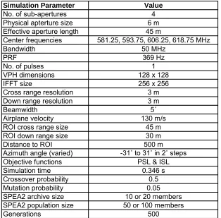
6.1 Scaled Scenario 1: SAR Mission... 47
6.1.1 Full Bandwidth, Single Aperture Experiment ...49
6.1.2 Split Bandwidth, Multiple Sub-Aperture Experiment ...58
6.2 Scaled Scenario 2: MTI Mission ... 67
6.2.1 Revisit Time & Integrated Pulses Experiment ...68
7 Conclusion and Future Work ...76
7.1 Conclusion ... 76
7.2 Future Work... 76
List of Abbreviations
AMTI Airborne Moving Target Indication CPI Coherent Processing Interval FFT Fast Fourier Transform GA Genetic Algorithm
GMTI Ground Moving Target Indication GUI Graphical User Interface
IFFT Inverse Fast Fourier Transform ISL Integrated Sidelobe Level
MOEA Multi-Objective Evolutionary Algorithm MOKP Multi-Objective Knapsack Problem MOP Multi-Objective Optimization Problem MTI Moving Target Indication
NGSA-II Non-Dominated Sorting Genetic Algorithm II pdf Probability Density Function
PRF Pulse Repetition Frequency PSF Point Spread Function PSL Peak Sidelobe Level PSR Point Source Response
ROI Region of Interest
SAR Synthetic Aperture Radar
SMRW Simultaneous Multi-Mission Radar Waveform SNR Signal-to-Noise Ratio
SPEA Strength Pareto Evolutionary Algorithm SPEA2 Strength Pareto Evolutionary Algorithm 2 TS Tournament Selection
List of Symbols
1
−
F Inverse Fourier Transform
∈ Belongs To
∀ For All
∃ There Exists
f Dominates
∨ Or
∧ And
List of Tables
Table 2-1: Requirements for radar missions of interest [13] ... 10 Table 6-1: Summary of simulation parameters for the full bandwidth, single aperture experiment... 50 Table 6-2: Summary of the evolution of PSL and ISL values for each full bandwidth, single aperture simulation ... 56 Table 6-3: Summary of simulation parameters for the split bandwidth, multiple sub-aperture experiment ... 60 Table 6-4: Summary of the evolution of PSL and ISL values for each split bandwidth, multiple sub-aperture simulation ... 65 Table 6-5: Single range cell fitness evaluation for revisit time & integrated pulses
List of Figures
Figure 2-1: A block diagram of a simple MTI radar [15]... 7
Figure 2-2: Simplified frequency response of a multiple pulse signal [5]... 8
Figure 2-3: Two-dimensional strip-map SAR scenario ... 12
Figure 3-1: Simple genetic algorithm flowchart ... 18
Figure 3-2: Example binary encoded individual... 19
Figure 3-3: Tournament selection... 22
Figure 3-4: Uniform crossover... 23
Figure 3-5: A mapping illustration from decision variable space to multi-objective function space (reproduced from [1] with author’s permission) ... 24
Figure 4-1: SPEA2 Flowchart... 30
Figure 4-2: Fitness assignment schemes for the same population in SPEA (left) and SPEA2 (right) [2]... 32
Figure 4-3: Illustration of the SPEA2 archive truncation scheme. N = 4 is assumed and the numbers on the right side indicate the order of elimination. ... 36
Figure 5-1: Binary encoded waveform suite... 40
Figure 5-2: RIT Multi-Mission Radar Waveform Tool: Selection of radar parameters GUI screenshot... 41
Figure 5-3: PSL SAR objective function. Absolute PSL values greater than 14 dB result in fitness values of 1. ... 43
Figure 5-4: ISL SAR objective function. Absolute ISL values greater than 45 dB result in fitness values of 1. Any absolute ISL value less than 20 dB gives a fitness value of 0. .. 43
Figure 5-5: Number of pulses MTI objective function. The target number of pulses (the number that gives a fitness value of 1) is the maximum allowed in the simulation scenario, 32. ... 44
Figure 5-6: Revisit time MTI objective function. The target revisit time is 0.75 s and results in a fitness value of 1. The maximum revisit time is 1.5 s and any value greater than 1.5 s results in a fitness value of 0. ... 45
Figure 6-1: Scenario 1 - SAR mission (not drawn to scale) ... 47
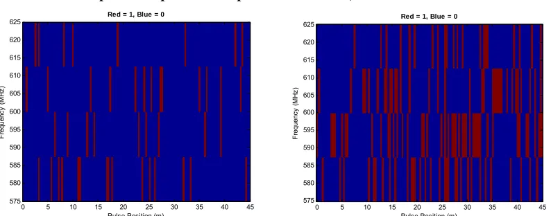
Figure 6-2: Example waveform suite for the full bandwidth, single aperture experiment49 Figure 6-3: Initial population and final archive population for the full bandwidth, single aperture experiment. Population Size = 50, Archive Size = 10. ... 52
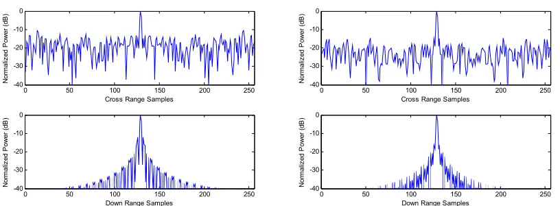
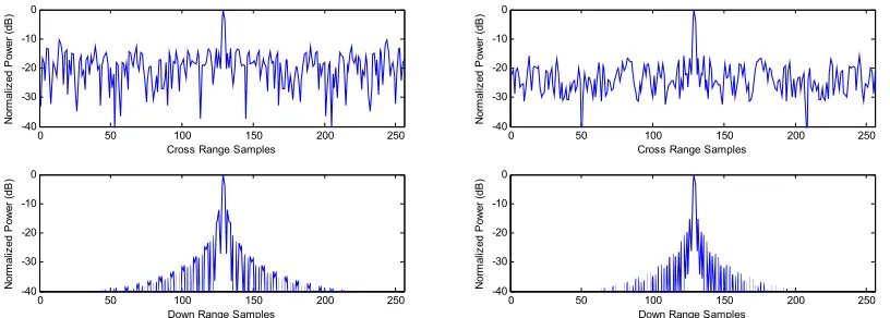
Figure 6-4: Initial (left) and final (right) VPH for the middle cell of the ROI. Population Size = 50, Archive Size = 10. ... 52
Figure 6-5: Initial (left) and final (right) PSR for the middle cell of the ROI. Population Size = 50, Archive Size = 10. ... 52
Figure 6-6: Initial population and final archive population for the full bandwidth, single aperture experiment. Population Size = 50, Archive Size = 20. ... 53
Figure 6-29: Initial (left) and final (right) PSR for the middle cell of the ROI. Population Size = 100, Archive Size = 20. ... 64 Figure 6-30: Initial population and final archive population using five different random seeds for the split bandwidth, multiple sub-aperture experiment. Population Size = 100, Archive Size = 10. ... 65 Figure 6-31: Archive population using five different random seeds for the split
bandwidth, multiple sub-aperture experiment. Population Size = 100, Archive Size = 10. ... 66 Figure 6-32: Scenario 2 - MTI mission (not drawn to scale)... 67 Figure 6-33: Example waveform suite for the revisit time & integrated pulses experiment ... 69 Figure 6-34: Initial population and final archive population for the revisit time &
integrated pulses experiment. Population Size = 50, Archive Size = 10. ... 71 Figure 6-35: Initial population and final archive population for the revisit time &
integrated pulses experiment. Population Size = 50, Archive Size = 20. ... 71 Figure 6-36: Initial population and final archive population for the revisit time &
integrated pulses experiment. Population Size = 100, Archive Size = 10. ... 72 Figure 6-37: Initial population and final archive population for the revisit time &
integrated pulses experiment. Population Size = 100, Archive Size = 20. ... 72 Figure 6-38: Initial population and final archive population for the revisit time &
1
Introduction
1.1
Objective
A radar is an electromagnetic system that operates by transmitting a particular type
of waveform and detecting the nature of the returned echo signal from reflecting objects
[3]. Radars are utilized for several different “tasks” often referred to as missions. Some of
these missions include ground moving target indication (GMTI), airborne moving target
indication (AMTI) and synthetic aperture radar (SAR) imaging. Current systems employ
mission-specific hardware and waveforms. There are some existing multi-mode radar
systems that have the ability to perform different missions [4], although not
simultaneously [1]. By reducing the amount of required hardware and containing a large
amount of information from a single waveform, a simultaneous multi-mission radar
platform would be the most efficient to date.
Different radar missions often have different objectives that may or may not be
related. The design of a radar waveform to accomplish such a mission forms a
multi-objective optimization problem (MOP). Often times, mission multi-objectives are conflicting
and are extremely difficult to effectively optimize. There are numerous radar parameters
that must be designed to successfully meet these objectives such as pulse repetition
frequency (PRF), center frequency, azimuth look angle, etc. The problem becomes even
more complicated when a multi-mission waveform design is considered. The number of
each mission. This type of optimization problem where the solution is not intuitive lends
itself well to evolutionary techniques.
Genetic algorithms (GAs) are a specific subset of evolutionary computation
techniques. They operate on the Darwinian concept of “survival of the fittest.” The
primary responsibility of the user is to define a fitness evaluation function that can
distinguish between “fit” and “unfit” solutions. When this is done effectively, genetic
algorithms have the ability to search a vast solution space for an “optimal” solution.
Achieving an “optimal” solution is the goal of every optimization algorithm, but
this raises the question of how one defines optimality. This becomes increasingly
complicated when a multi-objective scenario is considered. The Strength Pareto
Evolutionary Algorithm 2 (SPEA2), developed by Zitzler and Thiele [2], is a
multi-objective evolutionary algorithm that optimizes in a Pareto sense. A solution is Pareto
optimal (in the context of a maximization problem) if there exists no feasible vector
which would increase some criterion without causing a simultaneous decrease in at least
one other criterion [5].
In this thesis, SPEA2 is applied to the simultaneous multi-mission radar waveform
(SMRW) design problem. Waveform suites attempting to separately perform a
multi-objective SAR and a multi-multi-objective MTI mission are generated and evaluated by
SPEA2. The success of each mission is determined mathematically using a set of
objectives. Objective functions are developed to map mission performance to fitness
values that SPEA2 subsequently uses to determine a set of Pareto optimal solutions.
performance in a simulated environment. Some real world missions, such as SAR
imaging, operate over long periods of time (on the order of 20 minutes) and usually
involve a large region of interest (ROI). The scaled scenarios make it possible to evaluate
a complete family of Pareto optimal solutions in a reasonable amount of simulation time.
The results of numerous simulations demonstrating the fidelity of multi-objective radar
waveforms are presented. Finally, a true multi-mission, multi-objective scenario is
developed that requires the use of a parallel processing computer cluster in future
applications.
1.2
Literature Review for Multi-Mode/Multi-Mission Waveform
Design
By employing a frequency-diverse waveform generator and a sophisticated digital
signal processor, a single radar system capable of performing multiple missions can be
developed. These systems require an explicit selection of the radar mode of operation,
and then a specific waveform is generated to accomplish the selected mission. Many
current radar systems have multi-mode capabilities. Some of these systems are described
in [6], [7] and [8]. A perspective on the development of multi-mode radar systems is
given by Strong in [9]. Multi-mode capabilities are also being explored in space-based
radars, as discussed in [10].
One state-of-the-art multi-mode radar system is described in [4]. The AN/APG-76
multi-mode radar has the unique capability of performing SAR and GMTI missions
simultaneously using a multi-aperture antenna. It is important to note that this
different radars. Each aperture transmits its own mission-specific waveform to
accomplish its task. No multi-mode radar system can currently perform simultaneous
missions with a single waveform, which is the aim of this thesis.
There has been some previous research in the area of mode and
multi-mission radar waveform design and diversity. In [11], Mendelson and Ogle describe
many of the conflicting parameters for SAR and MTI missions. Their work focuses on a
processing technique that improves SAR and MTI mission capability for multi-mode
radar systems. Antonik et al. [12] proposed the concept of a frequency diverse array that
ignores the traditional separation of the antenna and waveform subsystems which
provides additional degrees of freedom for multi-mission applications. Their proposal
employs a separate waveform generator for each antenna which is controlled by its own
subsystem. Simultaneous multi-mission performance is not addressed by this work.
Amuso et al. [13] performed a systems analysis that demonstrates the difficulty in
designing a single radar system that can achieve SAR and MTI missions simultaneously.
Interleaved structure for multi-mission waveform design using a simple single-objective
genetic algorithm is discussed in this work. Interleaved waveform structure refers to
interspersing MTI waveforms with sections of SAR waveforms. This is not true
simultaneous multi-mission waveform design, as it is essentially a scheduling problem
for MTI and SAR waveforms. Due to the overly simple genetic algorithm and the
complexity of the problem, this approach did not produce worthwhile results.
The follow-up work from Amuso et al. employed a multi-objective genetic
simultaneous multi-mission waveforms [14]. Objective functions were used to evaluate
mission performance. Simultaneous multi-mission waveforms were designed for a
real-world scenario. Incremental increases in performance with respect to the defined mission
objectives were shown for the waveforms designed by SPEA with respect to randomly
generated waveforms. This thesis builds on the work presented in [14].
1.3
Outline
The organization of this thesis is as follows. Chapter 2 will describe the radar
missions of interest and note the difficulty in the design of a single waveform to
accomplish these missions. Chapter 3 will discuss genetic algorithms and will form the
multi-objective optimization problem. Chapter 4 will describe SPEA2 and note its
advantages over the other multi-objective optimization algorithms. Chapter 5 will detail
how SPEA2 is applied to the SMRW design problem. It will contain a description of the
desired missions to be accomplished as well as the objective functions used to evaluate
their success. Chapter 6 will describe the scaled real-world scenarios used for simulation
as well as provide the results and analysis of all experiments. Finally, Chapter 7 will give
2
Radar Background
2.1
Missions
The missions of interest for the SMRW design problem are synthetic aperture radar
(SAR) imaging and moving target indication (MTI). These missions are two of the most
common in radar application [15]. The following subsections will describe each mission
and its relevance to the SMRW design problem.
2.1.1 Moving Target Indication
Moving target indication (MTI) is one of the most common missions for a radar to
undertake. Separating moving targets from stationary ones is a vital task in many military
and security applications. MTI is an extremely important mission in high-quality
surveillance radars that operate in areas containing clutter [3]. For a stationary radar, an
MTI mission is carried out by measuring the Doppler frequency shift of the received
signal. A reference signal at the same frequency as the transmitted signal is utilized for
this Doppler shift measurement. A simple MTI radar is shown in Figure 2-1.
If the transmitted signal is of the form A1sin 2
(
π f tt)
, then the reference signal willbe of the same form with possibly a different amplitude, i.e. A2sin 2
(
πf tt)
. TheDoppler-shifted return echo that is received can then be represented as:
(
)
03
4
sin 2 t
echo t d
f R
V A f f t
c
π π
⎛
= ⎜ ± −
⎝ ⎠
⎞
⎟ (2-1)
where fdis the Doppler frequency shift, c is the velocity of propagation, and R0 is the
target range. Only the low frequency (fd) component of the echo signal is of interest, and
must be extracted.
A simplified frequency response of a multiple pulse signal is shown in Figure 2-2.
It has zero response at DC, which means that the radar will not detect stationary targets.
Also, because of the periodicity of the transmitted signal the response also rejects
frequencies in the vicinity of the PRF and its harmonics [3].
Figure 2-2: Simplified frequency response of a multiple pulse signal Error! Reference source not found.
The nulls in the frequency response are a significant issue with MTI radar systems which
radar cannot detect, due to its cancellation by the clutter rejection filter. Mathematically,
these blind speeds are given as:
( )
2 n
n PRF
v = λ (2-2)
An MTI mission becomes more difficult when the radar platform is in motion.
This is the case when the radar is aboard a flying aircraft, as was described in the SAR
mission. Clutter is not as easily distinguished when its Doppler frequency shift is no
longer equal to zero. However, this effect can be compensated for by one of two methods.
The first is to shift the frequency of the oscillator to account for the shift in the clutter
Doppler frequency [3]. The Doppler shift of the clutter is determined by the speed of the
aircraft and the pointing direction of the antenna. The other compensation method is to
redesign the FIR filter to reject the Doppler shift frequencies.
The design of a waveform to accomplish an MTI mission depends on the selection
of many parameters. The center frequency (fc) of the transmitted radar signal will
determine the Doppler frequency according to:
2 r c
d
v f f
c
= (2-3)
where vr is the relative radial velocity of the target with respect to the radar. The velocity
range that the radar is interested in detecting depends on what type of mission is to be
performed. Also, the range capability of a particular PRF must be considered. A
multiple-time-around echo is a signal that is received after an interval exceeding the pulse
repetition interval. These multiple-time-around echoes result in erroneous range
these multiple-time-around echoes, but as shown by Equation 2-2, it also produces a low
first blind speed. A high PRF introduces range ambiguities but also extends the first blind
speed so that faster moving targets can be detected. A GMTI mission must be able detect
slow moving targets, thus requiring a low PRF to ensure that no targets of interest fall
within the range of the blind speeds. In contrast, an AMTI mission must be able to detect
much faster moving targets, upwards of 700 m/s. This requires the use of a medium to
high PRF to extend the first blind speed and also to ensure that the target’s position is
frequently updated so that it is not lost. Table 2-1 [13] gives a summary of the conflicting
parameters needed to accomplish AMTI, GMTI, and SAR missions. The table contains
two parameters not previously discussed, dwell time and revisit time. Dwell time refers to
the total amount of time that a target is illuminated during a mission while revisit time is
the desired time between illuminations of a target during the mission.
Mission AMTI GMTI Stripmap SAR
Dwell Time (100 ms)Short Moderate (0.5 s) Very Long (20 min)
Revisit Time (~10 s)Short Moderate (30 s) Long
PRF (> 1 KHz)Medium (> 200 Hz)Low (~ 250 Hz)Low
Bandwidth (1 MHz)Narrow Moderate (5 MHz) (30 MHz)Wide
Beamwidth Narrow Narrow Wide
Table 2-1: Requirements for radar missions of interest [13]
When multiple pulses are transmitted from the radar, there are more opportunities
to detect and extract information from the echo signal. The likelihood that a target is
detected by a radar can be described by the following expression, known as the
( )
t
d sn
V
P p v d
∞
=
∫
v (2-4)Vt is the voltage threshold for detection and psn is the signal-plus-noise probability density
function (pdf) which depends on the signal-to-noise ratio as well as the signal and noise
statistics. Pd is a monotonic-increasing function of signal-to-noise ratio (SNR) for a given
threshold [15]. When many pulses are returned from a target, they can be summed to
improve the probability of detection. This process is called pulse integration. Pulse
integration can be done in two ways, before the threshold detection process (pre-detection
or coherent integration) or after the threshold detection (post-detection or non-coherent
integration) [3]. For ideal pre-detection, the SNR is improved by a factor equal to the
number of integrated pulses (M). For ideal post-detection, the SNR is improved by a
factor approximately equal to M as M becomes large [15]. Therefore, the number of
pulses that a radar emits upon each target is a critical factor for the detection of that
target.
MTI missions are a critical radar task, especially in military and air traffic control
applications [8], [9]. The detection and tracking of moving targets has become
increasingly important over the years [9]. Also imperative to military applications is the
ability to image an area. In some instances it may be critical to obtain images in high
resolution while others might require a system that can image through foliage. SAR
imaging can perform each of these tasks, among others, and thus is an important mission
2.1.2 Synthetic Aperture Radar Imaging
Synthetic aperture radar takes advantage of the motion of its carrier vehicle to
produce a high cross-range resolution. Effectively, the motion causes the synthesis of a
large antenna aperture. SAR achieves its high cross-range resolution by using the motion
of the vehicle to generate the antenna aperture sequentially rather than simultaneously as
with a conventional array antenna [3].
R θB
ROI v
v PRF
Figure 2-3: Two-dimensional strip-map SAR scenario
Figure 2-3 depicts a two-dimensional SAR scenario. The antenna is positioned to
transmit perpendicular to the direction of motion, which is referred to as sidelooking
radar or a strip-map SAR configuration. The X’s represent the positions at which a pulse
is emitted. ROI denotes the region of interest, θB is the antenna beamwidth, v is the
velocity of the aircraft, R is the range, and PRF is the pulse repetition frequency. The
effective aperture length (Leff) is equal to RθB.
There are two fundamental limits to the effective aperture length that can be created
(Leff ≤RθB). The second constraint is that the aperture size must be restricted so that the
phase front can be considered as a plane wave, also known as the far field of the array
[3]. The far field of an antenna is the minimum distance that the rays originating from a
radiating source may be considered parallel to each other at the target [3]. This far field
condition results in what is known as unfocused SAR. In unfocused SAR, the best
achievable resolution is a function of the square root of the range. However, if a
correction factor is applied that takes into account the curvature of the spherical
wavefront, the resolution can become independent of range. This phase correction factor
is defined as follows:
2
2 x
R
π ϕ
λ
Δ = (2-5)
where λ is the wavelength and x is the distance from the center of the synthetic aperture.
With this correction, all the received echo signals at range R are in phase and the SAR is
considered to be focused at this range. The cross-range resolution of the focused SAR is
2 cr
D
δ = (2-6)
where D is the size of the actual antenna. The down-range resolution is strictly a function
of the bandwidth (B)of the radar signal and can be approximated as follows [16]:
2 dr
c B
δ = (2-7)
where c is the wave propagation speed.
A SAR mission imposes constraints upon the PRF, just as an MTI mission does.
enough to avoid angle ambiguities (image fold-over) that result from too large a spacing
between the synthetic array elements. The distance traveled by the radar between pulse
transmissions should be less than half a wavelength [3]. This constraint places the first
grating lobe (θg) of the synthetic array at
( )
2 g
PRF v
λ
θ = (2-8)
Grating lobes are other maxima in a radiation pattern that are not the desired main beam.
They have the effect of producing undesired echo signals and thus usually should be
minimized or avoided [3]. It is known that the first null of the physical antenna (θn) is located at
n
D
λ
θ = (2-9)
Since θg ≥θn to avoid grating lobes, and combining Equations 2-6, 2-8 & 2-9, the lower
limit on the PRF is defined to be:
cr
v PRF
δ
≥ (2-10)
The upper limit on the PRF is imposed by the unambiguous range (Ru) constraint that was
previously discussed in Section 2.1.1. The PRF can not be greater than the amount of
time that it takes for a radar signal to travel to the target and back. Imposing this
constraint and combining with Equation 2-10 yields the range of PRF’s that can be
2
cr u
v c
PRF R
δ ≤ ≤ (2-11)
One technique to generate a SAR image is by first collecting a video phase history
(VPH). The cross-range dimension of the VPH contains spatial information while the
down-range dimension contains frequency information. Consider the problem of imaging
a region of interest (ROI) as depicted in Figure 2-3. The ground can be considered the
“target” in a terrain imaging application. As the radar travels along its path of motion, it
receives echo signals from the ground that differ in phase. This phase information is
stored as it is received at each position and effectively comprises the spatial information
in the cross-range dimension. It can be thought of as a discrete signal in the spatial
frequency domain, sampled at a rate equal to the velocity of the aircraft divided by the
PRF. The down-range dimension of the VPH is filled by indicating which part of the
frequency spectrum that the received signal belongs to. As noted by Equation 2-7, the
down-range resolution is determined by the bandwidth of the transmitted signal – i.e.
narrow pulses give high resolution. Narrow pulses are short in time which results in a
large frequency spectrum. This yields more bandwidth, and thus increased down-range
resolution.
The VPH generated by a SAR system can be represented in the frequency (ω - down-range) and spatial frequency domain (ku - cross-range) by the following equation:
(
2 2)
( , u) ( ) n( , u) ( , u) exp 4 u n
n
S ω k =Pω
∑
A ω k Aω k −j k −k x − jk yu n (2-12)where P( )ω is the Fourier transform of the transmitted radar signal, is the is Doppler
amplitude pattern for the nth target,
n
A
amplitude pattern, k is the wavenumber, xn is the down-range of the nth target, and yn is
the cross-range of the nth target. The SAR image is then reconstructed using
matched-filtered inversion as shown here:
* *
( , ), ( , ) ( ) ( , ) ( , )
x u y u u u
F k⎣⎡ ω k k ω k ⎤ =⎦ P ω A ω k S ω k (2-13)
The reconstructed image in the spatial domain is then obtained by applying a 2D inverse
Fourier transform as follows:
(
)
( , ) n n,
n
n
f x y =
∑
f x x y y− − (2-14)where
(
2)
1
( , )
( , ) ( ) ( , ) ( , ) x y
n k k u n u
f x y =F− P ω Aω k A ω k (2-15)
The nth target function f x yn( , ) is the point spread function (PSF) of the SAR imaging
system [16] and will be utilized to determine the quality of the SAR image in the
experiments to follow.
It has been shown that like an MTI mission, a SAR mission requires the
distinction of numerous parameters [1], [13]. The bandwidth of the transmitted signal is
directly related to the achievable down-range resolution of the SAR image, while the
cross-range resolution has an effect on the selection of PRF. It is of course desirable to
achieve the highest resolution possible, but constraints are imposed as shown in Equation
2-11 and also by other missions. The selection of the parameters such as PRF, center
frequency, number of pulses, bandwidth, etc. is where the challenge lies for
3
Genetic Algorithms & Multi-Objective Optimization
3.1
Genetic Algorithms
Evolutionary algorithms use the concept of “survival of the fittest” and
mathematically implement this concept into an algorithm in order to produce a generic
stochastic approach to solving single or multi-objective optimization problems [17].
Genetic algorithms are a specific subset of evolutionary algorithms that consist of
numerically encoded population members, commonly referred to as individuals1. Each
individual is represented by a number of genes that are grouped together to form
chromosomes. The information stored in the chromosomes is then extracted and
evaluated mathematically by an application-specific fitness function. This fitness measure
is then used to rank individuals within the population. At this point, a selection process is
applied to determine which members will pass to the next generation and be permitted to
produce offspring. This general process is repeated until the desired number of
generations is reached. A simple flowchart describing a basic genetic algorithm is shown
in Figure 3-1.
1
Initialize Population
Determine Fitness
Apply Selection Terminate?
Create Offspring
N
Y
Figure 3-1: Simple genetic algorithm flowchart
Genetic algorithms have the ability to explore many solutions throughout a vast
solution space. A genetic algorithm is a robust, stochastic search technique that has the
ability to evaluate a group of solutions in parallel and continuously refine them [18]. This
is the main characteristic of GAs that has made them so popular in a wide variety of
applications such as engineering [18] [19], finance [20], and computer science [21]
among others. The following sub-sections will describe each element of a genetic
algorithm in detail so that the reader is familiar with GA terminology and concepts before
SPEA2 is discussed.
3.1.1 Individual Representation & Initialization
To begin the discussion on the functionality of a typical GA, the numerical
representation of a single population member (individual) must first be addressed. From
an algorithmic point of view, the individual is nothing more than an encoded solution to a
mathematical problem [1]. Binary encoding of individuals was used for the radar
such as crossover and mutation are easily applied when binary encoding is used. An
example of a binary encoded individual is shown in Figure 3-2.
Figure 3-2: Example binary encoded individual
Each binary encoded gene represents a physical characteristic of the individual. A
collection of genes is known as a chromosome. As can be seen in Figure 3-2, both genes
and chromosomes can be of different lengths because there may be more bits needed to
encode one physical characteristic than another. The chromosomes contain the encoded
information that distinguishes each individual. The actual encoded values represented by
each gene are referred to as alleles [14].
To illustrate the aforementioned concepts, consider a human individual example,
as outlined in [1]. The nucleus of most human cells is comprised of two sets of
chromosomes, one coming from each parent. This results in 46 total chromosomes. These
chromosomes contain specific information about the individual. For an example, take eye
color. The gene that determines eye color is found in the same chromosome and position
for all humans. The value located in that particular position determines the actual color of
used for the encoding. For instance, say 00 – blue, 01 – brown, 10 – green, 11 – hazel.
Therefore, if the eye color gene was 01, the allele would be brown.
The genetic algorithm begins with the generation of an initial population (P0)
consisting of N individuals. This is usually accomplished by using a random number
generator. Once P0 is generated, each individual is evaluated by an application-specific
fitness function. It is at this point where the individual is decoded and mathematically
evaluated. This is the most crucial part of any GA. A fitness function that does not
effectively represent the desired characteristics for a solution will yield a poor result. The
fitness function for the SMRW design problem will be described in the following chapter.
For this discussion, it is not necessary to elaborate on how the fitness of an individual is
determined.
At this point, a common step is to rank the population members according to their
fitness. The ranking establishes order within the population. Depending on the fitness
function, this ranking can be done in ascending or descending order. Typically, most
genetic algorithms aim to increase fitness so descending ranking would be appropriate in
this case. This is usually the point in a GA where a check is performed to determine if the
maximum number of generations has been reached. If it has, then the algorithm
terminates and the current population (Pi) contains the possible solutions to the problem.
Because of the ranking process, the most “fit” individual is the first individual in the
3.1.2 Generating an Offspring Population
If the maximum number of generations has not been reached, the algorithm
continues and the offspring creation process is commenced. At this point, many GAs
employ a technique known as elitism. To ensure that the best solutions survive to the next
generation, X number of the most “fit” individuals are passed directly to the next
generation population (Pi+1). These X population numbers are usually referred to as the
“elite” members. This elitism technique has been shown to increase the performance of
GAs both mathematically [22] and empirically [23].
Next, mating pairs (or “parents”) must be selected from the population. There are
many different techniques that have been developed for this task. Some of these methods
include roulette wheel selection, rank selection, tournament selection and basic random
selection. Intuitively, a selection scheme that produces a balance between favoring the
traits of the best members and providing diversity by allowing many population members
to participate would most likely result in an effective search. For this reason, the mating
selection process that was chosen for the problem addressed by this thesis is tournament
selection (TS). TS provides the diversity that is needed to keep the population from
becoming stagnant by allowing all members to participate but it also favors the
individuals who possess higher fitness. The advantageous traits of tournament selection
including its speed and effectiveness are documented in [23]. TS begins by randomly
selecting four individuals from the current population, Pi. The four individuals are
grouped in pairs of two, and their fitness values are compared within these groups. The
process is repeated until the desired amount of mating pairs is achieved. A pictorial
representation of tournament selection is shown in Figure 3-3.
Ind. 22 – Fitness = 0.35 Ind. 11 – Fitness = 0.7
Ind. 4 – Fitness = 0.8 Ind.15 – Fitness = 0.4
Parent 1
Parent 2
Ind. 4 – Fitness = 0.8 Ind. 11 – Fitness = 0.7
Figure 3-3: Tournament selection
Once the parents are selected, a crossover operation occurs to create offspring.
There are also several crossover methods that can be implemented. Some of these include
single-point crossover, two-point crossover, and uniform crossover. Each technique is
inherently similar, as they all accomplish the same task of swapping genes between the
two parents. However, there are constraints to the single-point and two-point crossover
methods. In each technique, the crossover point must be selected at the beginning of a
gene. This constraint is imposed to ensure that the offspring population is a combination
of the physical characteristics of their parents. If this constraint was not met, the gene that
was split by the crossover would essentially be a mutation, meaning it may not be a trait
of either of the parents. Uniform crossover was chosen because it does not impose the
crossover point constraint. Uniform crossover selects a random number of genes to be
swapped between the two parents to create two offspring. Uniform crossover is illustrated
in Figure 3-4 where Gxy represents a binary gene. As can be seen in the figure, genes
shifting a gene’s position within a chromosome or changing the gene length. Any
crossover operation is usually subject to a crossover probability. This probability
determines the chance that two parent individuals will mate to produce offspring or
simply copy themselves as the offspring.
Parent 1 G11 G12 G13 G14 G15 G16 G17 G18 G19
Parent 2 G21G22G23G24G25G26G27G28G29
Offspring 1 G11G22 G G24 G G27 G
G12 G14 G17
13 15 G16 18 G19
Offspring 2 G21 G23 G25G26 G28G29
Figure 3-4: Uniform crossover
The number of offspring that are generated is algorithm specific. Generally, the
population size remains constant; therefore the number of offspring equals the population
size minus the elite population that was passed to the next generation. Before the
offspring proceed to the next generation, a mutation operator is often invoked to
introduce more variety in the search space. Binary mutation simply selects a random
number of bits that comprise the offspring’s genes to invert. A mutation probability is
used to determine how many bits are mutated. Typically, this is a small probability
because mutating many bits tends to make the GA perform more like a random search
technique [24]. At this point, the offspring population is combined with the elite
population and Pi+1 is complete. The Pi+1 population is then passed to the fitness
evaluation function and the process is repeated until the desired number of generations is
3.2
The Multi-Objective Optimization Problem
The Multi-objective Optimization Problem (MOP) can be defined as the problem
of finding a vector of decision variables which satisfies constraints and optimizes a vector
function whose elements represent the objective functions [25]. These objective functions
are often in conflict with one another and thus an ideal solution vector often times does
not exist. Pareto optimality defines a criterion to estimate the ideal solution and will be
discussed in the following section. First, the MOP and the ideal solution vector will be
defined mathematically.
Figure 3-5: A mapping illustration from decision variable space to multi-objective function space (reproduced from [1] with author’s permission)
Figure 3-5 illustrates the mapping of a solution (decision space) to a
multi-objective function space [1]. The MOP can be defined as follows:
Find a vector
[
]
Tn
x x x
x * *
2 * 1 *
... , , =
v (3-1)
which satisfies the m inequality constraints
m i
for x
and the p equality constraints
p i
for x
hi( )=0 =1,2,... (3-3)
as well as optimizes the vector function
( ) ( )
( )
[
]
Tk x f x f x f x
fv(v)= 1 v , 2 v ,... v (3-4)
In the context of the SMRW design problem, Equation 3-4 will be used to contain the
objective functions that map to the particular mission requirements. Now, let
[
Oi]
Tn i O i O i
O x x x
x () ()
2 ) ( 1 ) ( ... , , = v (3-5)
be a vector that optimizes the ith objective function. The vector
Ω ∈
) (i O
xv (3-6)
is such that
( )
x () opt f (x)f i
x i O
i v v
Ω ∈
= (3-7)
Thus the vector
[
O]
T k O O f f ff = 1 , 2 ,...
v
(3-8)
is ideal for a MOP. The point in Rn space that determines this vector shown in
Equation 3-8 is referred to as the ideal vector [1].
3.3
Pareto Optimality
When multiple, possibly conflicting, objectives are considered a compromise must
be attained in the optimization process. Pareto optimality, first introduced by Edgeworth
solution is Pareto optimal if there exists no feasible vector which would increase some
criterion (in a maximization problem) without causing a simultaneous decrease in at least
one other criterion [5]. To understand Pareto optimality, the concept of dominance with
respect to decision vectors must be defined. Consider two decision vectors, denoted vv1
and vv2 which belong to the solution set Ω. In context of a maximization problem, vv1 is
said to dominate vv2 if and only if
{
1, 2,...}
: i( )1 i( )2{
1, 2,...}
: j( )1 j( )i n f v f v j n f v f v
∀ ∈ v ≥ v ∧ ∃ ∈ v > v2 (3-9)
All decision vectors which are not dominated by any other decision vector of the solution
set are referred to as non-dominated [5]. Non-dominated decision vectors are considered
to be Pareto optimal. A collection of these non-dominated vectors is referred to as a
Pareto front. In the context of the MOP previously described, a vector is Pareto
optimal if for every and
*
xv ∈ Ω
x∈Ω
v I =
{
1, 2,...k}
either(
*)
( ) ( )
i I∈ f xi f xi
∀ v = v (3-10)
or there is at least one i∈I such that
*
( ) ( )
i i
f xv < f xv (3-11)
3.4
Evolutionary Multi-Objective Optimization Techniques
In the late 1960’s, genetic algorithms were beginning to be applied in
single-objective optimization problems. The first true multi-single-objective evolutionary algorithm
Genetic Algorithm (VEGA) [26] in the mid 1980’s. Since then, many different MOEAs
have been proposed, with only a certain few achieving noted success. Most successful
MOEAs incorporated David E. Goldberg’s ideas [27] on the use of non-dominated
ranking and selection to help guide solutions toward the Pareto optimal front. An
excellent review of the history of MOEAs is presented by Carlos A. Coello Coello in
[28]. An overview of two MOEAs noted in his article is presented in the following
subsections as a precursor to Chapter 4, which describes the Strength Pareto Evolutionary
Algorithm 2.
3.4.1 Strength Pareto Evolutionary Algorithm
Zitzler and Thiele introduced SPEA in the late 1990’s [5] and it quickly became
one of the most popular MOEAs because of its incorporation of elitism. SPEA utilizes an
archive of non-dominated population members which make up the elite population. Once
a member enters the archive, it is guaranteed to remain there until another solution comes
along that dominates it. Each individual in the archive is assigned a strength value that is
proportional to the number of solutions it dominates. Then, each individual in the
population is assigned a fitness value based on the strengths of the archive members that
dominate them. The archive size is limited in SPEA; if the archive grows larger than a
predefined limit a clustering technique is used that removes solutions that are located
close to one another in an attempt to preserve the characteristics of the Pareto front.
Mating pairs are chosen by using tournament selection on both the archive and the
SPEA was shown to perform well on a variety of multi-objective problems [5],
[29] and many of its characteristics were adopted by other techniques [30], [31].
However, as [31] would point out, SPEA contained some deficiencies that limited its
effectiveness in several instances. These deficiencies are addressed by SPEA’s authors in
the development of SPEA2.
3.4.2 Non-dominated Sorting Genetic Algorithm II
Kalyanmoy Deb et al. introduced the Non-dominated Sorting Genetic
Algorithm II in 2000 and published it in 2002 [31]. This algorithm implements a fast
population ranking scheme which reduces its computational complexity compared to
most other MOEAs. Also, rather than employing the fitness sharing technique proposed
in its first version [32] to promote diversity in the population, NSGA-II uses a
crowded-comparison operator to accomplish this task. Fitness sharing requires a user-defined
sharing parameter, often denoted σshare, which determines the amount of sharing desired
in the problem. The diversity of the population is heavily dependent on this sharing
parameter and it is often unclear what value it should take. NSGA-II defines a “crowding
distance” ( ) measure which computes the average distance of two points on either
side of the individual in question along each objective. The selection process takes into
account the number of individuals that each member dominates (referred to as
non-domination rank, denoted ) as well as the crowding distance measure. The guiding of
the selection process is outlined using the crowded-comparison operator ( ) as follows:
distance
i
rank
i
n
p
( ) (( ) ( ))
n rank rank rank rank distance distance
Equation 3-12 states that between two solutions with different non-domination ranks, the
solution with lower rank is preferred. If the non-domination ranks are equal, the solution
belonging to a less crowded area is desired.
NSGA-II has been shown to produce very promising results on standard
multi-objective test problems [2] [31], prompting its inclusion as one of the landmarks for
evaluating other MOEAs. It was also shown to be superior to SPEA in almost every
measurable fashion. This prompted Zitzler, Thiele and Laumanns to develop its own next
4
The Strength Pareto Evolutionary Algorithm 2
(SPEA2)
4.1
Overview
The Strength Pareto Evolutionary Algorithm 2 [2] presents several improvements
over its predecessor SPEA. It boasts an improved fitness assignment scheme which
distinguishes individuals in a much more effective fashion. A more precisely guided
search process is fostered by a nearest neighbor density technique. Finally, a new archive
truncation method guarantees the preservation of boundary solutions to ensure that the
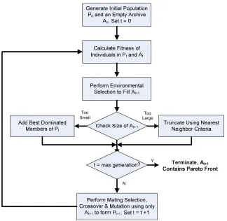
[image:43.612.166.490.368.684.2]Figure 4-1 depicts the flowchart for SPEA2. An initial population is created by
using a random number generator, as was described in Section 3.1.1. An archive of elite
solutions, denoted At where t is the generation number, is utilized in SPEA2 as in SPEA
to preserve the best solutions across each generation. However, unlike its predecessor, the
archive size in SPEA2 is constant. Also in contrast to SPEA, SPEA2 selects mating pairs
only from the archive population. This promotes the reproduction of advantageous
characteristics, but at the same time limits the variation in the offspring. Variation can be
introduced through the mutation operator. The user decides what type of mating
selection, crossover operation, and mutation operator to implement. For the SMRW
design problem, tournament selection, uniform crossover, and binary mutation were
employed as described in Section 3.1.2.
The details of SPEA2 will be described in the following sections. Section 4.2 will
discuss the fitness assignment scheme which includes the nearest-neighbor density
technique. Section 4.3 will describe the environmental selection process as well as the
techniques used to maintain a constant archive size.
4.2
Fitness Assignment
One of the deficiencies that was discovered in SPEA was that individuals who
were dominated by the same archive members were assigned identical fitness values. It
was irrelevant if one dominated member performed better than the other dominated
member in each objective. Both dominated members had equal probability of passing to
search algorithm. Therefore, in SPEA2, each individual’s fitness is based upon the
solutions that dominate it as well as the solutions that it dominates.
For each individual i, a strength value S(i) is determined that represents the
number of solutions that it dominates. In mathematical terms,
{
}
( ) | t t
S i = j j P∈ +A ∧if j (4-1)
where | | denotes the cardinality of a set and + represents a multi-set union. These
strength values are then used to assign a raw fitness, R(i), to each individual.
,
( ) ( )
t t
j P A j i
R i S
∈ +
=
∑
jf (4-2)
Thus, the raw fitness of an individual is determined by the strength of its dominators in
both the archive and the population [2]. Note that in terms of raw fitness, a low number
represents a “good” solution, i.e. it is not dominated by many members. A zero raw
fitness would indicate that the particular individual is non-dominated. This idea is
illustrated in Figure 4-2 along with a comparison of SPEA’s fitness assignment scheme.
Figure 4-2: Fitness assignment schemes for the same population in SPEA2 (left) and SPEA2 (right) [2].
2
It is imperative to understand the difference between fitness assignment strategies
between SPEA and SPEA2. In Figure 4-2, the letters are used to distinguish between
population members for the purpose of this discussion. SPEA’s fitness assignment begins
by determining the number of solutions that each archive member dominates. In the case
depicted by Figure 4-2, there are three non-dominated members (A,B,C) which make up
the external archive population and three population members (D,E,F). Members A and C
dominate one member: F, while member B dominates three members: D, E, and F. These
domination counts are then divided the number of population members (3) plus one to
produce a fitness value for the archive members. The population members are then
assigned a fitness value equal to the summed fitness values of its dominators plus one.
Members D and E are dominated by B, therefore their fitness values are both equal to
member B’s fitness plus one – i.e. 3/4 + 1 = 7/4.
The SPEA2 raw fitness assignment scheme utilizes a strength value (S) and a raw
fitness value (R). The strengths of each member are equal to the number of individuals in
the population that they dominate and the raw fitness values are equal to the sum of the
strengths of each member’s dominators. The non-dominated members (A,B,C) have a
raw fitness value equal to 0 because they are not dominated by any other member.
Members A and C dominate one member, F, so their strength is equal to 1. Member B
dominates 3 members (D,E,F) so its strength value is 3. Member D is only dominated by
member B, so it is assigned a raw fitness value of 3. It dominates members E and F, so it
is assigned a strength value of 2. This assignment process continues for each member of
Figure 4-2 explicitly shows the deficiency of the SPEA fitness assignment
scheme. The two individuals that are dominated by the same member of the archive
population (D and E) are assigned the same fitness value (7/4), despite the fact that one
individual (D) is clearly superior to the other (E) in objective space. The SPEA2 fitness
assignment remedies this issue. Individual D has a lower raw fitness (3) than individual E
(5), indicating that it is indeed a better solution.
Raw fitness is only one part of the SPEA2 fitness measure. To differentiate
between individuals that may, by chance, have identical raw fitness values, an additional
density measure is incorporated. The inverse of the distance to the k-th nearest neighbor
is taken to be the density estimate for a given individual. For every member, the distances
to all other members is calculated and sorted in ascending order. The distance to the k-th
element, denoted σik, is the point of interest for the density measure. Based on the work
of Silverman in [33] the SPEA2 authors determine k as follows:
( ) ( )
k = size P +size A (4-3)
The density for each individual is then calculated as:
1 ( )
2 k i
D i
σ =
+ (4-4)
Two is added in the denominator to ensure that D(i) takes a value less than one. Finally,
the fitness of an individual for the SPEA2 algorithm is calculated as:
( ) ( ) ( )
4.3
Environmental Selection
The process by which the archive population is updated and maintained is referred
to as environmental selection. For SPEA2, the first step of this process is to copy all
non-dominated individuals from the current archive and population to the next generation’s
archive (i.e. At+1). Non-dominated individuals are easily distinguished, as they are
guaranteed to have a fitness value less than one. This update process is depicted
mathematically by:
{
}
1 | (
t t t
A+ = i i P∈ +A ∧F i) 1< (4-6)
At this point, the size of the archive is checked against the pre-defined size limit,
denoted N. If then the environmental selection process is complete and
mating selection can be commenced. If
1
( t )
size A+ =N
1
( t )
size A+ < N then the archive is filled with the
best dominated population members (an easy task given that the members are already
sorted in ascending fitness). The most complicated situation occurs when size A( t+1)>N.
When the size of the archive is larger than N, the SPEA2 truncation operator must
be utilized. This algorithm iteratively removes solutions from the archive until it meets
the size requirement. This is accomplished by choosing the individual which has the
minimum distance to another individual at each stage. Ties are broken by the second
smallest distance, etc. The goal of this truncation technique is to maintain the spread of
the Pareto front while also preserving the boundary solutions. The technique is illustrated
(
)
1
1
: 0 ( ) :
0 ( ) : 0 :
k k
d t i j
l l k k
t i j
i j k size A
k size A l k
σ σ
σ σ σ σ
+
+
≤ ⇔ ∀ < < = ∨
i j
⎡ ⎤
[image:49.612.173.505.86.377.2]∃ < < ⎣ ∀ < < = ∧ < ⎦ (4-7)
Figure 4-3: Illustration of the SPEA2 archive truncation scheme. N = 4 is assumed and the numbers on the right side indicate the order of elimination.
As Figure 4-3 depicts, the first solution that is truncated from the Pareto front is the
one that is closest to its nearest neighbor (B). Notice that member A is not removed
because it is a boundary solution. Member G will also not be removed in any truncation
scenario. The second elimination is made as a decision between members E and F. They
are the two members with the minimum distance to each other. Member F is selected to
be removed because the distance to its next nearest neighbor (G) is smaller than member
E’s next nearest neighbor (D). The archive size is set to be four, so one more solution
must be removed. The next minimum distance between two members is between C and
D. Member D is chosen to be removed because the distance from D-E is smaller than the
4.4
Verification with the 0/1 Multi-Objective Knapsack Problem
To verify the functionality of the SPEA2 implementation, the 0/1 multi-objective
knapsack problem (MOKP) was utilized [34]. The standard 0/1 single objective knapsack
problem is well-known and is frequently used to test optimization algorithms. It is a
combinatorial optimization problem in which a set of n items each have an associated
profit (p) and weight (w). The goal of the experiment is to choose the items that have the
maximum profit while not exceeding the weight capacity (W) of the “knapsack.”
Mathematically, this is stated as follows:
{ }
1 1
0,1 1
n n
j j j j
j j
j
maximize p x subject to w x W
x for all j n
= =
≤
∈ ≤ ≤
∑
∑
(4-8)
To extend this into a multi-objective problem, m knapsacks with different weight
capacities are introduced. When an item is selected for inclusion, it is placed in all m
knapsacks. The items also have knapsack-specific profits and weights, corresponding to
the effects of including an item on each objective. The 0/1 MOKP is defined as follows:
{ }
1 1
1
0,1 1
n n
i j j ij j i
j j
j
maximize p x subject to w x W i m
x for all j n
= =
≤ ≤ ≤
∈ ≤ ≤
∑
∑
(4-9)
Zitzler and Thiele have developed a comprehensive set of MOKP test data and
results3 that are referenced in [2], [5] and [29]. For the purposes of verifying the
functionality of the SPEA2 implementation, a simple MOKP was chosen for testing. A
three knapsack, one-hundred item problem was selected. This problem was robust
3
enough to exercise SPEA2 but simple enough to accomplish given the computational
constraints. A population size of five-hundred members was used along with an archive
size of 30, per the experiments in [2]. Although the problem could not be evolved for as
many generations as in [2] (50 as opposed to 500), the results were similar to those
reported by Zitzler and Thiele. This indicated that the algorithm was indeed functioning
5
SPEA2 Applied to Simultaneous Multi-Mission
Radar Waveform Design
5.1
Waveform Suite Approach
Section 1.2 noted the main deficiency of existing multi-mode radar systems: they
cannot accomplish multiple missions simultaneously using the same waveform. Section
2.1 highlighted the numerous radar parameters that are of specific interest to
accomplishing MTI and SAR missions, some of which are summarized in Table 2-1. This
section will aim to define a single waveform, which will be referred to as a waveform
suite, that combines different radar parameters to accomplish multiple missions
simultaneously.
The RIT Multi-Mission Radar Waveform Tool has been developed in MATLAB®
and provides its user the ability to vary a number of different radar parameters. These
parameters are:
• N