Matched wavelet construction and its application to target detection

Rochester Institute of Technology

RIT Scholar Works

Theses

Thesis/Dissertation Collections

8-25-1995

Matched wavelet construction and its application

to target detection

Joseph Chapa

Follow this and additional works at:

http://scholarworks.rit.edu/theses

This Dissertation is brought to you for free and open access by the Thesis/Dissertation Collections at RIT Scholar Works. It has been accepted for

inclusion in Theses by an authorized administrator of RIT Scholar Works. For more information, please contact

[email protected].

Recommended Citation

Dr. Mark Fairchild, Coordinator, Ph.D. Degree Program

Matched Wavelet Construction and Its

Application to Target Detection

by

Major Joseph O. Chapa, USAF

B.S. Illinois College (1981)

B.E.E. Auburn University (1983)

M.S. Stanford University (1986)

A thesis submitted in partial fulfillment of the

requirements for the degree of Ph.D. in the

Center for Imaging Science

Rochester Institute of Technology

August 25, 1995

Signature of the Author

_

Jo§eph O. Chapa

Accepted

by

--J~!~~__=__.>.~I1__.:.'1_=____J

CENTER FOR IMAGING SCIENCE

ROCHESTER INSTITUTE OF TECHNOLOGY

ROCHESTER, NEW YORK

CERTIFICATE OF APPROVAL

Ph.D. DEGREE DISSERTATION

The Ph.D. Degree Dissertation of Joseph O. Chapa

has been examined and approved

by

the

dissertation committee as satisfactory for the

dissertation requirement for the

Ph.D. degree

in

Imaging Science

Dr. Mysore Raghuveer, Thesis Advisor

Dr. Edwin Hoefer

Dr. Harvey Rhody

THESIS RELEASE PERMISSION

ROCHESTER INSTITUTE OF TECHNOLOGY

CENTER FOR IMAGING SCIENCE

Title of Thesis: Matched Wavelet Construction and Its Application to Target Detection

I, Joseph O. Chapa, hereby grant permission to the Wallace Memorial Library of

R.I.T.

to reproduce

my thesis in whole or

in

part. Any reproduction will not be for commercial use or profit.

Signature:

_

<::7/25/15

ACKNOWLEDGEMENTS

I

wish to acknowledge

my Sovereign God for his love

and provision and

for faith in

Christ

which

He

worked

in

me and

for

the

hope

that

He

gave me

from

the

first

day

of

this

schoolassignment, through

every

obstacle and

every

success.

I

wishto thank

my

loving

wife,

Debbie,

for her

patience,

love,

support, and encourage

ment

during

thecourse

of

this

Ph.D.

program.

I

would also

like

to thank

my

children,

Katie,

Joey, Frank,

and

Becky

for

their

love

and

understanding

even

during

times

of

stress

in

their

Dad's

life.

I

wishto thank

my

advisor,

Dr. Mysore

Raghuveer,

for

his

patience, guidance,

and

knowl

edgeas

he helped

me through

my

researchandfor

teaching

me,

by

example,

the

difference

between

a student andascholar.

I

wishto thank

my

committee,

Dr. Edwin

Hoefer,

Dr.

Harvey

Rhody,

and

Dr. Navalgund

Abstract

This

dissertation develops

a new wavelet

design

technique thatproduces a waveletthatmatchesa

desired

signal

in

the

least

squaressense.

The Wavelet Transform lias become

very

popular

in

signal and

image

processing

overthe

last 6

years

because it is

a

linear

transformwith an

infinite

number

of

possible

basis

functions

thatprovides

localization in both

time

(space)

and

frequency

(spatial frequency).

The Wavelet Transform is very

similarto thematched

filter

problem, wherethewaveletactsas a zero mean matched

filter. In

pattern recognition applications wherethe output

of

the

Wavelet Transform is

to

be

maximized,

it is necessary

to use wavelets thatare

specifically

matchedto the signal

of

interest.

Most

current wavelet

design techniques,

however,

do

not

design

thewavelet

directly,

but

rather,

build

a composite wavelet

from

a

library

of previously designed

_wavelets,

modify

the

bases in

an

existing

mul-tiresolutionanalysis or

design

a multiresolution analysisthat

is

generated

by

a

scaling function

which

has

a specific

corresponding

wavelet.

In

this

dissertation,

an algorithm

for

finding

both

symmetric and asymmetric matched wavelets

is developed. It

will

be

shownthatundercertain_{conditions, the}matched waveletsgenerate an orthonormal

basis of

the

Hilbert

space

containing

all

finite energy

signals.

The

matched orthonormal wavelets give risetoa pair

of Quadrature Mirror Filters

(QMF)

thatcan

be

used

in

the

fast Discrete Wavelet Transform.

It

will also

be

shown thatas the conditions are relaxed, the

algorithm produces

dyadic

wavelets which when used

in

the

Wavelet Transform

provides significant re

dundancy

in

the transform

domain.

Finally,

this

dissertation develops

a

shift,

scale and rotation

invariant

technique

for

detecting

an

Contents

1

Introduction

1

2

Background

4

2. 1

Hilbert Spaces

4

2.2

Fourier

Analysis

7

2.3

Wavelet

Analysis

12

3

Wavelet

Theory

Development

15

3.1

Continuous

Wavelet Transform

15

3.2

Dyadic Wavelets

20

3.3

Frames

21

3.4

Orthonormal Wavelets

23

3.5

Multiresolution Analysis

24

3.5.1

Properties

ofcj>and

ip

30

3.6

Discrete Wavelet Transform

33

3.7

2-Dimensional DWT

42

3.8

Limitations

to the

MRA

and

DWT

45

3.8.1

MRAs

45

3.8.2

DWT

45

4

Wavelet Design Techniques

48

4.1

Compactly

Supported Wavelets

48

4.2

Wavelets for Signal Representation

51

4.3

Entropy-Based Best Basis Selection

52

4.4

Matching

Pursuit

with

Time-Frequency

Dictionaries

53

4.5

Multiresolution Analysis-type Wavelets

54

4.6

Biorthogonal Wavelets: The

Lifting

Scheme

57

5

Matching

a

Wavelet

to

a

Signal

60

5.1

Motivation: Signal Detection

60

5.2

Orthonormal MRAs

62

5.3

Matching

a

Wavelet

toa

Signal

64

5.3.1

Finding

the

scaling function from

a wavelet

64

5.3.2

Properties

of

the

wavelet spectrum amplitude

66

5.3.3

Matching

Spectrum Amplitudes

68

5.3.4

Properties

of

the

wavelet spectrumphase

69

5.3.5

Matching

Spectrum Phase

73

5.4

Generating

Matched Wavelet Frames

74

6

Examples

79

6. 1

Orthonormal Wavelets

79

6.1.1

Meyer's

Wavelet

80

6.1.2

Gabor's Wavelet

84

6.1.3

Daubechies'

D4

wavelet

88

6. 1

.4

Transient

signal

94

6.2

Dyadic Wavelets

100

6.2.1

Gabor's Wavelet

100

7

Applications

to

Image

Object Detection

105

7.1

The Radon Transform

105

7.2

Image Reconstruction

and

Backprojection

108

7.2.1

Reconstruction

by

direct Fourier Methods

108

7.2.2

Reconstruction

by

backprojection

109

7.3

The Wavelet Radon Transform

110

7.4

Matched Wavelets

and

Object Detection

115

7.4.1

Training

ona

Known Object

115

7.4.2

Object Detection

125

7.4.3

Detection Results for

an

Unknown Object

131

8

Summary

139

8.1

Future Research

140

8.2

Conclusion

140

List

of

Figures

2. 1

Orthonormal

projection

6

2.2

Short-Time

Fourier Transform

10

2.3

Time-frequency

map

-Short Time Fourier Transform

11

2.4

Time-scale map

-Wavelet Transform

14

3.1

The Gabor

or

Morlet

wavelet

17

3.2

Continuous Wavelet Transform

of atransientsignal

19

3.3

Multiresolution Decomposition

ofL2

(3?)

26

3.4

N-

level

Multiresolution Decomposition

28

3.5

Daubechies'

D4 Wavelet

and

Scaling

Function

28

3.6

Multiresolution Decomposition Example using

the

D4

wavelet

29

3.7

Discrete Wavelet Transform

35

3.8

Discrete

Multiresolution Decomposition

oftransientsignal

D4 filters

37

3.9

Decomposition/Reconstruction

cycle with

QMF filters

38

3.10

DWT Decomposition/Reconstruction

-

Effects

_onthe

Signal

Spectrum, a) Original

Signal;

b)

Spectrum

of

H

and

G;

c) Spectrum

ofCj~l and

D''1;

d)

Spectrum

ofC^1 and

D'-1;

e)

Spectrum

ofC^'"1 and

>j_1;f)

Spectrum

ofCjand

Dj;

g) Spectrum

ofCj

39

3.11

2-D Multiresolution Decomposition

43

3.12

Multiresolution

Decomposition

of

Lena

Using

Daubechies'

D4 Wavelet

44

5.1

Algorithm

Flow Chart

75

6. 1

Constraint

Matrix

-

A

for 2n/3

<

u <

87r/3

80

6.2

Construction

oftheconstraint matrix

A

81

6.3

Meyer's

wavelet

82

6.4

Amplitude Match in

thepassband-

Meyer

83

6.5

Meyer's scaling function

83

6.6

Gabor's

wavelet

84

6.7

Gabor's

spectrum and poisson summation

85

6.8

Amplitude

match

in

thepassband

-Gabor's

wavelet

85

6.9

Matched

wavelet spectrum and poisson summation

-Gabor

86

6. 10

Scaling

function

spectrum and poisson summation-

Gabor

86

6.11

Matched

wavelet vs

Gabor's

wavelet

87

6.12

Scaling

function

-Gabor

87

6.13

Daubechies'

D4 Wavelet

and

Scaling

Function

88

6.14

Truncated Spectrum

and

Poisson

Summation

-

D4

89

6.15 Amplitude

Match

in

thepassband

-D4

89

6.16

Matched Wavelet Spectrum

and

Poisson Sum.

D4

90

6.17

Scaling

Function Spectrum

and

Poisson Sum.

D4

90

6.18

Matched Wavelet

Group Delay

vs

desired

-

D4

91

6.19

Scaling

Function

Group

Delays: Derived

vs

Truth

-

D4

92

6.20

Matched Wavelet

and

Scaling

Function

vs

desired

-

D4

93

6.21

QMF

filters

g(k)

and

h(k)

-

D4

93

6.22

Transient Signal

94

6.23

Desired Signal Spectrum

and

Poisson

Sum

- transient

95

6.24

Amplitude Match in

thepassband- transient

95

6.25

Matched Wavelet Spectrum

and

Poisson

Sum

-transient

96

6.26

Scaling

Function

Spectrum

and

Poisson Sum

6.27 Matched

Wavelet

Group

Delay

vs

desired

-transient

97

6.28

Matched Wavelet

vs

desired

signal

-transient

97

6.29

Scaling

Function

-transient

98

6.30

QMF filters g(k)

and

h(k)

- _transient

99

6.31

Constraint

Matrix

-

A

for 0

< u> <

4ir

100

6.32

Amplitude Match in

theextended passband-

Gabor

101

6.33

Matched Dyadic Wavelet

vs

Gabor's

wavelet

101

6.34

Matched Dyadic

wavelet spectrum and poisson summation-

Gabor

102

6.35

Amplitude Match in

theextended passband-

D4

103

6.36

Matched Dyadic

wavelet spectrum and poisson summation-

D4

103

6.37

Matched Dyadic Wavelet

vs

D4

wavelet

104

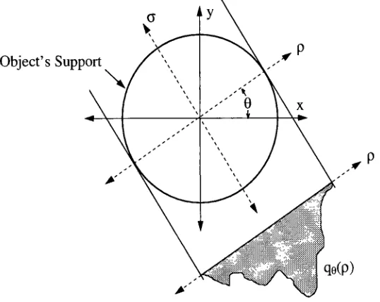
7.1

Projection geometry for

tomographic

processing

106

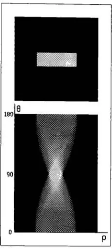
7.2

Radon Transform

of a rectangle

image

107

7.3

Projection Slice Theorem

109

7.4

Backprojection

ofqg

(p)

110

7.5

Image Reconstruction using

the

Backprojection Algorithm

...

Ill

7.6

Geometry

for

the

Wavelet Radon Transform

Ill

7.7

Image

of a rectangular object

112

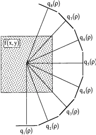
7.8

Projections

of rectangle

image

at

8 equally

spaced angular

intervals

113

7.9

Wavelet

Radon Transform

of rectangle

image using

the

D4

wavelet

114

7.10

Training

Procedure for Object Detection

116

7.11

Training

image

of

fighter

aircraft

117

7.12

Projections

of

fighter

aircrafttakenat

8

equally

spacedangles

118

7.13

Dilated

projections andtheirassociatedmatchedwavelets

-pass

0

119

7.14

Wavelet Radon Transform

of

jet

aircraft projections- _pass

0

120

7.15

Peak

values

from

the

WRT

-matchedwaveletsvs

Meyer's

wavelet

122

7.16

Projections

andtheirestimate

7.17

Dilated

projections andtheirassociated matchedwavelets

-pass

1

124

7.18

Projections

andtheirestimate

-pass

1

125

7.19

Object Detection Algorithm

126

7.20

Normalized Circular

Correlation,

s -0

128

7.21

Results

of

backprojected detection

and

detail

signals -0

130

7.22

Test image

for

detection

131

7.23

Projections

andtheirestimate- _test

image,

_pass

0

132

7.24

Wavelet Radon Transform

of

Test

image

projections

-pass

0

133

7.25

Normalized Circular

Correlation,

s-

Test image

134

7.26

Results

of

backprojected

detection

and

detail

signals-

Test

image

136

7.27

Wavelet Radon

Transform

of

Test image

projections

-pass

1

137

7.28

Test

image

projections andtheirestimate

List

of

Tables

6.1

h(k)

for

ip

matchedto

fD

^

Chapter 1

Introduction

For many

years, the

primary linear

mathematical analysis

tool

used

to transform

signal

information

was

the

Fourier Transform.

However,

the

end ofthe

1980's

saw

the

development

of an alternative mathe

matical

framework,

called the wavelet

transform,

withapplications

in

signal and

image

analysis

[30].

While

much of

the

theory

associated with

it is

not newand can

be described in

a

Hilbert

space

setting,

it did

provide a consolidated

framework for

a number of

previously diverse

disciplines,

like

multireso

lution

analysis used

in

computer

vision,

subband

coding developed for

speechand

image

compression,

and orthonormal

basis

expansions

developed in

applied mathematics

[30].

The Fourier Transform

of a

signal,

f{x),

given

by

/oo

f{x)e~wxdx,

(1.1)

-oo

is

a projection operation onto

the

basis formed

by dilating

the

complex

exponential,

elx.

The Wavelet

Transform,

given

by

f{x)\a\-3ii>[^-)dx,

(1.2)

is

aprojection operationontothe

basis formed

by dilating

and

shifting

a"mother"wavelet, ip(x),which

is

zeromeanand

decays very rapidly in

x.

These

properties of

the

wavelet provide an advantage over

Fourier

analysis

because

the

Wavelet Transform

canachieve

localization

in both

time

and

frequency

or

in

the

case of

images,

space and spatial

frequency

[10]. That

is

to

say

that the

Wavelet

Transform

can

waveletanalysisover

Fourier

analysis

is

the

flexibility

in

the

transform

operator used

for decomposition

orsignal representation.

Fourier

methods are

locked into bases

that

are

based

on

the

complexexponential

kernel,

e8x.

Wavelet

transforms

can

have

many different

operators.

They

may

or

may

not

be

orthogonal,

and

they

may

or

may

not

form bases. Even in

the

case of orthonormal

bases,

there

are still

infinitely

many

wavelets

that

satisfy

the

appropriate conditions.

Because

of

this

flexibility,

it is

possible,

and

wise, to

choose or

design

a wavelet

that

is

matched

to the

application.

Many

wavelet

design

techiques

have been

developed

since

the

early

theoretical

workof

the

wavelet

pioneers.

However,

mostof

the techniques

do

not

directly

match a wavelet

to

a signal of

interest.

Many

build

adaptive wavelets

from existing

wavelets and

their

effectiveness

is dependent

on

the

effectiveness

of

the

existing

wavelets used.

Others

impose

requirements on

the

wavelets

to

ensure some

degree

of

smoothness or

differentiability,

which guarantees

the

wavelet

to

exhibit certain

properties,

but does

not

guarantee

anything

withregards

to

its

shape.

Using

adaptive wavelets

for image

pattern recognition

is very

attractive

because

of

the

scale

(or

zoom)

insensitivity

of

the

wavelet

transform.

For

instance,

if

a wavelet can

be

constructed

that

matches

a pattern of

interest in

an

image,

then the

peak ofthe wavelet

transform

(or

lack

thereof)

will

indicate

whether

the

pattern

is

present

(or

not)

and

due

to the

localization

properties of

the wavelet,

where

the

pattern

is located.

Applying

the

Continous Wavelet Transform

(CWT)

to the

image

would

be

too

data

intensive because

of

the

redundancy

contained

in

the

CWT. The 2-D Discrete Wavelet

transform

is

much

faster because it

processes

the

projection coefficients only.

However,

it is

not shift or rotation

invariant,

making

its

application

to

pattern recognition of

limited

use.

These

two problems,

wavelet

matching

and application

to

pattern recognition are addressed

in

this

dissertation.

First,

a wavelet

design

algorithm

is developed

that takes

any 1-D

signal as

input

and

finds

the

wavelet

that

comes closest

to

it in

the

least

squares sense.

The

algorithm assumes

that the

wavelet

is bandlimited. The bandlimit

conditions can

be

set such

that the

resultant wavelet

is

an orthonormal

basis

of

the

function

space

L2(Jr.),

or

they

can

be

relaxed or

widened,

so

that the

algorithm generates

a"dyadic"wavelet.

Second,

a

target

detection

and

identification

algorithm

is

developed based

on

the

detec-tion

algorithm

is

shift,

scale and rotation

invariant.

The Radon Transform is

used

to

reduce

the

data

burden

on

the

CWT

and

to

provide some

degree

of rotation

invariance.

Using

matched wavelets

in

the

CWT

provides scale and shift

invariance

aswellasoptimalamplitude

detection.

The

matched wavelet

algorithm

in

conjunctionwith

the

target

detection

algorithm provide a

thorough

framework from

which

more

detailed

target

classification algorithms could

be

developed.

This

dissertation

provides an

in-depth

reviewofwavelet

theory,

first in Chapter 2

with a short review

of

Hilbert

spaces and a comparison

between Fourier

and

Wavelet

analysis.

Chapter 3

provides an

histor

ical chronology

of

the

development

of wavelet

theory

from

the

Continuous

Wavelet Transform

of

Morlet

and

Grossman

to

multiresolution analyses and

the

Discrete Wavelet Transform

of

Mallat. Several

current

wavelet

design

techniques

are presented

in Chapter 4

as motivation

for

the

matching

algorithm

devel

oped

in Chapter 5. Chapter 6

gives several examples of

the

wavelet

matching

algorithm

to

demonstrate

its

performance and

to

assist anyone

trying

to

implement

the

algorithm

themselves.

After

a

summary

ofthe

Radon Transform

and

image

reconstruction

using

backprojection,

Chapter 7

provides

the

step

by

step

development

of

the target

detection

and

identification

algorithm

taking

advantage of

the

matched

wavelet algorithm of

Chapter 5. Chapter 8

providesa

summary

of

the

researchresults contained

in

this

Chapter 2

Background

This

chapter contains

brief background

material

that

will

be

helpful

in understanding

the

development

of waveletanalysis.

The

first

section contains

definitions

oftermsusedthroughout

the

dissertation,

and

an

introduction

to

Hilbert

spaces, the

projection

theorem

and

its

application

to

signal representations

in Hilbert

spaces.

The Fourier

series

is

shown to

be

a

direct

application of

the

projection

theorem

on

the

Hilbert

space of all

periodic,

finite energy

signals.

The

limitations

of

Fourier

analysison real world

signals are

indentified followed

by

the

introduction

of

the

Short Time Fourier Transform (STFT). The

last

section

introduces

wavelet analysisas a recent solution

to the

limitations

of

Fourier

analysis and

the

STFT. More detailed development

of wavelet

theory

will

be

provided

in Chapter 3.

2.1

Hilbert

Spaces

The Hilbert

space

is

acomplete,

linear

vector space witha norm

|| ||

andan

inner

product

(,

₎

defined

[22]. There

are

two

Hilbert

spaces used

in

waveletanalysis,

L2(3?),

and,

12{Z),

where

3?

is

the set of

all real numbers and

Z

is

the

setofall

integers.

Definition

1

The Hilbert

space

L2($l)

consists

of

complex-valued, measurable

functions,

x(t),

on

the

real

line, !R,

where

/oo

\x{t)\2dt

<

oo

(2.1)

andthe

integral

is

the

Lebesque integral. The

normofx

L2(JJ)

is

defined

as

INI

=

(^_Jx(t)|2di)2.

(2.2)

The inner

product

ofx, y

G

L2(SR)

is defined

as

/oo

x(t)y(t)dt

(2.3)

-oo

where

y(t) is

thecomplex conjugate ofy(t).

Definition 2 The

Hilbert

space

12{Z)

consists

of

all complex valued sequences

of

scalars

x=

{.,r]-.i,T]o,Ti1,---}

far

which

oo

Y

N2

<

(2-4)

i=_oo

for

all

i

G

Z,

the

integer

number

line. The

norm ofx

is

defined

as

i

OO

\

2

INI

=

E

N2

(2-5)

\i=

oo

/

The inner

product ofx=

{...,

77-1,770,771,

. .

.} and

y

=

{.

. .

,

v-i,i/0,

i>i,...} is

defined

as

00

Y

Wi-

(2.6)

i= 00

A

set of vectors

in

a

Hilbert

space, X{ e

H,

is

said

to

be

orthonormal

if

X{

J_

xj

for i

^

j

for

all

Xi e

H

and

if

eachvector

has

unit

norm, that

is,

\Xi,

Xj)

<

1

for i

=

j

(2.7)

0

for i

^ j

The

projection

theorem

is

a

fundamental

theorem

used

in

vectorspace analysis and

is

used

to

formulate

the

mathematics of

both Fourier

and wavelet

decompositions for

functions

in Hilbert

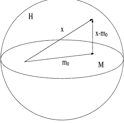
spaces.

Theorem 1 Projection Theorem Let H be

a

Hilbert

space and

M

aclosedsubspace

of H.

Corre

sponding

to

any

vectorx

H,

there

is

a unique vector

mo G

M

suchthat

\\x

-mo||

<

||x

m||

for

all m

G

M.

Furthermore,

a

necessary

and sufficient conditionthat

m G

M be

theunique

minimizing

The Projection Theorem

statesthat

if

we want

to

constructa vector

mo G

M,

a subspace of

H,

thenwe

can

do

so uniquely.

Furthermore,

the

vector

that

best

approximates x will

be

the

one

that

minimizesthe

normof

the

error

vector,

||x

mo

||

,andtheerror

vector,

x mo,will

be

orthogonalto theapproximation

subspace,

M (Figure

2.1)

[22].

Suppose

we want

to

construct anapproximation ofx

G

if from

a set of vectors

y

=

{yi,y2,-,Vn}

G

[image:20.563.154.404.211.459.2]

M,

where

M is

a closed subspace of

H

and

y is

a

basis

of

M.

Then,

the approximation,

or projection

Figure 2. 1

:

Orthonormal

projection

of x onto

M is

a

linear

combination of

j/j

(PMx)

=

Y

aiVi

i=l

(2.8)

where

PM

is

the

projection operatoronto

the

subspace

M [22]. From

the

Projection

Theorem,

the

best

approximation of x will

be

the

one

that

minimizes

\\x

-Pmx\\

and x

-PMx

will

be

orthogonal

to

all

elementsofy,

that

is,

Substituting

(2.8)

into

(2.9)

gives

n

(x-YajyjiVi)=-

(2-10)

Since

the

Hilbert

space

is linear

and

the

inner

product

is

a

linear

operator,

(2.10)

can

be

rewritten as

n

(x,yi)

=

Yaj(yj^i)-c2-11)

If y

G

M is

an orthonormal

basis

of

M,

then

(y,,

yj)

=

0 for i

^

j

and

||yj||

=

1. Equation

(2.11)

reduces

to

(x,yi)

=

ai

(2.12)

making

(2.8)

n

{pMx)

=

Y(xiyi)yi-(2-i3)

2=1

Equation

(2.13)

gives

the

expression

for

the

projectionofthe vector x ontoan orthonormal

basis y

of

M [22].

2.2

Fourier

Analysis

Signal

and

image

analysis

has

long

benefited

from

Fourier

analysis,

where

the

set of

functions,

el2nkx/T,

forms

an orthonormal

basis

of

L2(0,

T),

the

Hilbert

space

consisting

ofall square

integrable

functions

defined

on

the

interval

[0,

T]. All

periodic

functions,

withperiod

T,

alsoreside

in

L2(0,

T),

since

they

can

be completely described

by

one period on

the

interval

[0,

T]. Since

L2(0,

T)

is

a

Hilbert

space,

it

has

an

inner

productandanorm

[10]

defined

as

{f,9)

=

^J^Hx)^x)dx

(2.14)

_ i

11/11

=

{f,f)=(^[\f(x)?dx^

2

(2.15)

Since

ei2nkx/T

is

an orthonormal

basis

of

L2(0,T),

f(x)

G

L2(0,T)

can

be

represented

using

(2.13)

rT

1 fl

ck

=

(f(x),ei2-^)

=

-Jo

f(x)e-^dx.

(2.17)

The

function, /,

is decomposed into

the sum of

infinitely

many

mutually

orthogonal

components,

9k{x)

= Ckel2lTkxlT

, where

orthogonality

means:

(9n,9m}

=

0,

for

_all

m^

n.

(2.18)

That

(2.18)

holds

is

a consequence of

the

fact

that:

wk{x)

=

e?2*kxlT

A;

=

{...,-1,0,1,...}

(2.19)

is

an orthonormal

basis

of

L2(0, T)

[10]. It

is important

to

note

further

that the

orthonormal

basis,

wk,

is formed

by dilating

(known

as

integral

dilation)

a single

function,

ei2nx

Chui

[10]

emphasizes

the

significance of

these

facts in

the

introduction

to

his book:

Let

us summarize

this

remarkable

fact

by

saying

that

every 2-K-periodic

square

integrable

function is

generated

by

a

"superposition

"

of integral

dilations

of

the

basic

function w(x)

= eix.

Chui develops his

section on

Fourier

analysis

assuming

a period of

2tt, thereby

giving

rise

to

his

mention

of

27r

-periodic

functions

and

the

basic function

eix

The decomposition in

(2.16)

and

(2.17)

is known

asthe

Fourier

series expansion of

/(x)[17].

The

basis,

e'27rfex/r,

is

a complex exponentialwith

fundamental

frequency,

o

=

1/71. Integer

_{multiples of}

the

fundamental

frequency

are called

harmonics.

So,

a periodic

function

of period

T,

can

be perfectly

represented

by

the

sum of a complex exponential at a

fundamental

frequency

and

its harmonics.

The

weights of

these

complex exponential

components, ck,

constitute

the

frequency

spectrum of

/.

It is

often

called

the

line

spectrum

because it is discrete.

Square

integrable,

non-periodic,

functions

whose

domain is

the

realnumber

line,

3?,

constitute

the

Hilbert

space,

L2

(3?),

with

its inner

product andnorm

defined

as:

The Fourier

series of

f(x)

G

L2(3)

does

notexist since

/

is

non-periodic and

its domain is

the

entire

real

line,

3. The

frequency

spectrum of

/

can still

be determined

by

taking

its inner

product with

the

function,

el2rr^x,

where

is

thecontinuous

frequency

variable[17].

Letting

uj =

27r

_gives

/oo

f(x)e-^xdx.

(2.22)

-oo

F(u)

is

the

Fourier Transform

of

f(x)

and

is

at

least

piecewise continuous[17].

The Fourier Transform

can

be

interpreted

in

a manner similar

to the

Fourier

series.

A non-periodic,

square

integrable

function,

f(x)

G

L2(3?)

can

be

represented

by

the

integral

sum of complex exponentials with weights given

by

the

frequency

spectrum,

F(w),

1

f

/(*)

=

/

F{u)ewxdu}.

(2.23)

The Fourier Series

and

Fourier Transform

are powerful

tools

for

determining

the

frequency

content

of

discrete

and continuous signals.

However,

in

order

to

study

the spectral

behavior

of

analog

signals

from its

Fourier

Transform,

full

knowledge

of

the

signal

in

the

time

or space

domain

must

be

obtained[10].

In

addition,

if

a signal

is

altered

in

a small neighborhood of sometime

instant,

then

the

entire spectrum

is

affected.

If

a signal of some

frequency

exists

for

a

finite

period of

time,

the

Fourier Transform does

notgive

visibility into

where

in

time the

signal occurred.

Being

able

to

determine

where

in

time

a

sig

nalof some

frequency

occurs

is

called

time

localization.

Being

able

to

determine

the

frequency

content

of a signal at a particular

frequency

is

called

frequency

localization. The Fourier Transform

provides

excellent

frequency

localization,

but

poor

time

localization [10].

In

order

to

obtain

localization in both

time

and

frequency,

an additional parameter must

be

added.

Gabor

[16]

was

the

first

to

adapt

Fourier

analysis

to

include

a modulation

window,

g(x)

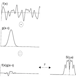
[30]. Gabor's

Short-Time Fourier Transform

(STFT)

[30],

5(r,

u),

is

given as

/oo

f(x)g(x

-r)e~lu}dx.

(2.24)

-oo

The

signal

is

weighted

by

a

finite

duration

window, g(x),

prior

to

taking

the

Fourier Transform (Figure

2.2). The

additional

parameter,

_r,

is

the

translationparameterof

the

window and

it

provides

the

addi

S(yD)

f(x)g(x-t)

[image:24.563.156.409.199.472.2]

<

?

is

present

in

the

signal

for

a

finite

duration,

it

will show

up in

S(t,

u)

at values ofr

corresponding

to

the location

of

the

frequency

pulse.

The

function,

S(t,

u),provides a

two

dimensional

map

of

time

and

frequency

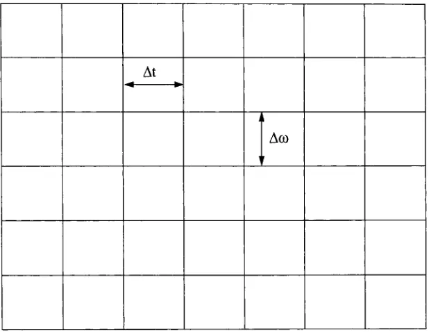
(Figure

2.3)

[30].

By

fixing frequency

at some

value,

u/0>

S(t,

lo0)

gives a

1-D function

indi-At

ii

[image:25.563.128.437.140.379.2]

Am

Figure 2.3:

Time-frequency

map

-

Short Time Fourier Transform

eating

where

in

time

u0

existed.

Alternatively,

by fixing

t = _r0,

S(to,

lj)

gives

the

Fourier Transform

for

that

timeslice of

/.

The

resolution

in

both

timeand

frequency

depend

onthewindow

function

g(t).

Time

and

frequency

resolutionsare

traded

off

according

to the

uncertainty

principle

[10,

30]

1

Time-bandwidth

product =

AtAw

>

where

At

and

Aw

are

the

rms measures of

time

width and

bandwidth

given

by

{J^(s-3(g))|g(s)|2<fr}*

At

=

Au

=

{n.

(W

\\G\\

(2.25)

(2.26)

G(w)

is

the

Fourier Transform

of

g(x)

and

the operator,

E(-)

is

given as

m

-

^}/}fd\

(2.28)

For

this reason,

a gaussian window

is

often used since

it

satisfies

the

equality

of

(2.25)

[30].

However,

modulating

the

signal with a gaussianwindowcorrelates

the

Fourier

coefficients and therefore

destroys

orthonormality.

Furthermore,

the window

function,

g(x),

with

its corresponding

frequency

spectrum,

G(u),

sets

both

the time

and

frequency

resolutions

for

the

entire

time-frequency

plane.

This

is

a

disad

vantage

for analyzing

signals with

both high

and

low

frequencies [10]. In

order

to

properly

represent a

signal of some

fundamental

frequency,

the

window must contain oneor more periodsof

that

signal.

Low

frequency

signals,

therefore,

require

long

time windows,

which corresponds

to

high

resolution

in

the

fre

quency domain. High

frequency

signals require a small

time

window

in

order

to

capture one or more

periods.

The

small

time

windowcorresponds

to

low

resolution

in

the

frequency

domain. The STFT's

windowwidths are

fixed in both

time

and

frequency,

as

illustrated in Figure

2.3,

and

therefore,

cannot

effectively

analyze signals

containing both high

and

low frequencies [10].

The

obvious solution

to

Gabor's Short-Time Fourier Transform is

an orthonormal

basis

of

L2(3?)

that

provides

both

time

and

frequency

localization

for

signalswith

high

and

low frequencies. Wavelet

analysis provides

just

such asolution.

2.3

Wavelet Analysis

The "basic

wavelet"

or

"mother

wavelet"

is

a

function,

ip(x)

G

L2(3R),

whose

Fourier transform,

\1>

(u),

satisfies

the

admissibility

condition

[10, 12, 14, 23,

27]:

C

=

/

l-^pP-du

<

oo.

(2.29)

/

-00 IW

Since tp

(x)

G

L2

(3?),

then

/oo

\Mx)

-oo

|2

must

be

true,

which means

that

ip(x)

must

have,

effectively,

finite

support.

Assuming ^(w)

is

continu

ous,

(2.29)

and

(2.30) imply

*(0)

=0, <?

f

ip{x)dx =

0.

J_oo

(2.31)

This

is

the

reason

that

tp is

calleda"wavelet"

[10]. In

order

for ip

to

have

an averageof

0

(2.31),

it

must

be

wave-like

in

nature.

In

order

for it

to

be in

L2(3R),

it

must

be effectively finite

or of short

duration

as

in

(2.30),

hence

the

term

"small

wave"

or "wavelet."

Equation

(2.31)

also

indicates

that

ip(x) has

the

characteristicsof a

bandpass filter.

If

we

let

, ,_i

, ,x

b.

il>a,b

=

\a\

2V>(^

),

(232)

then the

continuous wavelet

transform

(CWT)

[10, 12,

30]

is defined

as

, r _r

b

Wf(a,b)

=

(/,tM

=

\a\~2

/

f{x)ip{

)dx

(2.33)

J oo ^

where

f(x)

G

L2(?R),

a;

b

G

3?,

anda

^

0. The

parameters,

aand

b,

are

the

scale and shift

parameters,

respectively,

and

they

provide

localization in both

the time

and

frequency

domains. The

parameter

b

centers

the

wavelet at

t

=

b

_andascales

the

wavelet

function,

_ip,on

the

a;-axis.

The CWT is

analogous

to the

Fourier Transform

where

frequency

has

been

replaced

by

scale,

sinceagives

insight into

the

fre

quency

content of a

passband,

not a single

frequency. The bandwidth

of

the

passband changes with a

[10,

30]

suchthat

Aco

=

K.

(2.34)

U!

This

characteristic

is

common

in

communication

theory

and

is

called

"constant

Q"

(Figure

2.4)

[10,

30].

Now,

the

windowing function is effectively

the support ofthe

wavelet,

ip, whichchanges witha.

It

is

not

fixed

as

in

the

case of

the

STFT,

and can

therefore

provide

both

time

and

frequency

localization

of

1

Aa

Ab

Chapter

3

Wavelet

Theory

Development

In

this chapter, the

history

of

the

development

of wavelet

theory

will

be

presented

from

the

original work

of

Morlet

and

Grossman

through the

algorithm

development

of

Stephane Mallat. The development

of

wavelet

theory

wasmotivated

by

theneedtoanalyze a

finite energy

signal with a

single,

finite energy

function,

called a

wavelet,

dilated

andshifted

by

real parameters.

It

wasshownthat

the

conditionon

the

analyzing

function

was simple and

easily

met.

As

the

constraints on

the

dilation

and shift parameters

tightened,

for

instance,

confinement

to

%>,

the

conditions on

the

analyzing function

also

increased. It

was shown

by

Meyer

that

if

the

dilation

parameter values were constrained

to

be

powers of

2

and

the

shiftparametervalues

to

be integer

multiples ofpowersof

2,

then awavelet could

be found

such

that

its

shifts and

dilates formed

anorthonormal

basis

of

L2(K). This

chaptergoes

through

in

chronological

order

the

development

of each"class"of wavelet and

the

conditions associated with

each,

culminating

with orthonormal

bases

and multiresolutionanalyses.

3.1

Continuous

Wavelet Transform

J.

Morlet,

a

French

geophysicist,

first

proposed

the

use of

"wavelets

of constant

shape"

for

analyzing

seismic

data. His

reference

to

constant shape was

intended

to

contrast thesenew

functions

with

the

Short Time Fourier Transform

(STFT),

which are not ofconstantshape

[14].

A.

Grossman,

a

French

a square

integrable

representationof

functions

in

I/2(3ft)

and

this

representation was referred

to

as

the

wavelet

transform

[14,

30]. The

wavelet

transform

is defined

as

follows:

Definition 3

(Continuous Wavelet

Transform)

[10]Ifip

G

L2(3)

satisfiesthe "admissibility" con

dition:

_

[ |*(w)|2

C,/>

=

/

| |

doj

< oo,

(3.1)

J-oo

|w|

wften?

*(w)

wr/ze

Fourier

transform oftp,

then

ip is

called a

"basic

wavelet".

Relative

to

every

basic

wavelet_{ip, the}continuous wavelet

transform

(CWT)

on

L2(3?)

is

defined

by

Wf(a,b)

=

(f,ipa,b)

f

i

(

x

-b\

=

J^f(x)\a\-21p\jdx

(3.2)

for

f

G

L2(3?),

and

a,

b

G

3?

witha

^

0.

The

wavelet

operator,

ipa,b(x)

=

\a\-*ip

(^

J

,

(3-3)

is

a

dilated

and shifted version of a single

function,

ip(x),

sometimes referred

to

as

the

mother

wavelet,

and

it

maps a one

dimensional

signal

into

a

two

dimensional

analysis

domain,

that

is,

scale,

a,and

shift,

b. This mapping

provides

visibility into

the

frequency

contentof asignalthrough

the

scale

parameter,

a,

and

time

localization

through the

shift

parameter,

b,

a significant advantage over standard

Fourier

analysis.

Figure3.1

shows

the

effect of

the

dilation

and shift

parameters,

aand

b

on

the

wavelet operator.

The

wavelet

shown,

used

by

Morlet

andGrossman,

is

acosine

function

modulated

by

agaussianwindow.

Notice

that

as a

increases,

the

wavelet gets wider and shorter

in

height

and when a

decreases,

the

wavelet

gets

thinner

and

taller.

This

effect provides a

zoom-in,

zoom-out

capability in

the

frequency

domain.

The bandwidth

of

the

wavelet

for

small a

is

large

and

the

bandwidth for large

a

is

small.

Of

course,

changes

in b

shift

the

wavelet

up

and

down

the

x-axis

giving

full

two

dimensional latitude

in

both

time

and

frequency.

The

admissibility

condition

(3.1)

on

ip

implies

T f

*(0)

=0 <=>

/

ip(x)dx =

0.

(3.4)

a=2

b=-2

\t=-a=0.5

b=1

a=0.25

b=3

Figure 3.1:

The Gabor

or

Morlet

wavelet

Therefore,

tp

has

an average value of

0,

acts

like

a

highpass

or

bandpass filter

and

hence

must oscillate.

The

fact

that

ip

G

L2(3)

means

that

ip has finite energy

and

therefore

must

fall

off

fairly

rapidly.

These

two

features

are what motivated

Morlet

and

Grossman

to

refer

to these

functions

as"wavelets"or short

waves.

The admissibility

condition

(3.1)

was not

specifically derived

with

these

features in

mind.

Rather,

the

admissibility

condition

is

necessary for

the

inverse

transform to

exist and

for

the

inverse

wavelet

operator

itself

to

be

a shifted and

dilated

version ofa mother

wavelet,

referred

to

as

the

dual

of ip.

Theorem 2 (Inverse Wavelet

Transform)

[10]

Let ip be

a

basic

wavelet which

defines

a

CWT,

Wf.

Then

i /-oo /-oo

dadb

f(x)

=

7T

/

W7MWa,6(s)-2-(3-5)

(sip

Joo

Joo

"

D

Kaiser

[19]

providesa

very

understandable

derivation

of

both

the

Inverse Wavelet

Transform

and

the

for dyadic

waveletsand

frames.

Using

Parseval's

theorem,

(3.2)

can

be

rewritten as

Wf(a,b)

=

(f,i,aJb)

=

(F^a>b)

(3.6)

where

F()

is

the

Fourier Transform

of

f(x)

and

*a,6(0

is

tne

Fourier Transform

of

ipa,b{x),

given as

*a,ft(0

=

\a\h-i2*tb*{a)

(3.7)

where

\&()

is

the

Fourier Transform

ofip(x).

Expanding

the

inner

product of

(3.6)

gives

/oo J

Wf{a,b)

=

/

F{)\a\2y{a()e-i2^bd

Joo

-oo roo , /-oo =

\a\2

/

F()*K2^6d

(3.8)

JOO

The

right

side of

(3.8)

is

the

Inverse Fourier Transform

of

F()\I>(a),

so

taking

the

Fourier Transform

of

both

sides with respect

to

b

gives

/oo ,

Wf{a,b)e-l2^bdb=

|o|2F()tf(a)

(3.9)

-oo

Kaiser

uses some clever manipulation

to

isolate

F()

in

(3.9).

He

multiplies

both

sides

by

|o|

2

\JJ(a)

and

integrates

with respect

to

awhere

the

measureof

integration

is

da/\a\2

rr^.,wiM,-*^

=

r>oi(.oi

Joo Joo

|"|

Joo

|0|

=

f-(

/

I*(a0|2n

./-oo

|a|

=

TOZtf)

(3.10)

where

stf)

= /

l*K)l2n-

(311)

Joo

\\

Choosing

da/|a|2as

the

measureassociatedwith

the

integral

in

(3.10)

guarantees

that

the

admissibility

condition

is

aconstantand

therefore

guarantees

that the

dual

can

be

representedas a shifted and

dilated

version ofamotherwavelet

[19]. Now

F()

in

(3.10)

can

be

solved

if

and

only if

0

<

A

<

Z~l

()

<

B

<

00,

F(0

=

Z~\i)

r

r

W7M)|a|*(a0e-**^.

(3-12)

Substituting

w =

at;

in (3. 1

1)

gives

the

admissibility

condition,

which

is

a constant and

therefore

bounded,

|*(w)12

-dto

(3.13)

-oo

|<^|

Substituting Z()

=

C,/,

in

(3.12)

_and

taking

the

Inverse Fourier Transform

of

both

sides with respect

to

gives

1

foo foo

___ . i

/x-b\ dndb

(3.14)

f{x)

=

yr

/

W7(a,6)a

^V

y-(^

./-ooy-oo

V

a /

|a

x

-b\

dadb

which

is

the

form

of

the

Inverse Wavelet Transform

given

in Theorem 2.

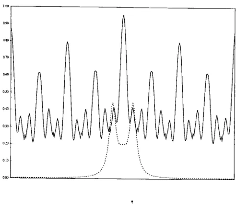
Figure 3.2

shows an exampleofa continuous wavelet

transform.

The

signal

being

analyzed

is

a

tran

sient sinusoidwith

exponentially

decaying

amplitude.

The analyzing

wavelet

is Morlet's

wavelet

from

Figure 3.1. The

horizontal

axis

is

shift,

b,

and

the

vertical axis

is

scale,

a with a

increasing

downward.

Hi

Figure

3.2:

Continuous Wavelet Transform

of atransientsignal

The

transient

signal

has

an average value of

0,

so

for large

valuesof

a, the

CWT

vanishes since a

very

wide wavelet

tends to

average over

the transient

signal.

The CWT

alsovanishes

for

very

small values of a since

the

signal appears constant over a

very

short

interval.

There

is

a value of

a,

however,

that

coin cides

very nicely

with

the

oscillation of

the transient signal,

thereby

producing

a

very

large

response

in

the

shift

parameter,

b,

givestheapproximate

location

of

the transient

signal.

The

continuouswavelet

transform,

characterized

by

a,

b

G

3?,

wherea

^

0,

is

rathersimple

to

use

and requires

very few

restrictions on

the

analyzing

wavelet.

However,

it

contains a

lot

of

redundancy

and

is

computationally intensive.

Notice in Figure 3.2

the

high

degree

of correlation

in

the

CWT. This

cor

relation

is

due

to the

redundancy

andcan

be

removed

by

less

redundant representations.

The

following

sections willshow

the

development

of

different

classes of wavelets with

lesser degrees

of

redundancy

asa and

b

are

further

constrained.

While

theseconstraints add conditions on

the wavelets,

they

lead

to

the

generation of

bases,

new

design

techniques,

and

fast

algorithms

for

the

wavelet

transform.

3.2

Dyadic Wavelets

In

order

to

reduce

the

computational

burden

of

the

CWT,

let

the

scale parameter

take

on values of a =

V

where

j^

and

b

G

3ft. The

wavelettransform

becomes

Wf{2>,b)

=

(f,ip2J<b)

/oo ,

=

/

f(x)

2-2ip(2'Jx-bTd)dx

(3.15)

Joo

This

class of wavelets

is

known

as

"dyadic"

waveletsand are

defined

as

follows:

Definition 4 (Dyadic

Wavelets) [10]

A function ip

G

L2(3ft)

is

called a

dyadic

wavelet

if

there exist

twopositive constants

A

and

B,

with

0

<

A

<

B

<

oo, suchthat

2

<

B.

(3.16)

A<

Y

|*(2~J'w)

j=-oo

Condition

(3.16)

is known

as

the

stability

condition and again

is driven

by

the

necessity for

an

inverse

transform.

Since

(3.15)

has

the

same

form

as

the

CWT,

but

with a =

2J,

then

(3.11)

must still

hold

where a=

2j.

Substituting

Aa

= 2^+1 - 2j ₌ 2j

for

da

gives

da/

a=

1.

Summing

over

j

gives

z(0

=

Y\v{2Jz)\2

(3-17>

jEZ

As

before,

Z()

must

be

bounded,

which

leads

to the

stability

condition

0

<

A

<

Y

|*

(2J0

jez

Notice

this time that

Z()

mustnot

necessarily be

a constant.

However,

since

it is

bounded,

the

Inverse

Wavelet

Transform

can

be found

by

substituting

a = 2J and

Aa

= 2J

into

(3.12)

and

summing

over

j

instead

of

integrating

over_a,

F(0

=

Y

r

Z-\i)Wf{2\b)2^{2^)e-i2^b~

jeZJ-oo L> =

Y

[ 2~JWf(2j,b)22ty{2J0e-i2ntb

(3.19)

jez

J-2J

where

*(f)

=

#(f)/Z(f)

and

Z{()

is

given

in (3.17).

Taking

the

Inverse Fourier Transform

of

both

sides of

(3.19)

gives

the

expression

for

the

Inverse Wavelet Transform using dyadic

wavelets,

/(*)

=

Y

I"

2~JWf(2?,b)2-H

(X^)

db

(3.20)

jeZJ-oo

\

lJ

J

where

ip(x) is

the

Inverse Fourier Transform

of

Sfr()

and

is

the

dual

wavelet

to

ip(x).

3.3

Frames

The

next

step in reducing

the

computational

burden

of

the

CWT

is

to

sample

the

shift

parameter,

letting

bj^k

=

k2^ba,

_where

bo

is

_{a constant}

known

_as

the

sampling

rate

[10]. Now

the

wavelet operator

is

given

as

iPbo-j,k(x)

=

2-2iP(2-iX

-kb0)

(3.21)

and

the

wavelet

transform

given

by

W/(ai,6J-fc)

=

(/,^6oW-,fc)

(3.22)

The

condition on

the

waveletalso

tightens

beyond

the

stability

condition,

namely,

^||/||2<

Y

K/^o;i,*>|2<|l/U2

(3-23)

j,kez

where

||

||2

is

the

L2(3ft)

norm and

0

<

A

<

B

<

oo.

This

condition

is identical

to that

for

a

frame

of

L2

(Jr.)

,

meaning

that

in

order

for ip

to

be

a wavelet with

the

statedconditionson a and

b,

it

mustgenerate

Definition

5 (Frames

of

L2(U)) [10]

A

function ip

G

L2(3ft)

is

saidtogenerate a

frame

{ipb0-,j,k}

of

L2(3ft)

with

sampling

rate

bo

>

0

if

(3.23)

holds for

some positive constants

A

and

B,

whichare called

frame bounds.

If

A

=

B,

_{then the}

frame is

_calledatight

frame.

Before giving

the

expression

for

the

inverse

transform,

let T be

a

linear

operatoron

I/2(3ft),

defined

by

Tf=Y

(f^b0;jtk)A0;j,k

(3.24)

j,kez

where

/

G

L2(3ft). Then

the

dual

of

ipb0-,j,k

is

given

by

ip{f

=

T~lipbo]jtk

_and

the

inverse

_wavelet

transform

by

j,kez

If

A

=

B

=

1,

then ipb0;j,k

is

_{an orthonormal}

basis

_of

L2(3ft). If A

=

B

^

1,

then the

frame

is

called

a

tight

frame,

which acts

like

anorthonormal

basis,

but may

not even

be

linearly

independent

[12].

The

intent

of

discretizing

both

the

scaleandshift parameters

is

to

reduce

the

redundancy

ofthewavelet

trans

form. Frames

provide an

intermediate step between

the

continuous wavelet

transform,

which contains

the

maximum amount of

redundancy,

andwaveletorthonormal

bases,

whichgenerate

decompositions

with no redundancy.

The

ratio of

the

frame

bounds, B/A,

acts

like

a

redundancy indicator. For

instance,

in

speech

processing,

B/A is

very

large

indicating

a

lot

of

redundancy in

the

wavelet

transform

and

in

fact

approximates

the

continuous wavelet

transform

[12].

At

the

other

extreme,

applications

like image

compression,

requiring

no

redundancy,

constrainthe waveletsso

that

they

generate a

tight

frame,

that

is,

B/A

=

1.

A. Grossman

with

the

help

of

Y. Meyer first

realized

the

importance

of

the

frame

concept with re

gards

to

wavelet analysis.

Meyer

showed

how

the

wavelet

frame

construction was

the

sameas

that

of

the

Weyl-Heisenberg

coherent states.

However,

for

the

W-H

coherent

states,

if

a

basis,

g,

was required

(no

redundancy)

as opposedtoa

frame,

theneither

xg(x)

or

wG(w)

wasnotsquare

integrable (not in

L2(3?))[12]. Meyer

set out

to

show

that

Grossman's

wavelet

frames

were subject

to the

same

limitation,

but instead

discovered

a

bandlimited,

orthonormal wavelet

basis

such

that

xip(x)

and

w$(w)

were

both

in

L2(!ft)

[13].

This

discovery

led many

ofthewavelet pioneers

toward

developing

themathematics

for

3.4

Orthonormal Wavelets

Y. Meyer

showed

that

for

a

- _2j

and

b

= k2i

(assume

b0

=

1),

there

exists a

family

of

functions,

{V'j.jfe

=

2~:>/2ip(2-3x

-k)}

that

form

anorthonormal

basis

of

L2(K).

Chui

and

Mallat define

anor

thonormal

wavelet

basis

as

follows.

Definition 6

(Orthonormal Wavelet

Bases)

[10, 23,

27]

A function ip

G

L2(3?)

is

called an orthonor

mal wavelet

if

the

family

{ipj,k},

is

anorthonormal

basis

ofL2(?R), that

is,

(i>j,k, i>l,m)

=

Sj,i h,m

(3.26)

where

Sj,k

= '

1

for

j

=

k

0

j^k

(3.27)

and

every

f

G

L

(3?)

can

be

written as

00 oo

/(*)=

Y

Y

d{2L2iP{2jx-k)

(3.28)

j=ook= oo

Equation

(3.26)

indicates

that the

family

of

wavelets, ipjtk

is

orthogonal

in

two

dimensions. Integer

translates

of

the

wavelet at a given scale are orthogonal

to

one another

(6k^m)

as are wavelets at

two

different

scales

(5jj). At

a given

scale,

j,

(ipj)k,ipj,m)

=

5k,m

_and

ipjjk

forms

an orthonormal

basis

of

Wj,

a subspace of

L2(3). Because

of

orthogonality

across

scales,

Wj

J.

Wj

for

all

j

^

I.

Therefore,

applying (2. 1

3)

to the

projection of

/

onto

Wj

gives

oo

9i(x)

=

(Qi,f)(x)=

Y

d{2L2iP(Vx-k)

(3.29)

k oo

where

gi(x)

G

Wj

and

/oo

4

=

</. Vv,fc>

=

/

f{x)22iP{Vx

-

k)dx

(3.30)

J

oo

Qi

is

the

projectionoperator withrespect

to the

basis

ip.

Substituting (3.29)

into

(3.28)

gives

oo

which says

that

/

can

be decomposed into

an

infinite

sum of

its

projections ontoorthogonal _subspaces,

Wj

[10].

Furthermore,

L2(5ft)

can

be

expressed as

the

direct

sumoforthogonal subspaces

Wj

L2(3ft0

=

...+W_1+Wo+Wi+...

(3.32)

Because

the

wavelet

has

the

characteristic of a

bandpass filter

(3.4),

the

projection

operator,

Q3,,

is

effectively projecting

or

filtering

out

the

detail

or

high

frequency

content of

/

at scale

j,

and

(3.31)

shows

that

/

consists of

the

infinite

sum of

these

detail

functions,

(QLf){x)

[10, 12, 23,

27].

Furthermore,

the

detail

functions

{Q^f){x),

contained

in

Wj,

are orthogonal

to

oneanother since

Wj

_L

W\

for

all

j

^

I.

3.5

Multiresolution Analysis

A

major

breakthrough in

the

understanding

of orthonormalwavelet

bases

came when

Y. Meyer

and

S.

Mallat

imposed

the

concept of multiresolution analysis on wavelet

decompositions [14].

Mallat

had

been working

with

the

Laplacian

pyramid algorithm

developed

by

Burt

and

Adelson

[6]

and recognized

that thesequence of

functions

generated

by

an orthonormalwaveletwere

in

essence"detail"

functions

that

representated

the

information lost in going from

onescale

to

a

lower

scale

[13].

He

and

Y Meyer

developed

the

mathematics

for

what came

to

be known

as amultiresolution analysis.

Let

Vj

be defined

as a subspaceofL2

(5ft)

where

Vj

=

...

+Wi_3+Wj_2+Wi_1

(3.33)

Then,

the

direct

sum

decomposition

of

L2(5ft)

in

(3.32)

can

be

rewritten

[10, 23]

as

L2(3fJ)

=

Vj+Wj+Wj+i+

(3.34)

From

(3.33),

it is

clear

that

Vj+1

=

Vj+Wj

(3.35)

and

Vj

forms

a nestedsequenceof subspaces of

Z/2(Jft),

that

is,

Let

<pjtk

be

a set of

functions

thatspansthesubspace

Vj

[10],

where

(pjtk

= 2%

4>(2jx

-k)

(3.37)

Then,

any function in

Vj

can

be

represented

by

a

linear

combination of</>jjfe.

oo

P(x)=

Y

&*<P@x-k)

(3.38)

k=_oo

Assume

4>jtk

forms

an orthonormal

basis

of

Vj,

then

((f>j,k,(f>j,m)

=

h,m

(3.39)

and,

4

=

</j(*)A*>

(3-40)

This

assumption

is

not as

bold

as

it may

seem.

The Fourier

transform

of

(3.39),

called

the

Poisson

sum

mation,

is

a

27r

periodic

function

given

by

00

Y

|$(w

+

27rfc)|2 =

1

(3.41)

k=_oo

where

3>(w)

is

the

Fourier

transform

of <p{x).

Let0(x)

be

a

function

such

that

(^

spans

V}, then^>j_(x)

can

be found

such

that

it

satisfies

(3.39)

by

way

of

the

following

orthogonalizing

"trick"and

taking

the

inverse Fourier

transform

[10]:

*M

=

^

r

(3.42)

(Er=-ool^

+

2^)|2)

=

where

0

<

A

<

| EfeL-oo

l$(w

+

2nk)\2

<

B

<

oo

for

allu.

Because

a non-orthogonal

function

that

spans

Vj

can

be

orthogonalized

using

(3.42),

it is

safe

to

assume

that (pj>k

is

orthonormal

in

the

first

place.

Now,

if

fj

is

_a

function in

the

_subspace

Vj,

then

by

(3.35)

it

can

be

represented

by

the

sum of

its

projections on

Wj_i

and

V}_i

[10,

12]

f(X)

=

Since

Q^,-1(/)

represents

the

detail

off3 at scale

j

1,

then

7^_1(/)

must represent fJ with

those

details

removed,

that

is,

a

lower

resolutionapproximation offJ at scale

j

-1

[10,

12,

23]. Subsequent

projectionsonto complement

subspaces,

V

and

W,

produce

the

decomposition map

shown

in Figure 3.3.

Vj

contains

lower

and

lower

resolution approximations of f3 as

j

- -oo.

The

nested sequence of

V=U(W)

Vi

"j-2

'j-i

Wj,

'Wj.2

Vj-3

Wj.3

Figure 3.3:

Multiresolution Decomposition

of

L2(3f)

subspaces

is

called a multiresolution analysis and satisfies

the

following

conditions:

Definition 7 Multiresolution

Analysis/70, 12, 23,

24,

27]

The

sequence

of

subspaces,

Vj,

form

a multiresolution analysis

if

the

following

conditions aresatisfied:

1.

...cV-iCVoCVi...;

2.

closL2

({JjeZVj)

=

L2(5ft);

3-

f)jZVj

=

{0};

4.

Vj+i

=

5.

f(x)eVj^f{2x)Vj+ujeZ

Items 7.1

and

7.2

state thata multiresolution analysis

is

anested sequenceofsubspaces whose union

spans

L2(5ft). Item 7.3

states

that

there

is

no portionof

L2(3?)

that

is

common

to

all subspaces

Vj,

except

the

all zero

fun