Portable high speed data acquisition system for ultrasound tissue characterization

1-1-1992

Portable high speed data acquisition system for

ultrasound tissue characterization

Vincent J. Doerr

Iowa State University

Follow this and additional works at:https://lib.dr.iastate.edu/rtd

This Thesis is brought to you for free and open access by the Iowa State University Capstones, Theses and Dissertations at Iowa State University Digital Repository. It has been accepted for inclusion in Retrospective Theses and Dissertations by an authorized administrator of Iowa State University Digital Repository. For more information, please [email protected].

Recommended Citation

Doerr, Vincent J., "Portable high speed data acquisition system for ultrasound tissue characterization" (1992).Retrospective Theses and Dissertations. 18117.

•) _,

by

Vincent J. Doerr A Thesis submitted to the

Graduate Faculty in Partial Fulfillment of the Requirement for the Degree of

MASTER OF SCIENCE

Interdepartmental Program: Biomedical Engineering

Department: Electrical Engineering and Computer Engineering Co-majors: Biomedical Engineering

Electrical Engineering

Signatures have been redacted for privacy Signatures have been redacted for privacy

Iowa State University Ames, Iowa

TABLE OF CONTENTS

CHAPTER 1. INTRODUCTION

Ultrasound Background Beef Grading Background

Ultrasound Beef Grading Background Statement of Purpose

CHAPTER 2. MATERIALS AND METHODS System Design

Data Acquisition Board Hardware Description Microcontroller Software Description

PC System

Carcass Data Collection Methods

CHAPTER 3 RESULTS AND DISCUSSION System Results

Impulse Response

Time Gain Control Results Filter Results

Power Requirements Cost Requirements System Limitations Data Analysis

ACKNOWLEDGMENT 37

APPENDIX A DATA ACQUISffiON BOARD SCHEMATIC

DIAGRAM 38

APPENDIX B. MICROCONTROLLER ASSEMBLY LANGUAGE

SOURCE CODE 40

APPENDIX C. MICROSOFT QUICK BASIC SOURCE CODE 47

APPENDIX D. DATA PROCESSING ALGORITHMS 56

APPENDIX E. DATA ACQUISffiON BOARD BILL OF

LIST OF FIGURES

Page

Figure 1.1 Chart used to determine carcass grade from the assigned

marbling score (USDA, 1965) 4

Figure 1.2 Visible marbling used by USDA Graders to determine the

marbling score (Anselmo et al., 1987) 5

Figure 2.1 Complete Data Acquisition System 7

Figure 2.2 DAB block diagram 9

Figure 2.3 Pulser waveform at turnoff time (X-axis 5 usec/div): CHl

(top trace) MOSFET gate voltage (5 V / div), CH2 (lower

trace) voltage spike across the transducer (5 V /div) 10

Figure 2.4 Time gain control compensation for a 2 MHz sine wave

over 25.6 microseconds. The gain increased from 23 dB

to 33 dB over this time period 12

Figure 2.5 Microcontroller software flow diagram 15

Figure 2.6 Demonstration of TGC ramp shifting (CHl: Acquire signal

2 V /div, CH2: TGC ramp, 0.5 V /div, X-axis is lOusec/div): A) data acquisition starts at a low gain, b) data acquisition

starts at a high gain 18

Figure 2.7 Pulser timer outputs and amplifier enable output (CHl:

amp enable, 2 V /div, CH2: pulser timer, 2V / div, X-axis:

5 usec/div) 19

Figure 2.8 Microcontroller timer outputs: pulser (top signal),

amplifier enable (second signal), Acquire (third signal), and TGC (bottom signal): X-axis 20 usec/ div. All signals

are 0 to 5 V (6 V / div) 19

Figure 3.2 Frequency domain impulse response (1 MHz/div, arbitrary

amplitude) 24

Figure 3.3 Demonstration of TGC effectiveness (X-axis 5 usec/ div,

amplitude 1 V /div at DAC): a) Ultrasound reflection from meat sample with TGC, b) Ultrasound reflection from the

same meat sample without gain compensation 25

Figure 3.4 Bode plot generated using a constant magnitude sine wave

input (X-axis: frequency in Hz, Y-axis: amplitude in dB

with 5 dB/ div scale) 26

Figure 3.5 A-mode ultrasound reflections viewed from the dorsal

side of the longissimus dorsi from 2 cm depth to 5.8 cm: a) sample with marbling score of moderately abundant

60%, b) sample with marbling score of slight 50% 29

Figure 3.6 Spectrum of reflected signals (X-axis: 2 MHz/ div, Y-axis

relative amplitude): a) before filtering, b) after 5-point

moving average filter ₃₀

Figure 3.7 Marbling score verses -12dB bandlimits (Y-axis is

frequency in kHz): a) high frequency bandlirnit, b) low

frequency bandlirnit ₃₂

Figure 3.8 Marbling score verses peak frequency (Y-axis is

Table 3.1

LIST OF TABLES

Marbling score, spectral peak frequency, -12 dB bandlimits, and -12 dB bandwidth for 21 carcass samples

Page

This research involves the design and testing of an application specific portable ultrasound data collection system which can be used to discriminate between levels of intramuscular fat (marbling) in beef tissue. First, pertinent background information is reviewed, and the need for such a system is justified.

Ultrasound Background

Sound energy in the frequencies above the audible range is classified as ultrasound. There are a number of scientific and medical uses for ultrasound, including material fault detection and imaging. For imaging, pulse mode ultrasound is used. A burst of sound energy is sent out by an ultrasound transmitter, and an ultrasound receiver (often the same transducer) listens for echoes. The time delay between sending and receiving the signal, along with the velocity of sound for the medium, are used to calculate the distance between boundaries which caused reflections. Methods of using the reflections to produce an image include amplitude mode (A-mode), and brightness mode (B-mode) (Webster, 1978). A-mode imaging detects boundaries by applying a threshold function to the reflected signal. B-mode imaging produces a two-dimensional image by using a linear array of A-mode transducers. By applying a number of thresholds, a gray scale image can be produced.

In addition to imaging, pulse mode ultrasound has been used to characterize

A boundary is any discontinuity where the media on either side of the discontinuity have different acoustic properties (specifically, acoustic impedance). The amount of the signal reflected and transmitted at a planar surface interface can

be determined by the following equations (Wells, 1969 pp 11-12):

Pr/Pi= (Z2 cos a- Z1cos b) / (Z2 cos a +Z1 cos b) Pt/Pi = (2 Z2 cos a) / (Z2 cos a + Z1 cos b)

where Pr/ Pi is the pressure reflectivity of the interface

Pt/ Pi is the pressure transmissivity of the interface Z1 is the acoustic impedance of medium 1

Z2 is the acoustic impedance of medium 2

a is the angle of incidence of the wave b is the angle of refraction of the wave

The acoustic impedance of muscle tissue is 1.70 x 10-5 (g / cm2 sec), while it is 1.38 x 10-S for fat tissue. Therefore, the power reflected at an ideal planar boundary

of muscle and fat with normal incidence would be approximately 1 % of the incident

power (Wells, 1969, pp8-13).

the distance traveled.

The attenuation of soft tissue (for example, muscle or fat) is often approximated (Wells, 1969) to be 1 decibel per centimeter of tissue per megahertz (dB/cm/MHz), where the MHz term is the frequency of the sound.

Beef Grading Background

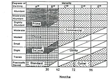
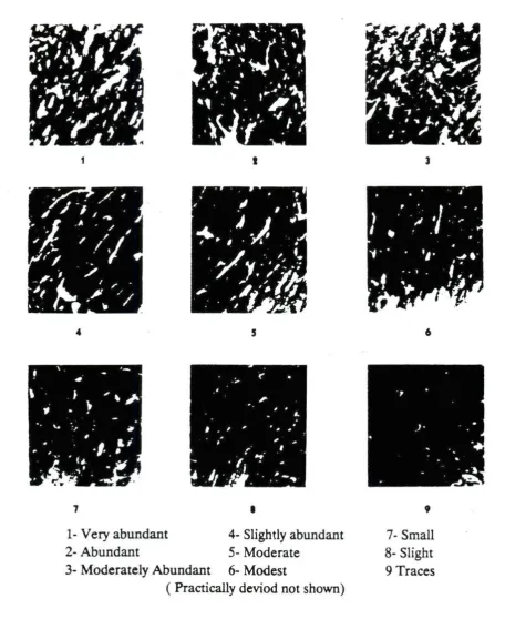
Beef coming from young cattle is classified at the time of slaughter as one of four quality grades including prime, choice, select, and standard. Figure 1.1 shows the USDA chart which is used to correlate the level of marbling of a beef carcass with the grade assigned to that carcass (USDA, 1965). The marbling score is determined by a subjective evaluation of the intramuscular fat of the longissimus dorsi muscle at the quartering point of the carcass between the 12th and 13th rib. This evaluation is done by trained USDA meat inspectors after the carcass has been cooled. Figure 1.2 shows pictures of the visible marbling used for comparison between the marbling score (Anselmo et al., 1987).

Ultrasound Beef Grading Background

[image:11.573.95.469.103.385.2]

Figure 1.1

Oe9rees ol

Marblin9 _{A'° 8'°}

c10

o~

'"''

Abundanl _!t:

. ~.

[I

Mod•rately 'r.

Abundant , ... .•.·•·.·•·.·. -:·:·.·.·.·.· •.·.·.·.:·.·.·

Slo9/Hly _~Prime

Abundant

.

.

.

.

. .

.

.

. .

.

. . .

... .

.·.·.·.·.··:· ·:·.·.·.·.·.· ·.·•··.·.·.·•·

...

-

...

"'

..

···.·

.·

...

:~··

Moder 1 t e1-~f:1f:t:'.· j::j::j::~1t:t:~t:~t:~~~~

. ·• • •

Comm ere i al • •. •. • • •

I • • • e e e e e l • • • e • •. • • e

C"' . ~~ ...

--r· ...

-~~ ~

Modest ,..,_,.. 1101ce •••• •. •••• • ••

I J I I • • • • e e

Small H-1-+-':'-H'-t-t'-t-t-t'~-t-t"':i~_{I"- I I I I T} ~-...

. .

•

Traces

Practically f+ Standard , 1 r.J v

Devoid rt 1 ' • • 1. L l • ,.., '"Y"" ~--.·.-.··~ ~

..

·.

:Cutt;;·:~.-·.-:_~

• ...

:ti~

30 42 72 96

Mouths

Chart used to determine carcass grade from the assigned marbling score (USDA, 1965)

.

r,

·''

~,~I'

_{1'1,• .}

..

_{' .}

.

·~

·"

.

,,-.,

,

.

..

..

. • _·., J

it·

I

·,,i .. '

'-·I~

·

,

·'1

..

...

. /

. I

_,

..

_/'

f

t

s

(' .,.

.

_,.

,

.

L

'

. ,

_, , I

.

..

f . ~ ..

,

..

.

,

..

--

~

7

•

1- Very abundant 4- Slightly abundant

2- Abundant 5- Moderate

3- Moderately Abundant 6- Modest

(Practically dcviod not shown)

J

i

)

I

-r

""

' .

.'

J

_...

-

.

'1 .•

.,.

_,f

~..,.

.

.

.

I

6 9 7- Small 8- Slight 9 Traces .it· '

.

I~ I

[image:12.574.55.512.53.612.2]

/ ·

Figure 1.2 Visible marbling used by USDA Graders to determine the marbling

Whittaker et al. (1990) showed that a combination of spectral components (including center frequency, bandwidth, and spectral shift) of reflected ultrasound signals could be correlated with marbling score. Woods and Miles (1986) demonstrated a correlation between muscle concentration in beef tissue and

attenuation and velocity of ultrasound. Haumschild and Carlson (1983)

demonstrated that Bragg scattering could be used to correlate the beef grades in

isolated samples of tissue extracted from the longissimus dorsi. Amin (1989) and

Widyaatmadja (1991) demonstrated that attenuation measurements could be used to correlate with the fat content of longissimus dorsi samples. Chang (1991) demonstrated that reflected energy and spectral shift could be correlated with fat content in longissimus dorsi samples.

The above studies were performed on isolated meat samples in a laboratory

setting with a large amount of laboratory equipment. If these techniques are to be

applied in a beef grading system, a portable ultrasound data acquisition system is needed.

Statement of Purpose

CHAPTER 2. MATERIAL AND METHODS

A portable ultrasound data acquisition system for tissue characterization was designed and implemented. This system was used to acquire raw ultrasound data from beef carcasses within an hour of slaughter. These ultrasound signals were analyzed to discriminate between levels of intramuscular fat.

System Design

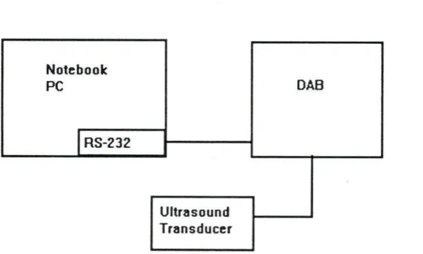
A microcontroller based high speed ultrasound data acquisition circuit board (DAB) was designed and built. This board was designed to communicate with a portable personal computer (PC). The communication involved down-loading commands from the PC to the DAB and up-loading a digitized ultrasound signal from the DAB to the PC. Figure 2.1 shows a block diagram of the resulting system.

Notebook

PC DAB

I

RS-232

[image:14.572.137.445.434.619.2]

Ultrasound Transducer

Data Acwiisition Board Hardware Description

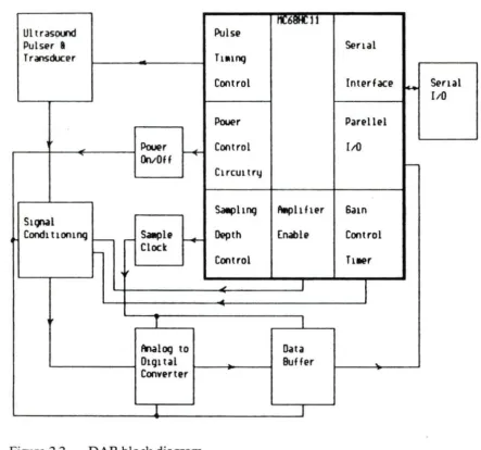
Figure 2.2 shows a block diagram of the DAB (see Appendix A for a complete schematic diagram of the DAB). The circuit consists of an ultrasound pulser, an ultrasound transducer, analog signal conditioning circuitry, a flash analog to digital converter (ADC), a high speed data buffer, a serial interface, and power supplies. The circuit also includes an embedded microcontroller which coordinates the actions of all the other circuits.

The ultrasound transducer and pulser The ultrasound transducer used in this

system is an inductively tuned PZT transducer manufactured by Renco1 _(serial

number 3701), with a center frequency of 2.2 MHz. This transducer was used as a burst mode transmitter and as an echo receiver. For pulsing the transducer, a

P-channel MOSFET (Ql) is used as a switch in series between a voltage source ( + 9

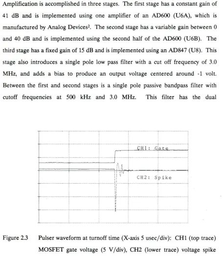
V) and a diode (Dl) which connects to the transducer (Trl). While the switch is closed, current flows through the tuning inductor of the transducer. When the switch is opened, the energy stored in the magnetic field of the inductor causes a large voltage spike across the piezoelectric transducer which then emits a burst of sound. Figure 2.3 shows the gate voltage of the FET at turn off time as well as the resulting voltage spike at the transducer. The MOSFET is driven by a decoder (74HC138) with a zener diode used for level shifting. The decoder is driven by the microcontroller.

rw.;6tn: l 1

Ultrasound Pulse

Pulser

a

Serial

Transducer

_-

Tl•tnq

Control lnterf.1C:e _IC.+ Serial

1/0

Pouer Parellel

~ Pouer

--+ Control 1/0

OrvOff

-Circu1 try

Sallphnq ti.ph her Sain

StQNl

, ~ Conch tt om nq

-

_.- ~le

,_...

Depth [n.lble Control

-

Clock

Control Tl.er

~

, I I

I

~

~ T I

Analog to Oat~

01g1 ul ~ Buffer ~

Converter

[image:16.573.55.498.112.526.2]

1 I

Figure 2.2 DAB block diagram

Si~al Conditionini Circuitzy The signal conditioning circuitry is designed to

Amplification is accomplished in three stages. The first stage has a constant gain of

41 dB and is implemented using one amplifier of an AD600 (U6A), which is

manufactured by Analog Devices2• The second stage has a variable gain between 0

and 40 dB and is implemented using the second half of the AD600 (U6B). The

third stage bas a fixed gain of 15 dB and is implemented using an AD847 (US). This

stage also introduces a single pole low pass filter with a cut off frequency of 3.0

MHz, and adds a bias to produce an output voltage centered around -1 volt.

Between the first and second stages is a single pole passive bandpass filter with

[image:17.570.58.516.85.609.2]

cutoff frequencies at 500 kHz and 3.0 MHz. This filter has the dual

Figure 2.3

·-·---· ···· ·· ·-·---· .. ··· r-···-·-·-·-··---·-·-·-·-·-·-i · ·-·-·--·-·-· ·· ·· ·-····-·-·T---··---·-·-·-·-· ·· ·

·-·-r·-·-· -·-·· ··

·-·-·-·-···-··1

' I ' '

. . .

·-·-·-···-·-·-·-···-i···-·-·-·-···· ···-·-·-·---~ ···-·· ·-·---·-· ···-·--·i·-··· ·-·-·---·-··· ···-+-·-·-···-·-·-·-···i

! I i 1 :

ci

t i

;

·-·-·-··· ····-·-·-·-··-····~···-·-·-·-·· ·· -·· ·-· ·-·-·--r·· .. ·-·-·-·-· ... ···-·-·+--·· .. ·-·-·-·-·-· -r·-·-· .. ···-·-·-·-· .. -~

I '

i\ 1, i

I ~ I :

1 1 1 I/

ll 11 _{CH2 : Sp i ke}

. 1: '

·-·-·-·-·--· ·---·-·--·t-· ·-·--·- ·-· .. ·-.. -·-·T ...

-·--tr

···-·-1-· ...

·-·-·-···· ···-·-·-·-· ..

···~

····-·-·-·-···-·-·-·-·-l···-·-·-·-·

li··-···-·-·~--···

i ! 11 '

i i

-·-r·-·~···- ··---- ····- ···1

I

... -r--·-·

~

·--·-· ... ~· .. ··-·-·-·-· - . -·-·----·· ... ·-·-·-·-· { ... ,_,_,,;._, __ ,, .. _,_,_,_·-·-· .. ,_;.,_,_, ·-·· .... ·-·-·-·-·••"·

..

' '

I I I I

·-·-·-· ···- ·-·-·--··--···--·-·-·-. -·-·-·-·-..;. .. ·-·-·-·-· ···--·--·-·..;...-. -.. ---·-·-·-·- ·-·-·-···· ·--····-·-·--···· ...

Pulser waveform at turnoff time (X-axis 5 usec/ div): CHl (top trace) MOSFET gate voltage (5 V / div), CH2 (lower trace) voltage spike across the transducer (5 V / div)

purpose of preventing offset voltage of the first stage from saturating later stages, and limits noise by bandlimitting the system. However, this filter introduces 6 dB of attenuation.

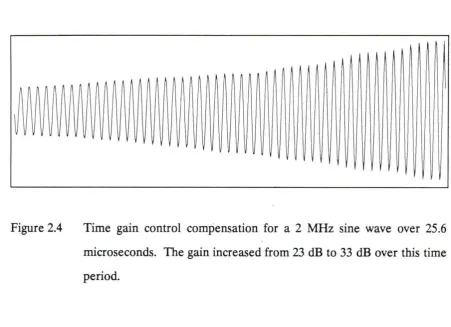
The second amplifier stage has been designed with a variable gain in order to compensate for the attenuation of ultrasound in tissue. The AD600 provides two inputs to control gain of the amplifier stage. A linear increase in voltage between these pins will cause a linear increase in the decibel gain of the amplifier. The variable gain of the second stage uses this feature and it is controlled by a time gain control (TGC) circuit. The TGC circuit is an integrator implemented using an OP-20 (US) manufactured by PMP. The integrator is biased at 2.5 volts and is used to integrate one of the timing signals from the rnicrocontroller. By integrating a step voltage change, the TGC circuit produces a linear ramp. By using this ramp to drive the gain control of the AD600, the amplifier will have an increased gain over time. The time constant of the integrator was chosen to produce a linear ramp with a slope of 0.021 volts per microsecond (V / usec). This yields a time gain control of 2.6 dB per centimeter of tissue that the ultrasound travels through. Figure 2.4 shows

the results of this gain compensation on a 2 MHz sine wave over a 25.6 usec time

period.

Finally, m order to prevent the initial voltage spike (which stimulates the transducer) from saturating the amplifiers, the rnicrocontroller disables the first amplifier stage during the pulsing of the transducer. In addition, diodes D3 and D4 prevent the voltage from exceeding the maximum allowable input voltage for the AD600.

[image:19.572.56.508.67.394.2]

I

Figure 2.4 Time gain control compensation for a 2 MHz sine wave over 25.6 microseconds. The gain increased from 23 dB to 33 dB over this time period.

Analo~ to Di~tal Conversion Analog to digital conversion is accomplished

usmg an eight-bit flash converter, AD9048 (UlO), manufactured by Analog Devices2• _{The clocking of this converter was accomplished using a 20 MHz CMOS}

clock oscillator (U9). The clock output was enabled using one of the timing signals from the microcontroller. This allows the microcontroller to select a window of the reflected ultrasound signal for processing. A low impedance reference voltage is generated using an error amplifier (U15) which drives the base of an emitter follower amplifier (Q2) (Analog Devices, 1989).

The hi~h speed data buffer Since the microcontroller is not capable of

the output of the ADC. A DS2009 (Ul 1), manufactured by Dallas Semiconductor",

was used because it met the required

sons

write time required for a 20 MHz

sampling rate. This component has 512 bytes of memory. Since the output of this

FIFO is at LS-TfL level, and the microcontroller requires HC input levels, a 74HCT540 (U12) was used to convert between the logic levels.

Power supplies All of the circuits are powered by two power supplies

providing + 5 volts and -5.2 volts. A 7805 (U14) voltage regulator is used to produce

a regulated

+

5 volts from a + 9 volt battery source. A 7905.2 (U13) voltage regulator is used to produce -5.2 volts from a -9 volt battery source. In order to conserve energy during idle times, power to some of the circuitry (signal conditioning, ADC, and the data buffer) is turned off by the rnicrocontroller using FET switches Q3, Q4, and QS.

The rnicrocontroller The embedded rnicrocontroller (Motorola5

MC68HC11Al, Ul) controls the precise timing needed to synchronize the transducer pulser and the ultrasound signal sampling, as well as the critical timing of the signal conditioning. In addition, the rnicrocontroller communicates with the high speed data buffer. Finally, the microcontroller has a serial interface which allows the DAB to communicate with an external computer. The microcontroller is wired to operate in bootload mode. This allowed for flexibility during the

4 Dallas Semiconductor, Dallas, TX USA

development of the microcontroller software, and eliminated the need for external memory.

Microcontroller Software Description

The microcontroller software consists of the following five functional blocks: 1) Initializing the microcontroller.

2) Receiving setup commands. 3) Cycling power.

4) Timing the transducer pulsing and data acquisition events. 5) Serially transmitting the ultrasound data.

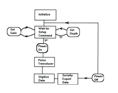
Figure 2.5 shows a flow graph of this code. See Appendix B for a listing of the Motorola 68HC11 source code.

Initializini the rnicrocontroller After the microcontroller is bootloaded, the microcontroller is initialized. First, a region of random access memory (RAM) is allocated as a stack. Next, serial communication with an external computer is set up and enabled. Finally, input/output (I/O) pins are programmed for the appropriate direction (either input or output) and output pins are set to appropriate initial logic levels.

Receivini setup commands Once the microcontroller is initialized, it is put

between the pulsing of the transducer and the start time for digitizing the reflected signal (using the microcontroller line labeled Acquire). This delay number allows the microcontroller (and therefore the user of the microcomputer) to control the depth of the sampling of the ultrasound signal. The actual delay time is equal to the delay number times 0.5 microseconds. This method allows for depth control

between 0 and 127.5 microseconds. Assuming that sound travels approximately

1500 meters/ second (m/ sec) in tissue, the allowable depth control is 0 to 9.6

[image:22.572.91.502.310.634.2]

centimeter (cm), in steps of 0.375 cm.

Figure 2.5

Initialize

Walt for Setup Command

Pulse Transducer

Digitize Data

Set Depth

Serially

Export

Data

During the receiver setup routine, if an ASCII code for a "P" is received, the rnicrocontroller branches to a routine which turns on power, pulses the transducer, and digitizes a portion of the reflected signal.

The third possible setup command is to transmit a gain number. As the name

implies, the gain number allows the microcontroller to vary the gain of the signal

conditioning circuitry. With a 20 MHz sampling rate and a 512 byte FIFO, only 25.6

microseconds of data is stored. Since the TGC circuit generates a voltage ramp with a slope of 0.021 volts per microsecond, the maximum voltage change over 25.6 microseconds is 0.54 volts. However, the AD600 amplifier has a linear decibel gain control over a range of 1.25 volts. Therefore the gain number is used to shift the TGC ramp in time (relative to the data acquisition window) in order to allow the microcontroller (or the microcomputer user) to vary the amplifier gain.

Cyclin~ power An output line of the microcontroller is used to activate the

power switching transistors, which conserves power during idle times. Prior to removing power from unneeded circuits, the microcontroller sets all logic signals which go to these circuits to 0 volts.

Timin~ transducer pulsin~ and data acquisition events The microcontroller

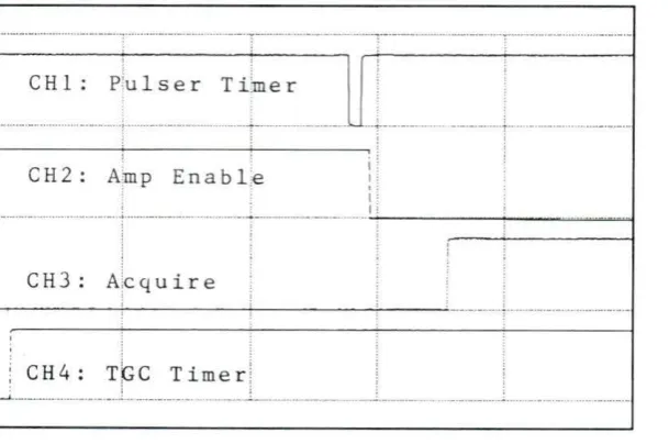
Acquire line (data acquisition windowing), driving the TGC circuit, and disabling the amplifier during pulsing. The fifth microcontroller timing output is used to drive the READ input of the FIFO after data acquisition is complete.

To control the four timing events, the main system counter is read and a setup time is added. Then all four events are setup to occur at an offset from this value. First, the TGC timer is setup to toggle high. Then, a minimum TGC setup time is added. This allows the integrator to get within the valid linear range for the AD600. Then, the gain term is added to allow for shifting the gain within the linear region. Then, this time is used to setup the data acquisition timer (Acquire). Figure 2.6 shows the TGC ramp and the Acquire timer output for a low gain setting and a high gain setting. This ramp shifting allows for programmable gain control using a gain term transmitted from the PC to the DAB.

[image:25.568.88.427.76.539.2]

Figure 2.6

I

. ·1·· t ····-···-····

I I I I

, I

, .. f ·-·-·-·-·

I I I ' I I

CHl : Acquire

Demonstration of TGC ramp shifting (CHl: Acquire signal 2 V /div, CH2: TGC ramp, 0.5 V /div, X-axis is lOusec/div): a) data acquisition starts at a "low gain, b) data acquisition starts at a high gain

[image:26.569.84.430.71.268.2]

Figure 2.7

Figure 2.8

--·---·--·--1--·---·-·-_ . -·--i·-·-··. ________ ... L._ -·-·-· . _________ t. ··-·--·-·-· ·-···---·-·

' CH 1: Amp Ena bile '

; ;

. -·-·-·-·-··· ... --· -·-·-

...

_; _ .. __ ·-·-· -.

---I : i I ;

I '

I

!

---·---·- ··-·-·;--r··-····-·-·---·-· . .. ·-·--:·-···

I ;

I i

I i

... -·-+·

~···

.. ·-·-·-·-·-· ...

I !

I

i i

i ;

. ·-·-·-·-·-···-;-·-·-·--· ---·-·-·-·-·+·

r

I

i

!

!... ····-r-·---.. ... t'" . ... --- -· - · ••

·---1 .

I !

I !

1 CH2i: Pulser; T imer I

. ... r-·-·-·-···:-·-·-·-·-·

'

I i

Pulser timer outputs and amplifier enable output (CHl: amp enable, 2 V / div, CH2: pulser timer, 2V /div, X-axis: 5 usec/ div)

C H 1 : P'u 1 s e r T i:m e r

CH2: Amp Enable

' ;

"''!·-·-·-·-· .... ---·-···1·· •. ·-·-·-·-· ..

-··---I,

,,

..

1;

--- --~ ·· ·-·-·-·-· : ····---· •• ••• · - -·- - · •••• ··---·----. ••• _1 '---~-!

;

C H 3 : A:c q u i r e

I - - - ' - -- - - ' - -- - - - ; -- -

--·-·-·-···-·-·-·-·-···-·-·-·-·-! 1

, CH 4 : Tk;c T ime r !

--'----··••···--·-·-·••·j ·• ••-••·-·-·-·-· I ····-·-·-·-· ·-·· -··-·-·-·-·-· ; ... -·-·-·-···· ·-·-··

[image:26.569.137.442.372.574.2]

PC Description

The PC used in ultrasound data collection was a Toshiba6 _{TlOOOSE notebook}

computer with a standard RS-232 port for serial communication with the DAB. For programing this computer, Microsoft Quick BASIC was used. Appendix C is a listing of this source code.

The PC code has seven functional blocks including: 1) Bootloading the DAB.

2) Setting the gain control variable. 3) Setting the depth control variable. 4) Pulsing a transducer.

5) Receiving the reflected ultrasound data. 6) Displaying this data.

7) Storing the data on a disk for later processing.

Bootloadin~ the DAB The PC code starts by opening a file containing the

assembled microcontroller code and converting this code to byte values. Then, the PC waits for the DAB to be powered up. When the DAB power has been applied, the PC transmits the controller code to the DAB via the serial port.

Settini the ~ain control After bootloading is complete the user is prompted

for a gain setting, which is downloaded to the DAB. After each acquisition the user

may change the gain setting if the need arises.

Settin~ the depth control The current PC code bas 5 pre-programmed depth

settings starting at 1 cm into the tissue with each following acquisition going 1.8 cm deeper then the previous one. This code could easily be modified for different experimental protocols.

Pulsin~ a transducer The ASCil code for a "P" is sent to the DAB to initiate

the pulsing of a transducer.

Receivin~ the reflected ultrasound data Once the pulsing command has been

issued, the PC waits for the DAB to transmit the digitized reflection.

Displayin~ the data In order to provide the user with a pictorial

representation of the received data, the data is display graphically by drawing lines between the data samples.

Storin~ the data Once the data has been displayed, the user is asked if this

data should be stored. If the user responds with a yes, then the user is requested to

provide sample identification. Then the PC stores the raw data, along with the identification, as well as gain information, and depth information on a floppy disk. Once this is complete, the PC waits for the user to request the next sample be taken.

Carcass Data Collection Methods

Ultrasound data was collected at three meat packing plants. All ultrasound

was collected from the dorsal side of the longissimus dorsi between the 12th and 13th ribs using water as a coupling agent between the transducer and the backfat. However, at two of the packing plants, automatic hide pullers were used. This resulted in irregular and inconsistent patterns of trapped air pockets in the backfat. Since the reflection coefficient for air is high, these air pockets lead to irregular and inconsistent data.

Experiments on data collection from the ventral side of the longissimus dorsi were much more consistent; however, the diaphragm blocked the normal grading site of the region between the 12th and 13th ribs. Therefore, all ventral data was taken in the region between the 10th and 11th ribs.

CHAPTER 3 RESULTS AND DISCUSSION

This section presents the results of the designed system; then the limitations of this system are discussed. In addition, an analysis of data acquired in the field is presented. Finally, recommendations for future work are given.

System Results

To evaluate the system, the following characteristics were analyzed:

1) Impulse response.

2) TGC results. 3) Filter results.

4) Power requirements. 5) Cost requirements.

Following the above evaluation, the system's limitations are discussed.

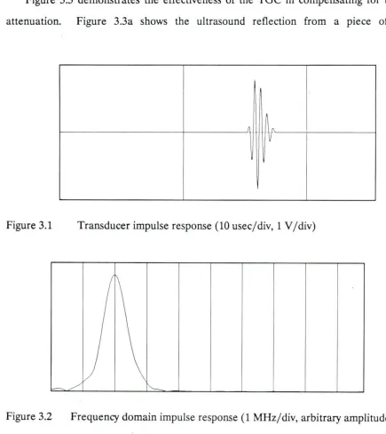
Impulse Response·

From these graphs, the center frequency of the transducer is 2.1 MHz, with a -12dB ·bandwidth of 1.4 MHz.

[image:31.571.49.484.191.679.2]

Time Gain Control Results

Figure 3.3 demonstrates the effectiveness of the TGC in compensating for tissue attenuation. Figure 3.3a shows the ultrasound reflection from a piece of the

[image:31.571.115.477.261.419.2]

t

[image:31.571.94.463.480.638.2]

Figure 3.1 Transducer impulse response (10 usec/ div, 1 V / div)

[image:32.569.118.432.237.438.2]

longissimus dorsi with the TGC connected. Figure 3.3b shows a signal from the same sample with the TGC disconnected. This demonstrates that signals deeper in the tissue can be resolved into more bits than would be possible without the gain compensation. This gain compensation could allow the assessment of the richness of the reflected ultrasound signal.

Figure 3.3

Filter results

[image:32.569.61.480.242.576.2]

Demonstration of TGC effectiveness (X-axis 5 usec/ div, amplitude 1 V / div at DAC): a) Ultrasound reflection from meat sample with TGC; b) Ultrasound reflection from the same meat sample without gain compensation

off of approximately -6 dB per octave. The measured -3 dB high frequency is

approximately 2.5 MHz with a roll off of approximately -12 dB per octave. The analysis

of the impulse response suggests that frequencies beyond 2.7 MHz may contain relevant spectral information; therefore, the low pass cut off frequency should be raised to at

[image:33.571.125.434.282.473.2]

least 3 MHz for this transducer. However, for this experiment, the cutoff frequencies were fixed for all samples. Therefore, comparison of the spectral information of different samples can still be considered legitimate .

Figure 3.4

.

II

•

••

•

II

..

•

•

II

••

••

10000 100000 1000000 10000000

Bode plot generated using a constant magnitude sine wave input (X-axis: frequency in Hz, Y-axis: amplitude in dB with 5 dB/ div scale)

Power requirements

During data acquisition, the DAB draws 118 milliamperes (mA) from the

+

9 V

battery and 132 mA from the -9 V battery. During idle time, the DAB draws 25 rnA

Cost requirements

Appendix F is a list of the materials required for the DAB, as well as an estimate of the cost for each item. These estimates are based on the assumption that components can be purchased in a moderate order size ( 100 at a time). The total estimated cost for

the DAB hardware is $200. Therefore, including the cost of a TlOOSE notebook

computer, a portable ultrasound data acquisition system can be set up for under $1000.

System limitations

Originally, the DAB was designed to accommodate an eight transducer array. This was accomplished by using the microcontroller to select which of the eight outputs of the 74HC138 (U4) would pulse low. These outputs would drive an array of eight

transducers which were multiplexed using an analog 8-1 multiplexer 74HC405 l. The

output of this multiplexer would be fed into the signal conditioning circuitry. However, noise problems occurred in this circuit. The primary cause of this noise was a long path that current had to travel to get from the grounded side of the transducer to the ground plane of the amplifier circuitry. This noise was eliminated by connecting a single transducer directly across the input to the first amplifier stage and its ground plane.

A second problem encountered while developing the DAB was inadequate excitation of the ultrasound transducer. Initially, the regulated

+

5 V supply was used to charge the tuning inductor of the transducer; however, this did not produce enough

ultrasound energy to penetrate much beyond the surface of the tissue. Using the + 9 V

battery instead of the + 5 V produced a much greater sound pulse (voltage spike of 22

penetrating; however, the unregulated voltage was very sensitive to temperature and battery freshness.

Another problem encountered in the field was the difficulty of assuring consistent transducer coupling. Variations in coupling could greatly affect the amount of energy transmitted into and received from the tissue.

Data Analysis

The objective of collecting ultrasound signals is to determine the amount of intramuscular fat (marbling). The magnitude of the reflected signal is reviewed as a possible method for marbling discrimination. A second method looks for shifts in the center frequency and bandwidth in the spectrum of the reflected signals.

Time domain analysis

Figure 3.5 shows the A-mode reflections for two samples. Figure 3.5a shows a highly marbled sample (moderately abundant 60% ), while 3.5b shows a lower marbled sample (slight 50% ). From this figure, it appears that the richness of the reflected signal could be used for grade determination; however, the coupling problem and the unregulated stimulating voltage make statistical analysis impossible. In addition, there appeared to be a large degree of individual variability independent of grade.

Frequency domain analysis

[image:36.573.70.482.96.459.2]

Figure 3.5 A-mode ultrasound reflections viewed from the dorsal side of the longissimus dorsi from 2 cm depth to 5.8 cm: a) sample with marbling score of moderately abundant 60%, b) sample with marbling score of slight 50%

[image:37.570.130.495.194.590.2]

Abundant 100%" (see figure 1.1). Table 3.1 shows the resulting center frequency and bandwidth values and the corresponding marbling scores for 21 carcass samples taken from the ventral side.

Figure 3.6 _{Spectrum of reflected signals (X-axis: 2 MHz/ div, Y-axis relative}

Table 3.1 Marbling score, spectral peak frequency, -12 dB bandlirnits, and -12 dB bandwidth for 21 carcass samples

Marbling Score Low Bandlirnit _{Frequency Frequency} Peak High Bandlirnit _Frequency Bandwidth

23 1211 1875 2930 1719

24 1211 1719 2773 1562

24 1250 2227 2852 1602

25 1487 1719 2812 1325

25 1289 1758 2773 1484

28 1367 1641 2500 1133

28 859 2188 2773 1914

29 1367 2227 3008 1641

29 1289 1875 2734 1445

29 1289 1797 2695 1406

30 1523 1836 2422 899

31 1367 2188 2812 1445

31 1133 2383 2812 1679

31 1328 2188 2617 1289

32 1094 1875 2852 1758

32 1055 2148 2930 1875

32 1406 1875 2773 1367

34 1250 1953 2656 1406

35 1328 1523 2656 1328

36 1328 21 48 2930 1602

[image:38.567.52.508.144.517.2]

40 1172 2109 2734 1562

[image:39.568.132.453.126.553.2]

Figure 3.7

3000 _{• I}

I _{• I}

•

•

I

•

•

•

•

•

2500

•

_•

2000 1500 1000 500 0

20 25 30 35 40

3000 2500 2000

1500

•

•

• I • • I I •

•

•

• •

•

1000 I

•

500 0

20 25 30 35 40

3000

2500

_•

•

_•

_{• • •}

_•

_•

2000

_•

I •

• •

• I

•

1500

•

1000

500

0

[image:40.570.124.430.72.285.2]

20 25 30 35 40

Figure 3.8 Marbling score versus peak frequency (Y-axis is frequency in kHz)

Recommendations

My recommendations would be to implement circuit improvements including: 1) Redesign the transducer array. The noise problem encountered with this

system could be overcome with careful attention to transducer and multiplexer grounding.

2) Provide a regulated stimulus voltage for the transducer pulsing. 3) Improve the cutoff frequencies of the bandpass filter.

4) Develop a method to ensure consistent transducer coupling. 5) Attempt to optimize the circuit for lower power consumption.

Amin, Viren R. 1989. Ultrasonic attenuation estimation for tissue characterization. Masters Thesis. Iowa State University.

Analog Devices. 1989. Data Conversion Products Databook. p3-515.

Anselmo, V. J., J. Clark and P. M. Gammell. 1987. Electronic inspection of beef. JPL

invention R eport NP0-15477 / 4352. (Jet Propulsion Laboratory,

California Institute of Technology, Pasadena, California).

Brethour, John, R. 1990a. Increasing profitability in feedlot cattle with ultrasound

technology. Kansas Agricultural Experimental Station Report of

Progress #597.

Brethour, John, R. 1990b. Relationship of ultrasound speckle to marbling score in cattle. Kansas Agricultural Experimental Station Report of Progress #597.

Chang, Alan. 1991. Utility of the backscattered ultrasound A-mode signal for the quantitative grading of beef. Masters Thesis. Iowa State University.

Feleppa, E. J. and M. Yaremko. 1987. Ultrasonic tissue characterization for diagnosis and monitoring. IEEE Engineering in Medicine and Biology, 18-26.

Gore, J.C. and S. Leeman. 1977. Ultrasonic backscatter from human tissue: a realistic. model. Physics in Medicine and Biology 22:317-326.

Gatenby, J. C., J. C. Hoddinott, and S. Leeman. 1989. Phasing out speckle. Physics in Medicine and Biology 34:1683-1689.

Gupta, V. N, P. K. Bhagat and C. E. Ott. 1982. Ultrasonic characterization of acute

renal failure. Ultrasound in Medicine and Biology 8:249-261.

Haumschild, D. J. and D. L. Carlson. 1983. An ultrasonic Bragg scattering technique

Kuc, Roman, K. Haghkerdar and M. O'Donnell. 1986. Presence of cepstral peak in

random reflected ultrasound signals. Ultrasonic Imaging 8:196-212.

Parks, Bosoon and Dale Whittaker. 1990. Determination of beef marbling score using ultrasound A-scan. American Society of Agricultural Engineers. Paper number 90-6058.

USDA 1965. Official US standards for grades of carcass beef, USDA, C. N. M. S.

Webster, John. 1978. Medical instrumentation application and design. Houghton

Mifflin Company, Boston, 602pp.

Wells P. N. T. 1969. Physical principles of ultrasonic diagnosis. Academic Press, New

York, 12pp.

Whittaker, AD., B. Parks, and B. R. Thane. 1990. Principles of ultrasound and

measurement of intramuscular fat. Department of Agricultural

Engineering Report, Texas A & M University.

Widyaatmadja, Lanny B. 1991. Attenuation measurement of the backscattered

ultrasound A-mode signal for beef grading. Masters Thesis. Iowa State University.

Woods, M. 0 ., and C. A Miles. 1986. Ultrasound speed and attenuation in

ACKNOWLEDGMENTS

\100

\ISS \IRH \IRL HODA HODO RST XIRQ IRQ PD2 PD3 PD4 PD5 RXO

~

~

TXD

NOT ES :

E

NOTE 1 ~ -9V

1 > 5MITCH1 CS1A ANO 518 > 15 A DOUBLE POLE OOU8LC THROW SMJTCH r o R THC DAB HAI H ,.OMER.

• microcontroller.

*This code is used for digitizing an ultrasound signal and exporting this data serially.

•set assembler variables

DELAY EQU $0000

TRAN EQU $0002

GAIN EQU $0003

PORTA EQU $()()

PORTO EQU $08

PORTE EQU $0A

DORO EQU $09

CFO RC EQU $OB

OClM EQU $0C

OClD EQU $00

TCNT EQU $OE

TOCl EQU $16

TOC2 EQU $18

TOC3 EQU $1A

TOC5 EQU $1E

TCTLl EQU $20

TFLGl EQU $23

PACTL EQU $26

BAUD EQU $2B

SCCR2 EQU $20

SCSR EQU $2E

SCIINT EQU $C4

XMIT EQU $2F

RCV EQU $2F

RCVSET EQU $4000

WIDTH EQU $20

*START OF THE MAIN PROG *SETUP STACK AND INDEX

LDS #$00FF

LDX #$1000

CLRA

WAA

#lC STAA TRAN

LDAA #$30 SET BAUD TO 9600

STAA BAUD,X

WAA

#$0C ENABLE RS-232 COM

STAA SCCR2,X

LDAA #$3C SET UP PORT D FOR OUTPUT

STAA DDRD,X

WAA

#$80

STAA OClD,X SEND TIMER 1 HIGH

STAA PACIL,X SET UP TIMER 1 AS OUTPUT

STAA OClM,X SET PORTA PIN 7 AS TIMER 1 OUTPUT

WAA

#$20

STAA PORTD,X TURN POWER OFF

BRA WAIT

ON

LDAB #$B2 STAB TCTLl,X LDAB #$E8 LDAA #$1C

STAB CFORC,X FORCE: OC2=LOW OC3=HIGH

STAA PORTD,X

WAA

#$30

STAA PORTA,X

LDY #$FOOO DELAY TO ALLOW POWER TO STABLIZE

DUHLAY DEY

BNEDUHLAY RTS

DEPTI-1

*Get delay depth from computer via RS-232

BSR SERIAL

LDAB RCV,X DOWNLOAD DELAY

STD DE1AY

BRA WAIT

*SUBROUTINE: SOFTWARE POLLING FOR RS-232 RCV DATA SERIAL

LDAA SCSR,X TAB

ANDA #$20

BEQ SERIAL

RTS

*WAIT FOR A PULSE OR A DEPTI-I COMMAND FROM THE COMPUTER WAIT

BSR SERIAL

LDAA RCV,X REGURGITATE

LDAB SCSR,X ANDB #$CO

BEQ REGURGITATE

STAA XMIT,X CMPA #$50

BEQ GO

CMPA #$44

BEQ DEPTH

STAA GAIN

BRA WAIT

GO

BSR ON TURN POWER ON

PULSE

LDD TCNT,X

ADDD #$50

STD TOC5,X

ADDD #$380 ADDB CURVE) ADCA STD GAIN #$00 TOC2,X

GET CURRENT COUNT

ADD A LITTLE TIME TO SET UP TIMERS START INTEGRATION OF TIMER 5 (TGC) ADD MINIMUM WAIT FOR VALID TGC LEVEL WAIT FOR GAIN COUNT (IE, SHIFT UP GAIN

SUBD DELAY PULSE TRAN 'DELAY BEFORE DATA ACQ PSHA

PSHB

SUBD #WIDTH

STD TOC3,X TURN ON CURRENT INTO THE TRANSDUCER

LDAA #$D3

STAA TCfLl,X SET TIMER TO APPROPRIATE MODE

PULB

LDAA #$20

STAA TFLGl,X CLEAR ANY PENDING TIMEOUTS

CHECK

LDAA TFLGl,X CHECK FOR TIMER 3 TIMEOUT

•

(IE. TRANSDUCER IS BEING PULSED)

ANDA #$20

BEQ CHECK

PULA

STD TOC3,X PULSE THE TRANSDUCER

ADDD #$15

STD TOCl,X ENABLE INPUT TO THE AMP AFTER PULSE

CLRA

STAA OClD,X

LDAA #$F3 KEEP TIMERS 2,3,5 HIGH UNTIL DATA IS

DOWNLOADED STAA TCfLl,X

LDAB DELAY WHEN DELAY IS OVER, DATA IS BEING TAKEN

ASRB ASRB ASRB CLRA XGDY ABOVE

DEY DELAY TIME TO ALLOW DATA ACQUSITION TO

START

*READ FIFO

LDY #$0200

LDAB #$30

CLRA

STAA PORT~X

STAB PORT~X

STAA PORT~X

STAB PORT~X

READING

LDAA SCSR,X ANDA #$CO

BEQ READING

CLRA

STAA PORT~X

LDAA PORTE,X

STAB PORT~X

STAA XMIT,X DEY

BNE READING

LDAA #$80 STAA OClD,X LDAA #$B2 STAA TCfLl,X LDAA #$E8 STAA CFORC,X • LDAA TRAN • ADDA #$04 • STAA TRAN • STAA PORTD,X • CMPA #$20

• BNE PULSE

PULSED • CLRA

• STAA TRAN

BSR OFF

JMP WAIT

READ FIFO 512 TIMES

SET READ\ LINE LOW READDATA

SET READ\ LINE HIGH SEND DATA TO COMPUTER

RE-INITIALIZE TIMER 1

RE-INITIALIZE TIMER 2 AND 3

SET UP MUX & DEMUX FOR NEXT TRANSDUCER

OFF

CLRB

LDAA #$20

'Microcomputer source code

DECLARE FUNCTION ASCIITOINT% (CHARACfER AS STRING) 'used to aquire data 5-19-92 thru 6- on cattle. This

version has 5 consecutive depths, the user selects the gain for the first depth

CONSTyes = 1 CONST no= 0 CONST delay = 1000 DIM value(512, 10) DIM software%(255)

'open the file that contains the assembled HCl 1 code. OPEN "a:\HCll \ bootload" FOR INPUT AS #2 count% = 0

'convert the ASCII hex nibbles to integer numbers

DO WHILE NOT EOF(2) AND count% < 256

first$ = INPUT$(1, #2) second$ = INPUT$( 1, #2)

'convert the first and second (ASCII) hex digits to an' integer( =number)

number% = 16 • ASCIITOINT(first$)

+

ASCIITOINT(second$) software%( count%) = number%

count% = count% + 1

LOOP

'pad the bootload code to 256 bytes (207= 'STOP' for HCll) FOR i% = count% TO 255

software%(i%) = 207

NEXT

CLOSE#2

'open serial port and wait for a break character from HCl 1 ON ERROR GOTO handler

OPEN "COM1:1200,N,8,l,cd0,cs0,ds0,RB512,BIN" FOR RANDOM AS 1

PRINT "Waiting for power to be applied to board (HCl 1 break character)"

breaking%

=

yes

break$

=

INPUT$(1, #1)

breaking%

=

no

'send HCl 1 the character $FF to set BAUD to 1200 PRINT #1, CHR$(255);

CLS

PRINT "Break received"

junk$

=

INPUT$(LOC(l), #1)

'bootload the HCll

FOR i%

=

0 TO 255

PRINT #1, CHR$(software%(i%)); NEXT

CLOSE#l

OPEN "COM1:9600,N,8,1,cd0,cs0,ds0,RB512,BIN" FOR RANDOM AS 1 CLS

path$

=

"A:\DATA" CHDIR path$

PRINT : PRINT

'determine what the highest extention A:\DATA\RAWDATA.xxx is extention%

=

-1

alldone%

=

no

repeater:

extention%

=

extention%

+

1

a$

=

CHR$(((extention% \ 100) MOD 10) + 48)

b$

=

CHR$(((extention% \ 10) MOD 10)

+

48)

c$

=

CHR$((extention% MOD 10) + 48)

exten$

=

a$ + b$ + c$

FILES path$ + "\RA WDAT A." + exten$

IF alldone%

=

no THEN GOTO repeater

file$ = path$ + "\RA WDA TA." + exten$

PRINT : PRINT "Data will be stored in: "; file$: PRINT

PRINT : PRINT "Each subsequent data file will add one to the extension": PRINT

FILES"•.•" PRINT : PRINT

'determine the number of locations that the user wants

PRINT "Please enter the number of transducer locations for each animal"; INPUT": ", locations%

IF ((locations% < 1) OR (locations% > 10)) THEN locations = 6

'trigholdoff:

'INPUT "please enter delay (in centimeters) ... ", dist! 'PRINT : PRINT

dist! = 1

IF dist! < .5 THEN dist! = .5 dlay% = dist! • 26.6667

IF dlay% > 255 THEN dlay% = 255 usec! = dlay% • .5

dist! = usec! • .075

gainset:

INPUT "Please enter gain as a percentage (0 - 100) ... ", gain% IF gain% < 0 THEN gain% = 0

IF gain% > 100 THEN gain% = 100 gain% = gain% + gain%\ 2

IF ((gain% = 68) OR (gain% = 80)) THEN gain% = gain% + 1 PRINT #1, CHR$(gain%);

junk$ = INPUT$(1, #1)

CLS

again: SCREEN 0

file$ = path$ + "\" + "RA WDATA." + exten$

PRINT ''Type 'G' to change the gain" PRINT ''Type 'Q' to quit"

INPUT "Position transducer at location 1 and hit ENTER to acquire data ... ", j$

CLS

j$ = LEFTIU$, 1)

IF (U$ = "g") OR US = "G")) THEN GOTO gainset IF (U$ = "q") OR US= "Q")) THEN END

OPEN file$ FOR OUTPUT AS #3 LEN = 4608 PRINT #3, "Number of locations = ";locations%

FOR position% = 1 TO locations%

nextdelay% = dlay% nextgain% = gain%

'for 5 different depths acquire signals from the transducer FOR num% = 1 TO 5

PRINT #1, CHR$(&H44);

FOR k = 0 TO 100: NEXT

IF (nextdelay% > 255) THEN nextdelay%

=

255

PRINT #1, CHR$(nextdelay%); junk$ = INPUT$(1, #1)

IF (nextgain% > 200) THEN nextgain%

=

200

IF ((nextgain%

=

68) OR (nextgain%

=

80)) THEN nextgain%

=

nextgain%

+

1

PRINT #1, CHR$(nextgain%); junk$ = INPUT$(1, #1)

PRINT #1, CHR$(&H50); junk$ = INPUT$(1, 1)

DO

count%

=

LOC(l)

'tell HCl 1 to pulse transducers

LOOP UNTIL count%

=

512

nextdelay% = nextdelay%

+ (

1.8 * 26.6667) \ 1 nextgain % = nextgain % + 50

NEXT

SCREEN2

FOR index% = 0 TO 4

PRINT #3, info$(index% + 1) 'store data for each depth

FOR i% =OTO 511

value(i%, index%) = ASC(MID$(info$(index%

+

1), i%

+

1, 1))

'IF i% > 0 THEN LINE (i%, 50 + value(i% - 1, index%)/ 2)-((i% + 1), 50

+

value(i%, index%)/ 2)

NEXT NEXT

FOR index% = 0 TO 4

FOR i% = 0 TO 505 STEP 5 max= 0

index%)

index%)

min= 255

FORk% = OT04

IF (value(i% + k%, index%) > max) THEN max = value(i% + k%,

IF (value(i% + k%, index%) < min) THEN min = value(i% + k%,

NEXT

x% = (i% \ 5) + (index% * 100)

yl % = (35 * (index% + 2) - maxold / 5) y2% = (35 * (index% + 2) - max / 5)

IF i% > 0 THEN LINE (x%, yl %)-(x% + 1, y2%)

maxold =max

zl % = (35 * (index%

+

2) - minold / 5) z2% = (35 * (index%

+

2) - min / 5)

IF i% > 0 THEN LINE (x%, z1%)-(x% + 1, z2%)

minold =min NEXTi%

position%

+

1; "and";

INPUT "hit ENTER ",junk$ CLS

NEXT position%

INPUT "Do you wish to save this data (Y or N)? ", save$

save$

=

LEF1'$(save$, 1)

IF ((save$

=

"n") OR (save$

=

"N")) THEN CWSE#3

GOTO again END IF

PRINT #3, "gain count

=

";gain%; " out of 200" PRINT #3, "first delay

= ";

dlay%

PRINT #3, "data spacing

=

I.Bern"

extention%

=

extention%

+

1

a$

=

CHR$(((extention% \ 100) MOD 10) + 48)

b$

=

CHR$(((extention% \ 10) MOD 10) + 48)

c$

=

CHR$(( extention% MOD 10) + 48)

exten$

=

a$ + b$ + c$

'CLS

PRINT : PRINT "Data has been stored in "; file$: PRINT

PRINT : PRINT "Please type identification information followed by ENTER."

PRINT : PRINT "Note: this information will appear in the file exactly as you type it." INPUT "IDENTIFICATION > ", I DENT$

PRINT #3, IDENT$

CLOSE #3

GOTO again

SELECT CASE ERR CASE53

'file not found

alldone% = yes 'no more RA WDAT A.xxx, so I'm done

RESUME NEXT CASE 57

IF breaking%

=

yes THEN

RESUME NEXT ELSE

PRINT."Device I/ O error"

FOR kk%

=

0 TO 10: PRINT CHR$(7); : NEXT

RESUME END IF CASE ELSE

CLS

'RESUME

PRINT "I've fallen and I can't get up"

FOR kk%

=

0 TO 10: PRINT CHR$(7): NEXT

PRINT "try me again soon ... "

PRINT : PRINT "type GO to run again"

END

FUNCTION ASCIITOINT% (CHARACTER AS STRING)

temp%= ASC(CHARACfER$)

IF ((temp% > 47) AND (temp% < 58)) THEN temp% = temp% - 48

IF ((temp% > 64) AND (temp% < 71)) THEN temp% = temp% - 55

ASCIITOINT% = temp%

'this program takes an input file, finds the 512 FIT, smooths this spectrum then calculates and stores the peak frequency, and -12 dB bandlimits DECIARE SUB moveave (spectrum!(), smooth!(), n%)

DECIARE SUB BITRV (n%, XR!(), XI!())

DECIARE SUB R2FIT (n%, XR!(), XI!(), WR!(), WI!()) DECIARE SUB Wf ABLE (n%, WR!(), WI!())

DIM XR!(512), XI!(512), WR!(512), WI!(512), mag!(512), angle!(512), spec!(512) DIM num%(512)

n% = 512

pi = 3.14159265#

k

=

11

SCREEN 9

CLS

COLORk

OPEN "d:\ freq_tbl" FOR OUTPUT AS #2

top:

INPUT "Please enter the file you wish to process ", file$ OPEN file$ FOR INPUT AS #1

'for all five depths FORj% = 1TO5

ave# = 0

FOR i% = 1 TO n%

INPUT #1, num%(i%)

ave# = ave# + num%(i%) / n%

NEXTi%

IFj% = 2THEN

' for the second depth remove TGC effects and DC bias count% = 0

FOR i% = 1 TO n%

count% = count% + l

XR!(i%) = (num%(i%) - ave#) / ((1.00224754#) " count%)

IF (i% > 1) THEN LINE (i%, 100 - (126 - num%(i% - 1)) / 2)-(i% + 1,

END IF

IF j%

=

2 11-IEN

'for the second depth: find the FIT CALL WfABLE(n%, WR!(), WI!())

CALL R2FFf(n%, XR!(), XI!(), WR!(), W1!()) CALL BITRV(n%, XR!(), XI!())

'convert REAL-IMAGINARY to polar

FOR i% = 1 TO 512

mag!(i%) = SQR(XR!(i%) * XR! (i%) + XI! (i%) * XI!(i%))

IF (XR!(i%) > 0) THEN angle!(i%) = ATN(XI!(i%) / XR!(i%))

IF ((XR!(io/o) < 0) AND (XI!(i%) < 0)) THEN angle!(i%) = ATN(XI!(i%) / XR!(i%)) - pi

IF ((XR!(i%) < 0) AND (XJ!(i%) > = 0)) THEN angle!(i%) = ATN(XI!(i%) /

XR! (i%)) + pi

IF ((XR!(i%) = 0) AND (XI!(i%) > 0)) THEN angle!(i%) = pi / 2

IF ((XR!(i%) = 0) AND (XI!(i%) < 0)) THEN angle! (i%) = -pi / 2 NEXTi%

CALL moveave(mag! (), spec!(), 5) 'find peak frequency

max = 0

peak% = 0

FOR i% = 1 TO n% / 2

IF spec!(i%) > max THEN

max = spec!(i%) peak% = i% END IF

NEXT

'find -12 dB low cutoff low%= 0

i%

=

0

DO

IF spec!(i%) > max • .25 THEN low% = i%

i% = i% + 1

'find -12 dB high cutoff

high% = 0

i% = n% /2 DO

IF spec!(i%) > max• .25 THEN high% = i%

i% = i%- 1

LOOP UNTIL ((i% = 0) OR (high% < > 0))

low% = low% • 39.0625 peak% = peak% • 39.0625 high% = high% • 39.0625 PRINT low%, peak%, high%

'display spectrum FORi% = 2T0256

LINE (i% • 2, 320 - spec!(i% - 1) / 25)-(i% • 2 + 2, 320 - spec!(i%) / 25)

LINE (i% • 2, 220 - mag!(i% - 1) / 25)-(i% • 2 + 2, 220 - mag!(i%) / 25)

NEXT END IF NEXTj%

FOR i% = 1TO5

LINE INPUT #1, st$ PRINT st$

NEXT

INPUT "enter grade number > ", gr% PRINT #2, gr%, low%, peak%, high%

SUB BITRV (n%, XR!(), XI!())

'@@@@@@@@@@@@ SUBROUTINE BIT REVERSAL FOR FIT

@@@@@@@@@@@@

'SUB BITRV (N%, XR!(), XI!()) j%

=

1

N1%

=

n% - 1

FOR i%

=

1 TO N1%

IF (i% >

=

j%) GOTO KEND2

temp!

=

XR!U%)

XR!U%)

=

XR!(i%)

XR!(i%)

=

temp!

temp!

=

XI!U%)

XI!U%) = XI!(i%)

XI!(i%)

=

temp!

KEND2:

k%

=

n%

I

2 KGEJ:

IF (k% >

=

j%) GOTO JPLK

j%

=

j% -k%

k%

=

k%

I

2 GOTO KGEJ JPLK:

j%

=

j% + k% NEXTi%

END SUB

SUB moveave (spectrum!(), smooth!(), n%)

place%

=

n% \ 2 + 1

FOR i%

=

0 TO place%

spectrum!(i%)

=

0

smooth!(i%)

=

0

NEXT

FOR i%

=

place% TO 512 - place%

FOR j% = i% - n% \ 2 TO i% + n% \ 2

smooth!(i%) = smooth!(i%) + spectrum!U%) / n% NEXT

NEXT

END SUB

SUB R2FFf (n%, XR!(), XI!(), WR!(), WI!())

'@@@@@@@@@@@@ RADIX-2 DECIMATION-IN-TIME FIT

@@@@@@@@@@@@@ [ ]

'SUB R2FFf (N%, XR!(), XI!(), WR!(), WI!())

FOR P% = 1 TO 15 M% =P%

N2% = 2 AP%

IF (n% = N2%) GOTO start NEXTP%

PRINT, "N, IS NOT A POWER OF 2" STOP

start:

N2% = n%

FOR i% = 1 TOM% N1% = N2% N2%

=

N2%/2 11% = 1

12% = n% / N1% FORj% = 1 TO N2%

C!

=

WR!(l1%) S!

=

WI!(I1%) 11% = 11%

+

12%

FOR k% = j% TO n% STEP Nl % L% = k% + N2%

Xl!(k%)

=

XI!(k%) + XI!(L%)

XR!(L%)

=

C! • TEMPR!

+

S! •TEMPI!

Xl!(L%)

=

C! •TEMPI! - S! • TEMPR!

NEXTk% NEXTj% NEXTi% END SUB

SUB Wf ABLE (n%, WR!(), WI!())

'@@@@@@ GENERA TING SINE AND COSINE VALUES FOR FIT @@@@@@'

'SUB WfABLE (N%, WR!(), WI!())

WN!

=

6.2831853# / (n% • 1!)

FOR k%

=

1 TO n%

PHI!

=

WN! • (k% - 1)

WR!(k%)

=

COS(PHI!)

WI!(k%)

=

SIN(PHI!)

Bill Of Materials June 15, 1992 8:44:37 Page 1

Item Quant Reference Price Discription

1 1 BTl 0.95 9V Battery

2 1 BT2 0.95 -9V Battery

3 4 Cl,ClO,Cl l,Cl2 0.40 0.1 uF Cap

4 1 C2,Cl5 0.10 4.7uF Cap

5 1 C3 0.10 lUuF Cap

6 3 C4,C5,C6 0.30 22pF Cap

7 3 Cl3,Cl4,Cl6 0.30 O.luF Cap

8 1 C7 0.10 O.luF Cap

9 1 C8 0.10 .OluF Cap

10 1 C9 0.10 .OOluF Cap

11 1 C15 0.10 4.7uF Cap

12 1 Cl7 0.10 .047uF Cap

13 3 Dl,D2,D3 0.05 IN4148 Diode

14 1 D4 0.15 4.3V ZENER

15 I Ql 0.20 MOSFET N chan

16 1 Q2 0.15 2N3906 Transistor

17 3 Q3,Q4,Q5 1.20 MOSFET P chan

18 2 Rl,R5 0.04 I kohm Resistor

19 2 R2,R3 0.04 1.2 kohm Resistor

20 1 R4 0.02 10 Mohm Resistor

21 1 RIO 0.02 1.2 kohm Resistor

22 1 Rll 0.02 8.2 kohm Resisitor

23 2 RI2,R14 0.04 4 7 ohm Resistor

24 I RI3 0.02 10 ohm Resistor

25 2 RI5,R16 0.04 100 kohm Resistor

26 I R6 0.02 820 ohm Resistor

27 1 R7 0.02 22 kohm Resistor

28 I RS 0.02 27 kohm Reistor

29 1 R9 0.02 560 kohm Resistor

30 I R17 0.02 100 ohm Resitor

31 I TRI 30.00 TRANSDUCER

32 1 Ul 20.00 MC68HCI I microcontroller

34

35 1 U4 0.40 74HC138 Decoder

36 2 U5,U15 2.00 OP200pArnp

37 1 U6 20.00 AD600 Amplifier

37.5 1 U7 0.69 TLE2426 Rail divider

38 1 U8 2.50 AD847 Amplifier

39 1 U9 2.50 20MCLOCK

40 1 UlO 25.00 AD9048ADC

41 1 Ull 5.00 Dallas FIFO

42 1 U12 1.00 74HCT540

43 1 U13 0.60 7905.2 Regulator

44 1 U14 0.60 7805 Regulator

45 1 Yl 1.12 8.0M Xtal