https://doi.org/10.5194/angeo-36-841-2018 © Author(s) 2018. This work is distributed under the Creative Commons Attribution 4.0 License.
Statistical analysis of the correlation between the equatorial
electrojet and the occurrence of the equatorial ionisation
anomaly over the East African sector
Patrick Mungufeni1, John Bosco Habarulema2,3, Yenca Migoya-Orué4, and Edward Jurua1
1Mbarara University of Science and Technology, P.O. Box 1410 Mbarara, Uganda
2South African National Space Agency (SANSA) Space Science, Hermanus 7200, South Africa 3Department of Physics and Electronics, Rhodes University, Grahamstown 6140, South Africa
4T/ICT4D laboratory of the Abdus Salam International Center for Theoretical Physics, 34151 Trieste, Italy
Correspondence:Patrick Mungufeni ([email protected])
Received: 11 November 2017 – Revised: 8 May 2018 – Accepted: 23 May 2018 – Published: 13 June 2018
Abstract.This study presents statistical quantification of the correlation between the equatorial electrojet (EEJ) and the occurrence of the equatorial ionisation anomaly (EIA) over the East African sector. The data used were for quiet geo-magnetic conditions (Kp ≤3) during the period 2011–2013. The horizontal components, H, of geomagnetic fields mea-sured by magnetometers located at Addis Ababa, Ethiopia (dip lat. ∼1◦N), and Adigrat, Ethiopia (dip lat. ∼6◦N), were used to determine the EEJ using differential techniques. The total electron content (TEC) derived from Global Nav-igation Satellite System (GNSS) signals using 19 receivers located along the 30–40◦longitude sector was used to deter-mine the EIA strengths over the region. This was done by determining the ratio of TEC over the crest to that over the trough, denoted as the CT : TEC ratio. This technique neces-sitated characterisation of the morphology of the EIA over the region. We found that the trough lies slightly south of the magnetic equator (0–4◦S). This slight southward shift of the EIA trough might be due to the fact that over the East African region, the general centre of the EEJ is also shifted slightly south of the magnetic equator. For the first time over the East African sector, we determined a threshold daytime EEJ strength of∼40 nT that is mostly associated with promi-nent EIA occurrence during a high solar activity period. The study also revealed that there is a positive correlation be-tween daytime EEJ and EIA strengths, with a strong positive correlation occurring during the period 13:00–15:00 LT. Keywords. Ionosphere (equatorial ionosphere)
1 Introduction
One of the factors that determines the distribution of ambient ion and electron density in the low-latitude F region iono-sphere is the verticalE×B drift, which is roughly directly proportional to the equatorial electrojet (EEJ) during daytime (Anderson et al., 2002). The daytime EEJ is a narrow band of enhanced eastward current flowing in the 100–120 km al-titude region within±3◦latitude of the dip equator (Chap-man, 1951; Rastogi, 1974). The horizontal configuration of the Earth’s magnetic field at the dip equator leads to the in-hibition of the Hall current. The resulting increase in Cowl-ing conductivity produces the EEJ (Abdu, 1992; Hajra et al., 2009). The EEJ current reverses and flows in a westward di-rection in most cases during quiet geomagnetic and low solar activity conditions as well as during solstice months (Gouin and Mayaud, 1967; Reddy, 1989). This phenomenon is re-ferred to as the counter electrojet (CEJ).
The large enhancements in electron densities on either side of the magnetic equator significantly affect radio fre-quency signals passing through the ionosphere and ground-to-ground high-frequency communication systems (Ander-son et al., 2004). Due to such problems, several studies have been undertaken to understand the influence of the EEJ on the development of the EIA. Most of the studies related to the development of the EIA and EEJ have been done over American and Indian longitude sectors (Sethia et al., 1980; Chakraborty and Hajra, 2009; Hajra et al., 2009; Zhang et al., 2009; Yizengaw et al., 2010; Venkatesh et al., 2015; Rodriguez-Zuluaga et al., 2016). There are also some stud-ies that have used global data to study the morphology of the EIA. For instance, Yue et al. (2015) derived peak elec-tron density in the F2 layer (NmF2) from the Global Po-sition System (GPS) Radio Occultation (RO) observations made by the Constellation Observation System for Meteo-rology, Ionosphere and Climate (COSMIC) mission to study the morphology of the EIA statistically during 2006–2014. They found thatNmF2 increases more significantly with so-lar activity in the crest region than that of the trough region. The ratio of NmF2 at the crest to that at the trough has one peak in the noontime and another around the time of occur-rence of the pre-reversal enhancement (PRE) of the zonal electric field. The ratios are smaller during May–August than other months for all the local times (LT). Rush and Rich-mond (1973) also used global data to investigate the rela-tionship between the EIA and the strength of the EEJ. They found that the correlation coefficients between hourly param-eters that define development of the EIA and the midday EEJ strength tend to maximise between 13:00 and 16:00 LT. On a seasonal basis, the correlation coefficients tend to minimise around the June solstice.
However, there are a few studies that have used data over the African region to examine occurrence of the EIA during geomagnetically disturbed (e.g. Yizengaw et al., 2010; Ol-wendo et al., 2015) and quiet conditions (Bolaji et al., 2017). The study by Bolaji et al. (2017) used data during quiet ge-omagnetic and low solar activity conditions in the year 2009 to confirm the roles of the EEJ and integrated EEJ (IEEJ) in determining the hemispheric extent of the EIA crest over African mid-latitudes and low latitudes. They reported that, in the Southern Hemisphere, EIA crests can be seen in the magnetic latitudes ranging from about 17 to 19◦S.
At the moment, there is no statistical quantification of the correlation between the EEJ strength and the forma-tion/development of the EIA over the African sector. There-fore, this study focused on statistically quantifying the cor-relation between daytime EEJ strength and the occurrence of the EIA over the East African sector during the high solar activity years of 2011–2013. The method we used necessi-tated searching for locations of the trough and crest of the EIA over the region. The data that were used in this study are described in Sect. 2.
20 25 30 35 40 45 50
-40 -30 -20 -10 0 10 20
Longitude o
L
a
ti
tu
d
e
o
ETHI
AAE
RBAY MOIU ADIS
NEGE
RCMN ARMI
TANZ MAL2 MBAR
ARSH SHEB
NAZR BDMT
EBBE
TUKC DEBK
DODM
SHIS
MZUZ
ZOMB
[image:2.612.347.509.68.374.2]TDOU
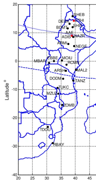
Figure 1.A map showing data sites. The red and black dots
indi-cate the locations of the magnetometers and the UNAVCO stations, respectively. The dotted and dashed lines represent the magnetic equator and the southern crest of the EIA, respectively.
2 Data and analyses 2.1 EEJ data
Table 1.Sites of GNSS receivers and magnetometers used in the study.
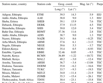
Station name, country Station code Geog. coord. Mag. lat (◦) Purpose
Long (◦) Lat (◦)
Adigrat, Ethiopia ETHI 39.5 14.3 5.9 EEJ
Addis Ababa, Ethiopia AAE 38.8 9.0 1.3 EEJ
Sheba, Eritrea SHEB 39.1 15.9 7.6 TEC
Debarek, Ethiopia DEBK 37.9 13.15 4.5 TEC
Shimsheha, Ethiopia SHIS 39.0 12.0 3.4 TEC
Bahir Dar, Ethiopia BDMT 37.36 11.6 2.8 TEC
Addis Ababa, Ethiopia ADIS 38.7 9.0 1.3 TEC
Nazret, Ethiopia NAZR 39.3 8.6 −0.25 TEC
Arba Minch, Ethiopia ARMI 37.6 6.1 −3.13 TEC
Negele, Ethiopia NEGE 39.6 5.3 −3.7 TEC
Eldoret,Kenya MOIU 35.4 0.5 −8.93 TEC
Entebbe, Uganda EBBE 32.46 0.05 −9.5 TEC
Nairobi, Kenya RCMN 36.89 −1.22 −10.72 TEC
Malindi, Kenya MAL2 40.2 −3.0 −12.4 TEC
Arusha, Tanzania ARSH 36.7 −3.4 −13.04 TEC
Dodoma, Tanzania DODM 35.8 −6.2 −16.6 TEC
Tukuyu, Tanzania TUKC 33.7 −9.3 −19.5 TEC
Mzuzu, Malawi MZUZ 34.0 −11.4 −21.9 TEC
Zomba, Malawi ZOMB 35.3 −15.4 −26.1 TEC
Thohoyandou, South Africa TDOU 30.4 −23.1 −33.8 TEC
Richards Bay, South Africa RBAY 32.0 −28.8 −38.65 TEC
determine either EEJ or total electron content (TEC). Later in Sect. 2.2, we explained the appropriateness of high solar activity data during 2011–2013 that were used in this study.
In order to cater for the different offset values of differ-ent magnetometers, the baseline value HB of each day was
subtracted from the values ofH(Yizengaw et al., 2014). For each day, values ofH measured at a particular station during 23:00–23:59 LT were averaged to give theHBvalue for that
day. The values obtained for a specific station after subtract-ingHBfromHwere denoted asHS. To obtain the EEJ (1H),
theHSvalues calculated at ETHI were subtracted from those
of the corresponding days that were calculated at AAE. Most studies on the EEJ report the peak of the diurnal EEJ around 12:00 LT (Gouin, 1962; Venkatesh et al., 2015; Yizengaw et al., 2014; Subhadra Devi and Unnikrishnan, 2014). In line with this information, the daytime EEJ strength for each day in this study was represented by the mean of the EEJ dur-ing the period 10:00–13:00 LT, when the peak of the daytime EEJ is expected to occur.
2.2 Determination of EIA strength
The EIA strengths were calculated using data obtained from Global Navigation Satellite System (GNSS) receivers along the 30–40◦longitude sector of Africa. The stations are repre-sented with black dots in Fig. 1. The latitude range of the stations considered were mainly restricted to the south of the dip equator. However, a few stations slightly north of the dip equator were considered to allow us to locate the
trough of the EIA over the region. The Receiver INdepen-dent EXchange (RINEX) data files of the receivers were obtained from the University NAVstar COnsortium (UN-AVCO) website (ftp://data-out.unavco.org/pub/rinex/, last access: 15 September 2017). Data of geomagnetically quiet days (Kp≤3) were considered. The development of the EIA during disturbed conditions could be examined in a separate study since it involves additional mechanisms such as the prompt penetration of magnetospheric electric fields and the disturbance dynamo electric fields.
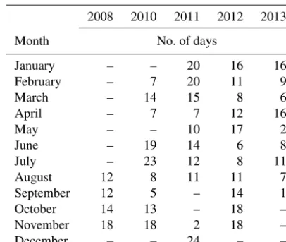
Table 2 shows the number of geomagnetically quiet days when the magnetometers at ETHI and AAE and seven of the GNSS receivers (ADIS, ARMI, MOIU, RCMN, EBBE, MAL2 and DODM) listed in Table 1 were simultaneously operational. Dashes in the table depict unavailability of data. Considering the fact that the formation of the EIA depends on solar activity (e.g. Yue et al., 2015), we grouped the data into low (2008 and 2010) and high (2011–2013) solar activ-ity periods. This grouping might minimise the effect of solar activity on the correlation between EIA and EEJ. For statis-tical analysis, it appears that the amount of data of low solar activity period shown in Table 2 is not sufficient. Therefore, in this study, we used data of the high solar activity years of 2011–2013.
Table 2.Number of days in which magnetometers and some GNSS receivers used were simultaneously operational.
2008 2010 2011 2012 2013
Month No. of days
January – – 20 16 16
February – 7 20 11 9
March – 14 15 8 6
April – 7 7 12 16
May – – 10 17 2
June – 19 14 6 8
July – 23 12 8 11
August 12 8 11 11 7
September 12 5 – 14 1
October 14 13 – 18 –
November 18 18 2 18 –
December – – 24 – –
we used data of satellites with elevation angles greater than 25◦ (Mungufeni et al., 2016). The daily VTEC data were analysed in two ways. In the first analysis, we computed monthly mean TEC over a station as described in the follow-ing procedure. The daily VTEC data for all the days within the study period were binned according to months. There-fore, 12 monthly bins were formed from the data during the period 2011–2013. The monthly bins were further binned ac-cording to LT. The mean values of the LT bins were deter-mined to yield monthly mean TEC with 30 s resolution. In the second analysis, we computed the EIA strengths. Vari-ous studies have represented EIA strength in many ways, in-cluding (i) computing the difference of TEC measured at the crest and that at the trough (Sastri, 1982), (ii) determining the normalised difference of TEC measured at the crest and that measured at the trough (Sastri, 1982), (iii) simply using the peak of TEC measured at the crest (Venkatesh et al., 2015) and (iv) determining the ratio of TEC measured at the crest to that measured at the trough (Zhang et al., 2009; Yue et al., 2015), referred to as the CT : TEC ratio. Unlike methods (i) and (ii) which might produce both negative and positive EIA strengths, the last two methods only yield positive values. For the convenience of only working with positive values, method (iv) was used to determine the EIA strength in this study. The advantage of CT : TEC ratio over methods (i) and (iii) is that it provides a relative variability of the EIA, which usually represents variability of a physical phenomenon well.
3 Results and discussions 3.1 Occurrence of the EIA
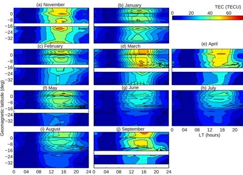
We illustrate the occurrence of the EIA over the region by contour plots of monthly mean TEC as a function of mag-netic latitude and LT. The monthly mean TEC plotted values
[image:4.612.65.268.96.267.2]were obtained from the 19 GNSS receiver stations listed in Table 1. The contour plots helped in determining the loca-tion of the trough and the region of the crest over the East African sector. Figure 2a–j are for the months of November and January–September. The panels for the months of Octo-ber and DecemOcto-ber are missing because these months do not have data over several stations. The data gaps would limit observation of the EIA features over the region. In Fig. 2, the colour bar ranges from blue (low TEC) to red (high TEC). The white spaces within a panel indicate missing data.
(a) November
−32 −24 −16 −8 0
(b) January
(c) February
−32 −24 −16 −8 0
(d) March (e) April
(f) May
Geomagnetic latitude (deg)
−32 −24 −16 −8 0
(g) June (h) July
LT (hours)
0 04 08 12 16 20 24
(i) August
LT (hours)
0 04 08 12 16 20 24
−32 −24 −16 −8 0
(j) September
LT (hours)
0 04 08 12 16 20 24
0 20 40 60 80
[image:5.612.60.540.63.409.2]TEC (TECU)
Figure 2.Contour plots of monthly mean TEC as a function of latitude and LT.(a–j)are for November and January–September.
the magnetic latitude range of 0–4◦S are the strongest com-pared to other latitudes. This implies that over the region, the location where the fountain effect is triggered lies slightly south of the magnetic equator.
In Fig. 2, the southern crest appears to exist from 4 to 19◦S, covering locations of MOIU, EBBE, RCMN, MAL2, ARSH, DODM and TUKC. Among the stations at the trough, ARMI appeared to have more data. Therefore, in our calcula-tion of EIA strengths, the VTEC over ARMI was considered as that of the trough, while the VTEC over other stations with latitudes ranging 8–19.5◦S were considered as VTEC data at the crest. Our results during the high solar activity period of 2011–2013 differ in some aspects from the study done during the low solar activity year of 2009 reported by Bolaji et al. (2017). For instance, their study revealed that the daytime EIA occurrence rarely exceeds 18:00 LT and there was prac-tically no occurrence of the EIA past this time. The highest strength of TEC at the southern crest depicted by their study was about 50 TECU, while our results demonstrated approx-imately 80 TECU. Whereas the inner edge of the southern crest they established was slightly further from the magnetic equator (∼17◦S), our results indicated the same close to the
magnetic equator (4◦S). The increased electron density close to the magnetic equator we observed might be due to ionisa-tion resulting from the locaionisa-tion of the sun above the south-ern crest close to the zenith. Otherwise, during high solar activity conditions the EEJ values are expected to increase. This should have originated from the increased zonal elec-tric field which results in the increased EIA when plasma is transported far from the magnetic equator.
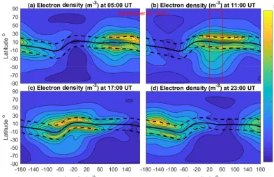
Figure 3.Panels(a),(b),(c)and(d)present the global distribution of electron density derived from the IRI model at 05:00, 11:00, 17:00 and 23:00 UT, respectively on 2 September 2013. The black solid and dotted lines indicate the locations of the magnetic equator and the crests of the EIA. The red box indicates the longitude sector of the current study region.
3.2 EIA morphology depicted by International Reference Ionosphere (IRI) model
For the international standard specification of ionospheric parameters, the Committee On Space Research (COSPAR) and the International Union of Radio Science (URSI) rec-ommended the IRI model. The model is primarily devel-oped using data sources, such as the (i) worldwide net-work of ionosondes and incoherent scatter radars, (ii) ISIS and Alouette topside sounders and (iii) in situ instruments flown on satellites and rockets (http://irimodel.org/, last ac-cess: 1 May 2018). However, theoretical considerations have been used in bridging data gaps and for internal consistency checks (Bilitza, 2001). In order to verify our observations of a southward displacement of the EIA trough, we used global snapshots of the EIA morphology depicted by the IRI 2012 model at an altitude of 100 km. Figure 3a, b, c and d present the distribution of electron density as a function of longi-tude and latilongi-tude at 05:00, 11:00, 17:00 and 23:00 UT, re-spectively on 2 September 2013. The selection of this date aimed at identifying a year and season when high chances of EIA occurrence exist. This particular date considered was geomagnetically quiet since the study only analysed data dur-ing such conditions. It is important to note that we specified the date and geographic coordinates, while the rest of the in-put parameters required by the model were provided by the default option in the model. In Fig. 3, the red box indicates the longitude range 20–60◦, where our region of study lies.
The black solid and dashed lines indicate the location of the magnetic equator and the nominal location of the EIA crests, respectively. The colour bar ranges from blue to yellow, in-dicating low and high electron densities, respectively.
Within the red box in Fig. 3b, it can be seen that the trough is not symmetrical over the magnetic equator. This seems to support our observation of the EIA trough over the East African region being displaced slightly southward. The loca-tion of the EIA trough is symmetrical over longitudes∼100◦ (Fig. 3a) and the range from−80 to−60◦ (Fig. 3c and d), while it is slightly displaced southward over the longitude range from −20 to 20◦ (Fig. 3c) and 20 to 60◦ (Fig. 3b). Figure 3a appears to show that, over India, at a longitude of∼80◦, the EIA trough centre lies south of the magnetic equator. This is in line with the result that over Indian region, the dip latitude of the centre of the EEJ is∼ −0.19◦(Rabiu et al., 2012). More time is needed to check over other longi-tude sectors if the alignment of the EIA trough with respect to the magnetic equator is similar to that of the EEJ. Other-wise, based on the cases observed over Africa and India, we suggest that the location of the EIA trough over a particular longitude depends on the alignment of the centre of the EEJ with respect to the magnetic equator.
9 12 15 18 (a) EEJ
9 12 15 18
(b) CT:TEC ratio (DODM)
9 12 15 18
(c) CT:TEC ratio(MAL2)
9 12 15 18 (d) CT:TEC ratio(MOIU)
LT (hours) −40
−20 0 20 40 60 80 100
0 0.5 1 1.5 2
Jun Jul Aug Sep Oct
Apr
Mar
Feb
[image:7.612.75.522.63.389.2]Jan May Nov Dec
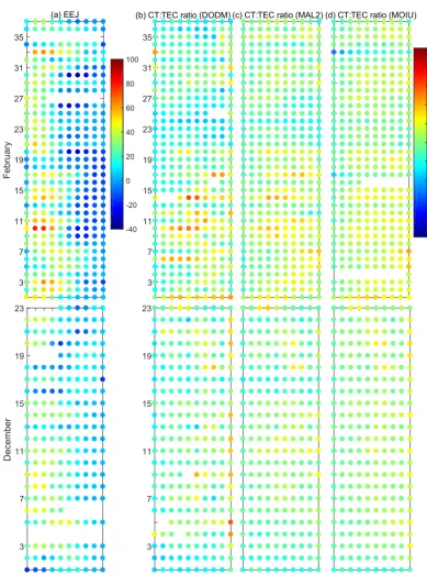
Figure 4.Panel(a)shows variation of the hourly EEJ as a function of LT during days in monthly bins. Corresponding CT : TEC ratios over
DODM, MAL2 and MOIU are shown in(b–d), respectively. Arrows pointing right and left indicate some cases of the prominent EIA during the strong daytime EEJ and the background-level EIA during the weak daytime EEJ, respectively.
3.3 Simultaneous observations of EEJ and EIA strengths
The hourly EIA strengths were used to constitute the daily EIA strengths. The maximum CT : TEC ratio in a 1 h inter-val could be used to represent the EIA strength in that in-terval. Since such values are prone to errors, the upper quar-tile, which is close to the maximum value, was used for such representation. The development of the EIA exhibits a diur-nal pattern that is dependent on the phase of the solar ac-tivity cycle (Rush et al., 1969; Sastri, 1990). At the solar maximum, though the formation of the crests takes place around 09:00 LT, the crests continue to develop and move polewards throughout the day till around 20:00 LT. Based on this idea and the fact that the EEJ is a daytime phenomenon, the local time intervals considered to determine hourly EIA strengths (upper quartile of CT : TEC ratios in a 1 h interval) in a day in this study ranged from 09:00 to 18:00 LT. The daily EIA strengths for the entire study period (2011–2013) were binned according to months, yielding 12 monthly bins. In a similar way, hourly EEJ strengths were also computed
to constitute daily values, which were then binned based on months.
Figure 4 presents the daily EEJ strengths (panel a) and the corresponding EIA strengths over DODM (panel b), MAL2 (panel c) and MOIU (panel d). The horizontal dotted lines separate data of the various monthly bins which are labelled on the vertical axis. The colour bar between panels (a) and (b) ranges from blue (low EEJ) to red (high EEJ). In the case of the colour bar to the right of panel (d), blue denotes a low CT : TEC ratio, while red denotes a high CT : TEC ratio. For the sake of illustration and making sure that the southern crest is well covered, the three stations (DODM, MAL2 and MOIU) are almost separated by about 4◦magnetic latitude and are well distributed over the southern crest.
there are many other factors that may disturb this mecha-nism of EIA formation, which in turn limits observation of the EIA on some days. It can be deduced from Fig. 4b–d that a CT : TEC ratio≥1 signified prominent occurrence of the EIA (TEC over the crest exceeds that over the trough by a factor≥1). By visual inspection of Fig. 4, it is difficult to relate the variations in occurrence of the EIA at background levels (CT : TEC ratio<1) over the stations with that of day-time EEJ strength. However, the conspicuous cases when high EEJ strength (≥50 nT) simultaneously occurs with the prominent EIA are clearly visible over MAL2 and DODM. Some of the cases are marked in Fig. 4, with arrows pointing to the right. The arrows pointing to the left in Fig. 4 depict cases when throughout the day, low values of EEJ (<50 nT) and EIA strengths (CT : TEC ratios<1) are measured simul-taneously.
Figure 5 is a zoom-in of Fig. 4 for the months of February and December. In the figure, the vertical numbers indicate the number of days in the monthly bin. The arrows point-ing left in December and February in Fig. 4 correspond to day 1 of the December bin and day 34 of the February bin in Fig. 5, respectively. The arrow pointing right in February in Fig. 4 corresponds to day 11 of February in Fig. 5. These three examples clearly show that high EEJ strengths occur simultaneously with the prominent EIA. This observation is similar to the one made by Bolaji et al. (2017). Their results showed experimental evidence of how EEJ strength, which is a proxy ofE×Bdrift, mostly controls plasma transporta-tion over low latitudes. Usually, low values ofE×Bdrifts result in poor formation of the EIA (Yizengaw et al., 2014; Olwendo et al., 2015).
[image:8.612.315.540.94.179.2]Three other general observations can be made from Fig. 4. (i) The occurrence of the prominent EIA during daytime was fairly common in equinox seasons (February, March, April, September and October) compared to solstice sea-sons (May, June and July). Along 120◦ longitude, Zhang et al. (2009) made similar observations. They reported that the EIA strength showed a semi-annual variation, with maxi-mum peak values occurring in the equinoctial months. More-over, Sethia et al. (1980) used data measured over India dur-ing the low solar activity year of 1975 to show that EEJ ef-fects on TEC and NmF2 due to the associated zonal elec-tric fields are much more pronounced in the equinoxes than in winter and summer. (ii) The EEJ and EIA strengths are weaker in the June solstice compared to other seasons. This is consistent with the results of Yizengaw et al. (2014). (iii) The highest values of EEJ and EIA strengths appear to occur approximately during 11:00–13:00 and 13:00–18:00 LT, re-spectively. In the next subsection we examine the correlation between the hourly EIA strengths and daytime EEJ strength.
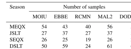
Table 3.Number of samples used to compute correlation
coeffi-cients.
Season Number of samples
MOIU EBBE RCMN MAL2 DODM
MEQX 54 43 40 56 56
JSLT 27 37 27 37 37
SEQX 26 25 19 26 26
DSLT 50 59 24 61 61
3.4 The correlation between daytime EEJ and EIA strengths
In order to determine the correlation between daytime EEJ and EIA strengths, the daily EIA strengths (data similar to that plotted in panels (b)–(d) of Fig. 4) were first binned into the March equinox (March and April), the June solstice (June and July), the September equinox (September and October) and the December solstice (December and January). These seasons were denoted as MEQX, JSLT, SEQX and DSLT, re-spectively. The seasonal bins were further binned according to local time, with a window size of 1 h. The values of EIA strengths at every local time bin were then correlated with the values of the daytime EEJ strength (mean of the EEJ dur-ing the period 10:00–13:00 LT) of the corresponddur-ing days. Figure 6 presents the variation of the correlation coefficients as a function of LT in MEQX (blue), JSLT (green), SEQX (yellow) and DSLT (black). Panels (a)–(e) are for the coef-ficients that were determined over MOIU, EBBE, RCMN, MAL2 and DODM, respectively. These stations lie within the first southern EIA crest and they are among the seven GNSS stations which were used to construct Table 2. Cor-relation coefficients for stations such as ARSH and TUKC were not presented because of insufficient data. Regarding the second southern crest seen in Fig. 2, in addition to sta-tions lying there not having enough data, its occurrence does not seem to be dominant in any of the months.
After filtering the data of days with the afternoon CEJ, un-realistic values of daytime EEJ and EIA strengths, the num-ber of samples over a particular station remained almost con-stant at all LT bins for a specific season. The afternoon CEJ days were identified when the EEJ values remained nega-tive consecunega-tively for≥2 h during 14:00–18:00 LT (Reddy, 1989; Hajra et al., 2009; Rastogi, 1974). Although it still needs to be investigated, we assumed that the morning CEJ might not affect EIA development significantly. The number of samples used to compute the correlation coefficients that are presented in Fig. 6 are shown in Table 3.
9 12 15 18 3
7 11 15 19 23 27 31 35
February
(a) EEJ
-40 -20 0 20 40 60 80 100
9 12 15 18 3
7 11 15 19 23 27 31 35
(b) CT:TEC ratio (DODM)
9 12 15 18 (c) CT:TEC ratio (MAL2)
9 12 15 18 (d) CT:TEC ratio (MOIU)
0 0.2 0.4 0.6 0.8 1 1.2 1.4 1.6 1.8 2
9 12 15 18 3
7 11 15 19 23
December
9 12 15 18 LT (hours) 3
7 11 15 19 23
[image:9.612.104.493.61.583.2]9 12 15 18 9 12 15 18
Figure 5.A zoom-in of Fig. 4 for the months of February and December.
does not vary with LT, yet both cases of significant and non-significantrvalues exist during all the seasons. However, we noted that the cases of non-significantrvalues mostly occur when occurrence of the EIA does not seem to be influenced by the strength of the EEJ (r≤0.3, which occur mostly dur-ing periods<11:00 and>16:00 LT).
Overall, Fig. 6 shows thatr values appear to be positive and increasing from 09:00 up to 13:00 LT when the peak oc-curred and then decreasing gently till 18:00 LT. The averager
activ-−0.3 −0.1 0.1 0.3 0.5 0.7 0.9
(a) MOIU
MEQX JSLT SEQX DSLT
(b) EBBE
−0.3 −0.1 0.1 0.3 0.5 0.7 0.9
(c) RCMN
9 10 11 12 13 14 15 16 17 18
(d) MAL2
LT (hours)
9 10 11 12 13 14 15 16 17 18
−0.3 −0.1 0.1 0.3 0.5 0.7 0.9
(e) DODM
LT (hours)
[image:10.612.102.496.68.342.2]Correlation coefficient, r
Figure 6.The LT variation of correlation coefficients between hourly EIA strength and daytime EEJ strength in MEQX (blue), JSLT (green),
SEQX (yellow) and DSLT (black). Panels(a–e)are for correlation coefficients over MOIU, EBBE, RCMN, MAL2 and DODM, respectively.
ity year of 1958, the correlation coefficients between the EIA and EEJ parameters maximised during 13:00–15:00 LT. The unique feature presented by Fig. 6 is the strong positive cor-relations in SEQX over MAL2 and DODM that remained till 18:00 LT. This point needs further investigation. However, it can be noted that these two stations are far from the magnetic equator compared to the remaining three. Moreover, they are closer to the nominal southern crest of the EIA at 15◦S.
Based on the general trend, the occurrence of strong posi-tive correlations during 13:00–15:00 LT between the EIA and the daytime EEJ strength is consistent with the idea that the EIA maximises about a few (2–4) hours from the time of the intensified cause. In this case, the cause might be the in-creased zonal electric field manifested in the EEJ that ap-peared to peak during 11:00–13:00 LT (see Fig. 4). There is no clear trend in thervalues that are related to the seasonal and latitudinal variations. There might be an average value of daytime EEJ strength above which chances of prominent zonal electric field and EIA occurrence might be high. In the next subsection, we illustrate how such a value can be deter-mined.
3.5 A threshold EEJ strength
As deduced from Fig. 4, cases of daytime prominent EIA might be associated with the EEJ≥50 nT. The approximate values for each station considered in this study were
deter-Table 4.Percentage of prominent EIA corresponding to threshold
EEJ strength.
Season, LT Station
MOIU EBBE RCMN MAL2 DODM
MEQX, 13:00 97 80 86 94 43
SEQX, 13:00 91 81 60 100 45
DSLT, 13:00 100 95 100 100 95
MEQX, 14:00 100 83 86 86 50
SEQX, 14:00 100 90 80 91 64
DSLT, 14:00 100 100 100 100 90
MEQX, 15:00 97 87 82 86 56
SEQX, 15:00 91 73 80 82 73
DSLT, 15:00 95 100 100 86 95
[image:10.612.308.551.432.568.2]0 2 4 6
(a) EEJ distribution (MOIU)
No. of observations
0 2 4 6
(b) EEJ distribution (EBBE)
0 2 4 6
(c) EEJ distribution (RCMN)
0 2 4 6
(d) EEJ distribution (MAL2)
< 20 20−25 25−30 30−35 35−40 40−45 45−50 50−55 55−60 60−65 65−70 > 70
0 2 4 6
(e) EEJ distribution (DODM)
EEJ (nT)
Tot = 11, mean = 44.2 nT, SD = 9.9 nT
Tot = 6, mean = 59.8 nT, SD = 9.9 nT
Tot = 12, mean = 54.8 nT, SD = 17.4 nT
Tot = 18, mean = 55.6 nT, SD = 15.8 nT
[image:11.612.103.494.68.345.2]Tot = 17, mean = 60.9 nT, SD = 19.2 nT
Figure 7.The distributions of EEJ strengths associated with prominent EIA at 14:00 LT over(a)MOIU,(b)EBBE,(c)RCMN,(d)MAL2,
and(e)DODM.
right of each panel, the total number (Tot), mean and standard deviation (SD) of the EEJ values are indicated. It can be ob-served from the panels that the mean EEJ at which the promi-nent EIA occurred ranged from 44.2 to 60.9 nT (overall mean 55.1 nT), while the SD ranged from 9.9 to 19.2 nT (overall SD 14.4 nT). Therefore, over the East African sector, the EIA might occur prominently during 13:00–15:00 LT when mea-surements of the EEJ≥40.7 nT (overall mean EEJ−overall SD) are made.
The suitability of the EEJ threshold value (40.7 nT) to pre-dict occurrence of the EIA was ascertained. This was again done for MEQX, SEQX and DSLT when high chances of prominent EIA occurrence were expected. The number of observed EIA occurrences (CT : TEC ratio>1) during days with EEJ strength ≥40.7 nT were determined for each sea-son and station. These were denoted as NoPromEIA. The total number of observed EIA strengths (including both a CT : TEC ratio ≤1 and a CT : TEC ratio >1) during days with EEJ strength ≥40.7 nT were also determined and de-noted as TotalNoEIA. The ratios of NoPromEIA to To-talNoEIA were expressed as percentages. Table 4 presents the percentages that were determined over MOIU, EBBE, RCMN, MAL2 and DODM. In the table, column 1 presents the seasons and the three local times 13:00, 14:00 and 15:00 at which the percentages were determined. At 13:00, 14:00 and 15:00 LT, the fractions of the number of entries with
per-centages >80 were 12/15, 13/15 and 12/15, respectively. Therefore, the percentages at the three local times (13:00, 14:00 and 15:00 LT) were similar. These fractions indeed confirm the fact that the chances of observing prominent EIA occurrence are high when measurements of EEJ strength of at least 40.7 nT are made. This appears to be the first time that a threshold value of the EEJ over the East African region has been determined that can be associated with the zonal electric field, which in turn produces the pronounced EIA.
4 Conclusions
re-gion are consistent with those reported over other rere-gions by the previous studies, the next two results appear to be novel. (iv) Over the East African region, the trough of the EIA during high solar activity and quiet geomagnetic con-ditions lies slightly south (0–4◦S) of the magnetic equator. We suggest that the slight southward shift of the EIA trough is consistent with the general centre of the EEJ. The latter is also shifted slightly south of the magnetic equator. (v) Dur-ing the equinox and December solstice seasons, and the local time interval of 13:00–15:00, the probability of observing the EIA on days with daytime EEJ strength≥40 nT was mostly
>80 %. It should be noted that these results pertain to a high solar activity period in the ascending phase of Solar Cycle 24. They might change in the seasons of a solar minimum period. This was not done due to unavailability of geomagnetic field measurements over the East African region.
Data availability. The data used in this study were ob-tained from ftp://data-out.unavco.org/pub/rinex/, http: //swdcwww.kugi.kyoto-u.ac.jp/, http://www.intermagnet.org, last access: 15 September 2015, http://magnetometers.bc.edu, last access: 15 September 2017 and http://spidr.ionosonde.net/spidr/, last access: 1 May 2018.
Competing interests. The authors declare that they have no conflict of interest.
Acknowledgements. Patrick Mungufeni is thankful to his scien-tific coordinator at the Abdus Salam International Centre for Theo-retical Physics (ICTP), Sandro Radicella. Through the associate-ship scheme with ICTP and with the help of Sandro Radicella, Patrick Mungufeni attended many workshops/conferences organ-ised by ICTP in the research field of this manuscript. The knowl-edge obtained during the workshops and the interaction with other scientists helped in formulating the problem presented in this study. John Bosco Habarulema’s contributions were supported by the South African National Research Foundation (NRF) grant 105778. The International Science Programme of Sweden supported the contributions of Edward Jurua.
The topical editor, Dalia Buresova, thanks two anonymous ref-erees for help in evaluating this paper.
References
Abdu, M. A.: The International Equatorial Electro-jet Year, AGU, EOS transactions, 73, 49–64, 1992.
Anderson, D., Anghel, A., Yumoto, K., Ishitsuka, M., and Kudeki, E.: Estimating daytime vertical E×B drift veloc-ities in the equatorial F-region using ground-based magne-tometer observations, Geophys. Res. Lett., 29, 12, 37-1–37-4 https://doi.org/10.1029/2001GL014562, 2002.
Anderson, D., Anghel, A., Chau, J., and Veliz, O.: Daytime ver-tical E×B drift velocities inferred from ground-based
mag-netometer observations at low latitudes, Space Weather, 2, https://doi.org/10.1029/2004SW000095, 2004.
Appleton, E. V.: Two Anomalies in the Ionosphere, Nature, 691, 1946.
Bilitza, D.: International Reference Ionosphere 2000, Radio Sci., 36, 261–276, 2001.
Bolaji, O., Owolabi, O., Falayi, E., Jimoh, E., Kotoye, A., Odeyemi, O., Rabiu, B., Doherty, P., Yizengaw, E., Yamazaki, Y., Adeniyi, J., Kaka, R., and Onanuga, K.: Observations of equatorial ionization anomaly over Africa and Middle East dur-ing a year of deep minimum, Ann. Geophys., 35, 123–132, https://doi.org/10.5194/angeo-35-123-2017, 2017.
Chakraborty, S. K. and Hajra, R.: Electrojet control of ambient ion-ization near the crest of the equatorial anomaly in the Indian zone, Ann. Geophys., 27, 93–105, https://doi.org/10.5194/angeo-27-93-2009, 2009.
Chapman, S.: The equatorial electro-jet as detected from the ab-normal electric current distribution about Huancayo, Peru and elsewhere, Arch. Meteor. Geophy. A, 4, 368–390, 1951. Gouin, P.: Reversal of the magnetic daily variation at Addis Ababa,
Nature, 193, 1145–1146, 1962.
Gouin, P. and Mayaud, P. N.: A propos de lexistence possible d’un “contre-electrojet” aux latitudes magnetiques equatoriales, Ann. Geophys., 23, 41–47, 1967.
Hajra, R., Chakraborty, S. K., and Paul, A.: Electro-dynamical con-trol of the ambient ionization near the equatorial anomaly crest in the Indian zone during counter electrojet days, Radio Sci., 44, RS3009, https://doi.org/10.1029/2008RS003904, 2009. Kane, R. P. and Rastogi, R. G.: Some Characteristics of the
Equa-torial Electrojet in Ethiopia (East Africa), Indian J. Radio Space, 6, 85–101, 1977.
Kane, R. P. and Trivedi, N. B.: Are the equatorial electrojet and counterelectrojet centered invariably on the dip equator, J. At-mos. Terr. Phys., 44, 301–304, 1982.
Mungufeni, P., Habarulema, J. B., and Jurua, E.: Modeling of Iono-spheric Irregularities during Geomagnetically Disturbed Condi-tions over African Low Latitude Region, Space Weather, 710– 723, https://doi.org/10.1002/2016SW001446, 2016.
Olwendo, O. J., Yosuke, Y., Pierre, C., Baki, P., Ngwira, C. M., and Mito, C.: A study on the response of the Equatorial Ioniza-tion Anomaly over the East Africa sector during the geomagnetic storm of November 13, 2012, Adv. Space Res., 55, 2863–2872, https://doi.org/10.1016/j.asr.2015.03.011, 2015.
Rabiu, A. B., Onwumechili, C. A., Nagarajan, N., and Yumoto, K.: Characteristics of equatorial electrojet over India determined from a thick current shell model, J. Atmos. Sol.-Terr. Phy., 92, 105–115, 2012.
Rastogi, R. G.: Westward Equatorial Electro-jet During Daytime Hours, J. Geophys. Res., 79, 1503–1512, 1974.
Reddy, C. A.: The Equatorial Electro-jet, PAGEOPH, 131, 485– 508, 1989.
Rodriguez-Zuluaga, J., Radicella, M., S., Nava, B., Amory-Mazaudier, C., Mora-Páez, H., and Alazo-Cuartas, K.: Distinct responses of the low-latitude ionosphere to CME and HSSWS: The role of the IMF Bz oscillation frequency, J. Geophys. Res.-Space Phys., 121, 11528–11548, 2016.
Rush, C. M., Rush, S. V., Lyons, L. R., and Venkateswaran, S. V.: Equatorial anomaly during a period of declining solar activity, Radio Sci., 4, 829–841, 1969.
Sastri, J. H.: Post-Sunset Behaviour of the Equatorial Anomaly in the Indian Sector, Indian J. Radio Space, 11, 33–37, 1982. Sastri, J. H.: Equatorial anomaly in F-region – A review, Indian J.
Radio Space, 19, 225–240, 1990.
Seemala, G. and Valladares, C.: Statistics of total elec-tron content depletions observed over the South Ameri-can continent for the year 2008, Radio Sci., 46, RS5019, https://doi.org/10.1029/2011RS004722, 2011.
Sethia, G., Rastogi, R. G., Deshpande, M. R., and Chandra, H.: Equatorial Electrojet Control of the Low Latitude Ionosphere, J. Geomagn. Geoelectr., 32, 207–216, 1980.
Subhadra Devi, P. K. and Unnikrishnan, K.: Study of daytime ver-ticalE×Bdrift velocities inferred from ground-based magne-tometer observations of1H, at low latitudes under geomagneti-cally disturbed conditions, Adv. Space Res., 53, 752–762, 2014. Venkatesh, K., P. R., Fagundes, D. S. V. V. D., Prasad, C. M., Denar-dini, A. J., de Abreu, R. D. J., and Gende, M.: Day-to-day vari-ability of equatorial electro-jet and its role on the day-to-day characteristics of the equatorial ionization anomaly over the In-dian and Brazilian sectors, J. Geophys. Res.-Space Phys., 120, 9117–9131, https://doi.org/10.1002/2015JA021307, 2015.
Yizengaw, E., Moldwin, M. B., Mebrahtu, A., Damtie, B., Zesta, E., Valladares, C. E., and Doherty, P.: Comparison of storm time equatorial ionospheric electrodynamics in the African and Amer-ican sectors, J. Atmos. Sol.-Terr. Phy., 73, 156–163, 2010. Yizengaw, E., Moldwin, M. B., Zesta, E., Biouele, C. M., Damtie,
B., Mebrahtu, A., Rabiu, B., Valladares, C. F., and Stoneback, R.: The longitudinal variability of equatorial electrojet and verti-cal drift velocity in the African and American sectors, Ann. Geo-phys., 32, 231–238, https://doi.org/10.5194/angeo-32-231-2014, 2014.
Yue, X., Schreiner, W., Kuo, Y., and Lei, J.: Ionosphere equatorial ionization anomaly observed by GPS radio occultations during 2006–2014, J. Atmos. Sol.-Terr. Phy., 129, 30–40, 2015. Zhang, M.-L., Wan, W., Liu, L., and Ning, B.: Variability study