DOI:10.1051/0004-6361/201731403 c
ESO 2017
Astronomy
&
Astrophysics
Variable millimetre radiation from the colliding-wind binary
Cygnus OB2 #8A
?
R. Blomme
1, D. M. Fenech
2, R. K. Prinja
2, J. M. Pittard
3, and J. C. Morford
21 Royal Observatory of Belgium, Ringlaan 3, 1180 Brussels, Belgium
e-mail:[email protected]
2 Department of Physics and Astronomy, University College London, Gower Street, London WC1E 6BT, UK 3 School of Physics & Astronomy, E.C. Stoner Building, The University of Leeds, Leeds LS2 9JT, UK
Received 19 June 2017/Accepted 14 August 2017
ABSTRACT
Context.Massive binaries have stellar winds that collide. In the colliding-wind region, various physically interesting processes occur, leading to enhanced X-ray emission, non-thermal radio emission, as well as non-thermal X-rays and gamma-rays. Non-thermal radio emission (due to synchrotron radiation) has so far been observed at centimetre wavelengths. At millimetre wavelengths, the stellar winds and the colliding-wind region emit more thermal free-free radiation, and it is expected that any non-thermal contribution will be difficult or impossible to detect.
Aims.We aim to determine if the material in the colliding-wind region contributes substantially to the observed millimetre fluxes of a colliding-wind binary. We also try to distinguish the synchrotron emission from the free-free emission.
Methods.We monitored the massive binary Cyg OB2 #8A at 3 mm with the NOrthern Extended Millimeter Array (NOEMA) inter-ferometer of the Institut de Radioastronomie Millimétrique (IRAM). The data were collected in 14 separate observing runs (in 2014 and 2016), and provide good coverage of the orbital period.
Results.The observed millimetre fluxes range between 1.1 and 2.3 mJy, and show phase-locked variability, clearly indicating that a large part of the emission is due to the colliding-wind region. A simple synchrotron model gives fluxes with the correct order of magnitude, but with a maximum that is phase-shifted with respect to the observations. Qualitatively this phase shift can be explained by our neglect of orbital motion on the shape of the colliding-wind region. A model using only free-free emission results in only a slightly worse explanation of the observations. Additionally, on the map of our observations we also detect the O6.5 III star Cyg OB2 #8B, for which we determine a 3 mm flux of 0.21±0.033 mJy.
Conclusions.The question of whether synchrotron radiation or free-free emission dominates the millimetre fluxes of Cyg OB2 #8A remains open. More detailed modelling of this system, based on solving the hydrodynamical equations, is required to give a definite answer.
Key words. binaries: spectroscopic – stars: winds, outflows – stars: individual: Cyg OB2 #8A – stars: individual: Cyg OB2 #8B – stars: massive – radio continuum: stars
1. Introduction
Massive stars have strong stellar winds. When two such stars form a binary, their stellar winds collide, leading to a number of interesting effects. The collision between the two winds heats up the material to such temperatures that it emits detectable X-ray radiation, as originally predicted by Prilutskii & Usov (1976) and recently reviewed by Rauw & Nazé(2016). In the shocks associated with the colliding-wind region (CWR), a fraction of the electrons are accelerated to high, non-thermal energies by the Fermi mechanism (Bell 1978; Eichler & Usov 1993). These electrons spiral in the magnetic field, thereby emitting synchrotron emission, which we can detect as non-thermal ra-dio emission (Bieging et al. 1989).
In an eccentric binary, the strength of the collision (more specifically, the ram pressure) will vary with orbital phase, lead-ing to phase-locked variations of the intrinsic emission com-ing from the CWR. At radio wavelengths, there is furthermore ? This work is based on observations carried out under project
num-bers S14AW and S16AU with the IRAM NOEMA Interferometer. IRAM is supported by INSU/CNRS (France), MPG (Germany) and IGN (Spain).
the effect of the strong free-free absorption in the stellar wind material (Wright & Barlow 1975). The changing positions of both stellar winds and the CWR lead to further phase-locked variations in the observed radio fluxes. This has been observed in a number of O+O and Wolf-Rayet+O colliding-wind bi-naries (e.g., White & Becker 1995; Blomme et al. 2005, 2007; Blomme & Volpi 2014). In exceptional cases, the CWR has been resolved by high-resolution radio observations (Benaglia et al. 2015, and references therein).
Colliding winds also emit non-thermal X-rays and gamma-rays (Pollock 1987; Benaglia & Romero 2003; Pittard et al. 2006; Reimer et al. 2006; De Becker 2007; Reitberger et al. 2014), making these objects very relevant to high-energy physics (Pittard & Dougherty 2006). The regime of physical parame-ters (density, magnetic field, ambient radiation field, etc.) is quite different from that of other high-energy environments, and colliding-wind binaries can therefore provide important tests of our understanding of the physical processes responsible.
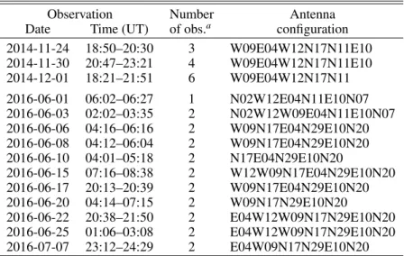
Table 1.Observing log of the NOEMA 3 mm observations of Cyg OB2 #8A.
Observation Number Antenna
Date Time (UT) of obs.a configuration 2014-11-24 18:50–20:30 3 W09E04W12N17N11E10 2014-11-30 20:47–23:21 4 W09E04W12N17N11E10 2014-12-01 18:21–21:51 6 W09E04W12N17N11 2016-06-01 06:02–06:27 1 N02W12E04N11E10N07 2016-06-03 02:02–03:35 2 N02W12W09E04N11E10N07 2016-06-06 04:16–06:16 2 W09N17E04N29E10N20 2016-06-08 04:12–06:04 2 W09N17E04N29E10N20 2016-06-10 04:01–05:18 2 N17E04N29E10N20
2016-06-15 07:16–08:38 2 W12W09N17E04N29E10N20 2016-06-17 20:13–20:39 2 W09N17E04N29E10N20 2016-06-20 04:14–07:15 2 W09N17N29E10N20
2016-06-22 20:38–21:50 2 E04W12W09N17N29E10N20 2016-06-25 01:06–03:08 2 E04W12W09N17N29E10N20 2016-07-07 23:12–24:29 2 E04W09N17N29E10N20
Notes.(a)A single observation on Cyg OB2 #8A consists of 30 or 33 scans (for the 2014 and 2016 runs, respectively), where each scan is 45 s.
clumping decreases the mass loss rates by a factor 3–10 com-pared to what was previously thought (e.g., Puls et al. 2008). This, in turn, has major consequences for stellar and galactic evolution. Colliding-wind systems can provide an independent determination of the effect of clumping and porosity (e.g.,Pittard 2007): by modelling the colliding winds, and predicting the vari-ous observational indicators, we can constrain the mass-loss rate and/or porosity in the wind.
Colliding-wind binaries have so far been relatively unplored at millimetre wavelengths. This is mainly due to the ex-pectation that free-free emission will start to dominate the fluxes at shorter wavelength, and that therefore the non-thermal syn-chrotron emission will be difficult or impossible to detect.
Furthermore, the CWR will also increase the free-free emis-sion, as shown byStevens(1995) andMontes et al.(2011), using simplified models for a radiative shock; and byDougherty et al. (2003),Pittard et al.(2006) and Pittard(2010), using hydrody-namical calculations for both adiabatic and radiative shocks. The density increase leads to a considerable amount of additional free-free emission. Montes et al.(2015) tried to look for this, by comparing centimetre and millimetre fluxes for a sample of 17 Wolf-Rayet stars. For three of these, a hint from the colliding-wind region contribution was found, but their observations did not allow to clearly identify the physical mechanism.
Another approach is to look for the variability of the millime-tre fluxes. An eccentric binary will show phase-locked variabil-ity of the millimetre fluxes for the same reason as for the radio fluxes. The changing distance between the two components leads to variation in the strength of the collision and hence the amount of additional free-free emission. Added to that is the variation in the free-free absorption due to the changing position of the stellar winds and the CWR.
Cyg OB2 #8A (=Schulte 8A=MT 465=BD+40 4227A) is a well-known massive colliding-wind binary, and therefore an appropriate candidate to look for variability at millimetre wavelengths. It is a member of Cyg OB2, which is an associ-ation containing a large number of massive stars (Knödlseder 2000;Wright et al. 2015). The association harbours a number of massive colliding-wind binaries that have been studied in detail (Van Loo et al. 2008;Blomme et al. 2010,2013;Kennedy et al. 2010).
Cyg OB2 #8A was discovered to be a binary by De Becker et al.(2004). It has a period P=21.908±0.040 d, an eccentricitye=0.24 ±0.04, and it consists of an O6If pri-mary and an O5.5III(f) secondary (De Becker et al. 2006). It has all the attributes of a colliding-wind binary. Its radio spectrum shows a negative spectral index (Bieging et al. 1989) and the ra-dio flux variations are locked to the orbital phase (Blomme et al. 2010). The X-ray emission is overluminous compared to that of single O-type stars and its variability is also phase-locked (De Becker et al. 2006;Blomme et al. 2010). Among the O-type colliding-wind binaries, it is the system where the parameters of the stars, their stellar wind and their orbit are best known (De Becker 2007).
We observed Cyg OB2 #8A with the NOrthern Extended Millimeter Array (NOEMA) interferometer of the Institut de Ra-dioastronomie Millimétrique (IRAM1), to see if we could de-tect the expected flux variations at millimetre wavelengths. We present the observations in Sect. 2 and the data reduction in Sect.3. The resulting millimetre light curve is given in Sect.4 and we model it in Sect.5. In Sect.6, we present the results for Cyg OB2 #8B, which is the visual companion to our main target. The conclusions are given in Sect.7.
2. Observations
Cyg OB2 #8A was observed with the IRAM NOEMA inter-ferometer during two different periods: end of 2014 (project: S14AW; PI: D.M. Fenech) and mid-2016 (project S16AU; PI: R. Blomme). The 2014 observations consist of three runs (a fourth run, on 2014-11-29, contains only calibrator data and no on-target observations, so it will not be considered further). The 2016 observations have 11 runs. The detailed observing log is given in Table1.
Observations were collected at 3 mm (110 GHz; IRAM re-ceiver no. 1 in Upper Side Band), in single-pointing mode. Dual polarization was used with a bandwidth of 2×3.6 GHz. An ob-serving run consists of alternating between one or two phase cal-ibrators and Cyg OB2 #8A, ensuring that each Cyg OB2 #8A observation is preceded and succeeded by a phase calibrator ob-servation. In addition, for each run, the flux calibrator MWC 349
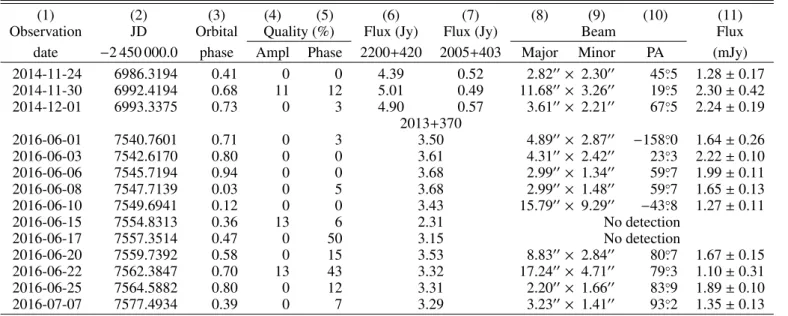
Table 2.Measured 3 mm fluxes of Cyg OB2 #8A.
(1) (2) (3) (4) (5) (6) (7) (8) (9) (10) (11)
Observation JD Orbital Quality (%) Flux (Jy) Flux (Jy) Beam Flux
date −2 450 000.0 phase Ampl Phase 2200+420 2005+403 Major Minor PA (mJy)
2014-11-24 6986.3194 0.41 0 0 4.39 0.52 2.8200× 2.3000 45◦.5 1.28±0.17
2014-11-30 6992.4194 0.68 11 12 5.01 0.49 11.6800× 3.2600 19◦.5 2.30±0.42
2014-12-01 6993.3375 0.73 0 3 4.90 0.57 3.6100× 2.2100 67◦.5 2.24±0.19
2013+370
2016-06-01 7540.7601 0.71 0 3 3.50 4.8900× 2.8700 −158◦.0 1.64±0.26
2016-06-03 7542.6170 0.80 0 0 3.61 4.3100× 2.4200 23◦.3 2.22±0.10
2016-06-06 7545.7194 0.94 0 0 3.68 2.9900× 1.3400 59◦.7 1.99±0.11
2016-06-08 7547.7139 0.03 0 5 3.68 2.9900× 1.4800 59◦.7 1.65±0.13
2016-06-10 7549.6941 0.12 0 0 3.43 15.7900× 9.2900 −43◦.8 1.27±0.11
2016-06-15 7554.8313 0.36 13 6 2.31 No detection
2016-06-17 7557.3514 0.47 0 50 3.15 No detection
2016-06-20 7559.7392 0.58 0 15 3.53 8.8300× 2.8400 80◦.7 1.67±0.15
2016-06-22 7562.3847 0.70 13 43 3.32 17.2400× 4.7100 79◦.3 1.10±0.31
2016-06-25 7564.5882 0.80 0 12 3.31 2.2000× 1.6600 83◦.9 1.89±0.10
2016-07-07 7577.4934 0.39 0 7 3.29 3.2300× 1.4100 93◦.2 1.35±0.13
Notes.Column (1) gives the date of the observation; Col. (2) the Julian date of the mid-point of the observation; Col. (3) the phase in the 21.908 d orbital period; Cols. (4) and (5) the percentage of data that were flagged because of high amplitude loss and high phase loss, respectively; Cols. (6) and (7) the fluxes of the phase calibrators (only one calibrator for the 2016 data); Cols. (8)–(10) the synthesized beam (major axis×minor axis and position angle PA); Col. (11) the flux of Cyg OB2 #8A, and its error bar.
and the bandpass calibrator 3C 454.3 were observed (for the 2016-06-22 observation the bandpass calibrator 3C 273 was also observed).
During the 2014 runs, the two phase calibrators used were 2200+420 (at an angular distance ∆ = 16◦.7) and 2005+403 (∆ = 4◦.9); in 2016, only 2013+370 (∆ =5◦.4) was used. A sin-gle Cyg OB2 #8A observation consists of 30 scans (33 scans in 2016) of 45 s each. For each phase calibrator observation, three 45 s scans were done. The signals from the antennas were corre-lated with the WideX correlator. During the 2014 observations, the antennas were in the 6Cq configuration (with E10 missing for the 2014-12-01 run). For the 2016 observations, many changes in antenna positions were made; we therefore list the detailed configurations in Table1.
3. Data reduction
We used the GILDAS2software for the data reduction, specif-ically the packages CLIC (for calibration) and MAPPING (for the flux determination).
We split the observing runs, so that we can separately cal-ibrate each series of 30 (or 33 scans) on Cyg OB2 #8A. The phase calibrator(s) immediately preceding and following the Cyg OB2 #8A observations were selected, as well as the band-pass and flux calibrators that are nearest in time. Based on the pipeline reduction that had run at IRAM, we flagged some data which were clearly discrepant, or were on one side of a cable phase jump, or had high system temperatures. The 2014 obser-vations were done in a stable configuration, and therefore needed no baseline corrections. Antenna movement was frequent how-ever during the 2016 observations, and for all these runs, base-line corrections (provided by IRAM staff) were applied.
Default automatic flagging was applied, which flags prob-lems with antenna shadowing, data that do not have surround-ing calibrator observations, and timsurround-ing errors. Next, atmospheric phase corrections were applied. The receiver bandpass was then
2 http://www.iram.fr/IRAMFR/GILDAS/
calibrated on the bandpass calibrator 3C 454.3, using the default degree of the polynomials. For the 2016-06-22 observations, the 3C 454.3 data were not usable, and the bandpass was calibrated on 3C 273. Phase calibration consists of fitting a per-antenna lin-ear function to the phases of the phase calibrator(s). Fluxes were then calibrated on the flux calibrator MWC 349, which has a flux of 1.23 Jy. For the amplitude calibration, a per-antenna lin-ear function was fitted to the calibrators.
As the final part of the calibration, the Data Quality Assess-ment procedure was run. This flags data with more than 40◦ root-mean-square (rms) of phase loss, and more than 20% of ampli-tude loss. The fraction of points that were flagged in this way are indicated in Table2. They are a good indicator of the quality of the data, in the sense that a higher fraction of flagged points in-dicates worse quality. Pointing, focus and tracking errors which are too high are also flagged, but this did not occur for any of our observations. Finally, the calibrated data of Cyg OB2 #8A were written out. At this stage, all Cyg OB2 #8A data taken during a single observing run were merged again.
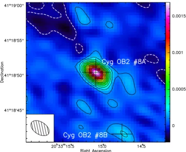
Next, we made a deep image by combining all the data (Fig.1), to see if there are any other sources in the field besides Cyg OB2 #8A. We used a pixel size of 0.400 ×0.400, which is about one-quarter (linear dimension) of the synthesized beam size. We took a grid size of 256 ×256 pixels, which covers somewhat more than twice the primary beam and we applied natural weighting. We then cleaned the image, stopping when we reached 0.025 mJy, which is half of the rms noise level in the image. Figure1shows only the inner 2000×2000part of this image.
The field is dominated by Cyg OB2 #8A, which is – as ex-pected – a point source. A much weaker source is seen at the bottom edge of Fig.1. We identify it as Cyg OB2 #8B, and dis-cuss it further in Sect.6. We checked the full image for other possible sources, but found none.
Fig. 1.Deep 3 mm image of all Cyg OB2 #8A data combined. The colour scale values are in Jy. The contour levels are at −0.1 mJy, +0.1 mJy and then go up in steps of 0.1 mJy to 1.6 mJy. The negative contour is indicated by the dashed, white line. The crosses indicate the positions of Cyg OB2 #8A and #8B (from SIMBAD). The synthesized beam (shown in the lower left corner) is 2.9300×
1.7600
with a position angle of 57◦.
1.
-0.2 0.0 0.2 0.4 0.6 0.8 1.0 1.2
orbital phase
0.0 0.5 1.0 1.5
6 cm flux (mJy)
0.0 0.5 1.0 1.5 2.0 2.5 3.0
3 mm flux (mJy)
Fig. 2.Observed 3 mm fluxes of Cyg OB2 #8A, plotted as a function of orbital phase in the 21.908-day binary period. The blue symbols show the 2014 data, the red ones the 2016 data. To better show the behaviour of the light curve, the phase range is extended by 0.2 on each side. Open symbols indicate duplications in that extended range. The grey data show the 6 cm observations fromBlomme et al.(2010). Note that the 3 mm flux scale (left) is different from the 6 cm one (right).
approach than measuring the flux on images made from these visibilities, as the cleaning procedure might introduce artefacts. The fluxes we obtained are listed in Table2.
A number of variant reductions were also tried: switching off the atmospheric phase correction, using weights in the phase or amplitude calibration, or averaging the polarizations in these cal-ibrations, or flagging frequency parasites (i.e., sharp peaks in fre-quency caused by the instrument). These all gave values within the listed error bars. As the Cyg OB2 #8A flux is relatively high, we also tried to include it in the calibration process, but this did not improve results.
4. Millimetre light curve
The Cyg OB2 #8A fluxes listed in Table2clearly indicate vari-ability. To check that this is not some artefact of the data reduc-tion, we also list the fluxes of the phase calibrators. The phase calibrators are intrinsically variable, and their measured fluxes are clearly not correlated with the Cyg OB2 #8A ones. We can therefore exclude data reduction artefacts. The absolute flux cal-ibration at 3 mm is good to about 10% (J. M. Winters, pers. comm.), which corresponds to about ±0.2 mJy. The flux vari-ations are therefore also not due to changes in the levels of the absolute flux calibration.
We next plot the observed fluxes in the orbital phase dia-gram (Fig.2). The fluxes are clearly correlated with the orbital phase, indicating that they are at least partly formed in the CWR. Around phase 0.7, there is a large range in the fluxes, which seems to violate the assumption that, in a colliding-wind binary, the fluxes repeat nearly perfectly from one orbit to another. We note, however, that the two extreme fluxes are of lower quality: the amplitude quality indicator in Table2shows that 11 and 13% of the data for these two observations have been removed by the Data Quality Assessment procedure, because they show more than 20% amplitude loss. Note that the standard error bar does not include this systematic effect. On the basis of this quality in-formation, we consider the flux variations around phase 0.7 to be not significant.
Figure2also shows the 6 cm radio fluxes fromBlomme et al. (2010). Note that different flux scales are used for the 3 mm and the 6 cm data. The shape of the 3 mm light curve follows that of the 6 cm one very well, but differs from it in two aspects. First, the millimetre data are above the median (1.66 mJy) about 30% of the time, while the 6 cm data are above their median about 50% of the time. This is due to the non-uniform distribution of the phases for which we have flux determinations. There are a large number of observations around the phase of maximum flux (0.7–0.8), but none around the suspected minimum (phase 0.2– 0.3). Additional data around the minimum would lower the me-dian and lead to a more equal distribution of the phase range above and below the median.
Secondly, the 3 mm light curve is phase-shifted with respect to the 6 cm one. One could consider that the uncertainty in the period is responsible for this shift. The 21.908±0.040 d pe-riod was derived byDe Becker et al.(2004) on the basis of spec-troscopic data from the years 2000–2003. However, both X-ray data covering the years 1991–2004 and radio data covering the years 1980–2005 are consistent with this period, suggesting that the 0.040 d error bar is too conservative (De Becker et al. 2006; Blomme et al. 2010). We therefore consider it unlikely that the phase shift is due to uncertainty in the period.
Alternatively, we note that a phase shift in the radio light curves at different wavelengths is quite common for colliding-wind binaries. The most detailed example is WR 140, as shown byWhite & Becker(1995). Specifically for Cyg OB2 #8A, a hint of such a phase shift is present in Fig. 1 ofBlomme et al.(2010). It can be seen when comparing the position of minimum for the 6 cm and 3.6 cm radio observations.
5. Modelling
Table 3.Overview of models used in Sect.5.
Section Model
5.1 Spherically symmetric wind; thermal wind emission only
5.2 Detailed synchrotron emission model; no increased temperature of CWR material; thermal wind emission 5.3 Increased temperature of CWR material; adiabatic shock; no synchrotron emission; thermal wind emission 5.4 Increased temperature of CWR material; radiative shock; no synchrotron emission; thermal wind emission 5.5 Detailed synchrotron emission model; increased temperature of CWR material; thermal wind emission
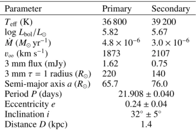
Table 4.Cyg OB2 #8A parameters used in modelling.
Parameter Primary Secondary
Teff(K) 36 800 39 200
logLbol/L 5.82 5.67
˙
M(Myr−1) 4.8×10⁻⁶ 3.0×10⁻⁶
3∞(km s−1) 1873 2107
3 mm flux (mJy) 1.62 0.75
3 mmτ=1 radius (R) 220 140 Semi-major axisa(R) 65.7 76.0 PeriodP(days) 21.908±0.040 Eccentricitye 0.24±0.04
Inclinationi 32◦±5◦
DistanceD(kpc) 1.4
Notes. The parameters were derived byDe Becker et al.(2006). The predicted fluxes and the radii where the optical depthτbecomes 1 for 3 mm (Rτ=1) have been derived from theWright & Barlow(1975)
equa-tions (see Sect.5.1) The values listed do not include clumping. When including clumping, the flux scales as ( ˙Mpfcl)4/3 andRτ=1scales
dif-ferently as ( ˙Mpfcl)2/3, where fclis the clumping factor. Note, however,
that when comparing a clumped wind and a smooth wind that have the same flux, their ˙Mpfclneeds to be the same, hence also theirRτ=1.
5.1. Stellar wind contribution
We first estimate how much the two stellar winds contribute to the observed millimetre fluxes. As a first approximation, we ap-ply the Wright & Barlow(1975) formalism. The expected flux Sν(in mJy) at frequency ν(in Hz) of a spherically symmetric, steady-state wind, with a mass-loss rate ˙M(inMyr−1) flowing out at a constant velocity3∞(in km s−1) is:
Sν=23.2×10³
˙ M
µ3∞
!4/3 ν2/3
D2
γgff(ν,Te)Z22/3, (1)
whereµis the mean atomic weight (1.27 for solar composition), Dis the distance (in kpc),Z2is the mean squared ion charge and the Gaunt factorgff at frequencyνand electron temperatureTe is given by (Leitherer & Robert 1991):
gff(ν,Te)=9.77
1+0.13 log10
Te3/2
p
Z2ν
· (2)
We apply these equations using the stellar wind parameters which were derived by De Becker et al.(2006), and which are also listed in Table 4. For Te, we take half the effective tem-perature of the star. The distance to the Cyg OB2 association is not well known. We takeD=1.4 kpc, followingMorford et al. (2016), who give a detailed overview of the various distance determinations. Using these values, we find a 3 mm flux of 1.62 mJy for the primary, and 0.75 mJy for the secondary.
A basic assumption of theWright & Barlow(1975) model is that the wind is flowing out at a constant velocity. Because of the
wavelength-squared dependence of the free-free absorption, the millimetre fluxes are formed closer to the star than the centimetre fluxes. In this formation region, the velocity will not necessarily have reached its terminal value, and this will lead to a diff er-ent value for the flux (see, e.g.,Pittard 2010;Daley-Yates et al. 2016). We therefore also made a numerical integration of the specific intensities and the flux in a spherically symmetric wind, assuming a β = 0.8 velocity law. The effect for our specific set of stellar wind parameters is minor however: we now ob-tain 1.63 mJy for the primary, and 0.76 mJy for the secondary. Larger differences occur at shorter wavelengths where the wind is probed still deeper (Pittard 2010).
The summed flux of both stars gives 2.39 mJy, which is com-parable to the highest flux value observed. This may seem sur-prising, but it should be realized that we are no longer dealing with spherically symmetric winds. In the overlap region between the two winds, the wind of the other component is “missing” in the sense that the material has been compressed into the CWR. Models presented in the following sections will take this effect into account.
For use in the following sections, we also derive the radius at which the optical depth of 1 is reached. Using the same assump-tions asWright & Barlow(1975), it can be shown that:
Rτ=1=
K(ν,T)
3
!1/3 ˙
M 4πµmH3∞
!2/3
, (3)
where
K(ν,Te)=3.7×10⁸
(
1−exp −hν
kTe
!)
Z2gff(ν,Te)
Te1/2ν3
· (4)
Filling in the numbers we findRτ=1=220Rand 140Rfor the primary and secondary, respectively.
5.2. CWR synchrotron emission
We first estimate if synchrotron emission can still be a contribut-ing factor at 3 mm. A relativistic electron with energy E will emit synchrotron radiation over a range of frequencies. The fre-quencyνmax(in MHz) at which the maximum emission occurs is given by (Ginzburg & Syrovatskii 1965, their Eq. (2.23)):
νmax=1.2Bsinθ E
mec2
!2
, (5)
where B is the local magnetic field (in G), θ is the an-gle between the velocity vector of the electron and the mag-netic field vector, me is the mass of the electron, and c is the speed of light. This equation neglects the Razin effect (Ginzburg & Syrovatskii 1965, their Sect. 4), which decreases the flux at longer wavelengths.
is mainly due to electrons with an energy ofE ≈450 MeV. To know if such electrons exist in the CWR, we need to balance the Fermi acceleration against inverse Compton cooling, which is the main cooling mechanism. Inverse Compton cooling is due to the interaction of the relativistic electrons with the high-energy photons from both stars.Van Loo et al.(2005) derive an expres-sion for the highest energy that electrons can attain under these conditions:
E
mec2
!2
= χs∆u2
χ2 s−1
4πr2
σTL∗ eB
c , (6)
whereeis the charge of the electron,χs is the shock strength, ∆u is the velocity jump,σT the Thomson electron scattering cross section, andL∗the luminosity of the star. For an estimate, we take values which are roughly applicable to Cyg OB2 #8A at periastron: r = 100 R, logL∗/L = 5.7, B =0.1 G, and for the shock: χs = 4 and ∆u = 1500 km s−1). This gives E ≈ 1000 MeV. There are therefore electrons in the CWR that have sufficient energy to emit synchrotron radiation at 3 mm.
To investigate the synchrotron emission in more detail, we used the model fromBlomme et al.(2010). This model follows in detail the momentum distribution of the relativistic electrons as they move away from the shock, taking into account inverse Compton and adiabatic cooling. A simplifying assumption of the model is that it does not solve the hydrodynamical equations, but it uses an analytic approach to determine the position of the shocks. From the momentum distribution, the synchrotron emis-sivity is calculated. This is then mapped into a three-dimensional grid (assuming rotational symmetry around the line connect-ing the two stars). In this grid, the radiative transfer equation is solved, taking into account the synchrotron emission as well as free-free absorption and emission due to the stellar winds. No free-free contribution from the CWR is included. The model is applied at a number of orbital phases, and the theoretical flux is determined for each of these phases. Further details of the model are given inBlomme et al.(2010).
We applied the Blomme et al. (2010) model to Cyg OB2 #8A, using the stellar, stellar wind, and orbital parameters fromDe Becker et al.(2006, see also Table4). The simulation cube consists of 10243 cells, has a size of 4000R
, and is centred on the primary. The stellar wind material is assumed to be at 19 000 K (i.e., about half the effective temperature of the stars).
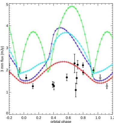
The resulting 3 mm fluxes are shown in Fig.3 (dark blue curve). We note that the general flux level is too high, as is the flux range. One should take into consideration that no parame-ters were adjusted in the modelling, and some quantities are not well known (e.g., the fraction of the shock energy that is trans-ferred to the relativistic electrons). Because the predicted flux levels coincide within an order of magnitude with the observa-tions, the curve can be viewed as indicative of the physical pro-cesses in play but it clearly does not tell the whole story. Note that whenBlomme et al.(2010) applied this same model to the 6 cm observations of Cyg OB2 #8A, they obtained theoretical fluxes that are systematically too low. The maximum of the the-oretical light curve is approximately as broad as the observed one. The main discrepancy is that this theoretical maximum is phase shifted with respect to the observations.
Blomme et al. (2010) also presented a model with stellar wind parameters for the primary that are different from the De Becker et al. (2006) ones ( ˙M = 1.0×10⁻⁶ M
yr−1, 3∞ = 2500 km s−1). While this helped to explain some features of the 6 cm observations, using these values for the 3 mm observations
-0.2 0.0 0.2 0.4 0.6 0.8 1.0 1.2
orbital phase 0
1 2 3 4 5
3 mm flux (mJy)
Fig. 3. Theoretical fluxes compared to the observed 3 mm fluxes of Cyg OB2 #8A, plotted as a function of orbital phase in the 21.908-day binary period. The black symbols with error bars show the observed data. Open symbols indicate duplications in the extended phase range (as in Fig.2). The dark blue curve is the synchrotron model, the red curve the adiabatic thermal emission model, the green curve the radia-tive thermal emission model, and the light blue curve the combined syn-chrotron and adiabatic thermal emission model.
only shifts the maximum even further away from the observed one.
A possible explanation for the phase shift of the maximum is our neglect of the orbital motion on the shape of the CWR. On a large scale, the contact discontinuity and its associated shocks take on the shape of a spiral, as shown by Parkin & Pittard (2008) using a simplified dynamical model. This spiral shape is confirmed by the full hydrodynamical models of e.g., ηCar (Parkin et al. 2011;Madura et al. 2013). For the purposes of un-derstanding the effect on the 3 mm fluxes of Cyg OB2 #8A, however, one needs to focus on a smaller scale, which extends only somewhat beyond theRτ=1 distances of 220 and 140R. At this scale the orbital motion pushes the leading edge of the CWR closer to the star with the weaker wind (see, e.g., Fig. 13 ofParkin et al. 2011). The position of the leading CWR edge in a model that does include orbital motion is therefore approxi-mately the same as the position at an earlier phase in a model that does not include orbital motion. A first-order correction of our theoretical light curve is therefore a shift of the curve to-wards the right in the orbital phase diagram. This is indeed the correct direction to improve the agreement of the theoretical and observed phases of maximum. Of course, we cannot estimate the size of the shift from this qualitative argument. For this we would need detailed hydrodynamical calculations, which are outside the scope of this paper.
5.3. CWR thermal emission – adiabatic model
-600 -400 -200 0 200 400 600 -600
-400 -200 0 200 400 600
y (R
O
•
)
phase = 0.125
-600 -400 -200 0 200 400 600
-600 -400 -200 0 200 400 600
phase = 0.325
-600 -400 -200 0 200 400 600
x (RO •) -600
-400 -200 0 200 400 600
y (R
O
•
)
phase = 0.650
-600 -400 -200 0 200 400 600
x (RO •) -600
-400 -200 0 200 400 600
phase = 0.925
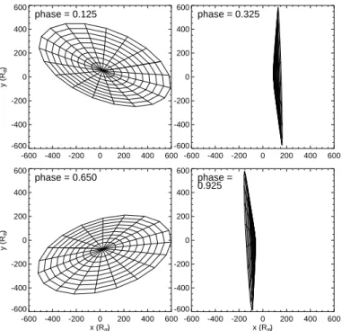
Fig. 4.CWR of the thin radiative shock model projected on to the sky, for phases where the flux is high (left column) and where the flux is low (right column). The orbital phase is listed in the top left corner of each panel. For plotting purposes, the CWR has been cut offat a distance of 600R.
free-free emission and absorption) to the observed fluxes. It is expected that the highly compressed material in the CWR will also contribute free-free emission and absorption, which could be detectable in the observations (Stevens 1995; Pittard 2010; Montes et al. 2011).
To explore the effect of the thermal emission, we use another radiative transfer model, developed byBlomme & Volpi(2014). This model uses an adaptive grid scheme allowing us to effi -ciently determine the emergent intensities and flux from the stel-lar winds and the CWR. The CWR is assumed to have a shape that is centred around a cone. The position and opening angle of this cone are determined analytically (Eichler & Usov 1993, their Eqs. (1) and (3)). The CWR has a half flaring angle (α), so it is thin at the apex and expands as we move away from the line connecting the two stars (see Fig. 2 of Blomme & Volpi). The size of the CWR scales with the distance between the two stars. We assume that the density inside the CWR is four times higher than what the wind density would be at that distance (this assumption will be revised in another model we discuss – see Sect.5.4). We refer to theBlomme & Volpipaper for further de-tails of the model.
For each phase of the orbit, we put the two stars in a three-dimensional grid, and assign the densities and temperatures of the stellar winds to each cell. The temperature of the CWR mate-rial is a free parameter; the wind matemate-rial is assumed to be at half of the effective temperatures of the stars. The grid is 16 000R on each side, and we start with 2563cells. We then solve the ra-diative transfer equation taking into account the free-free emis-sion and absorption, and refining the cells where needed (adap-tive grid scheme).
We explored a range of values for the temperature of the CWR, its flaring angle, and its size. The best fit we found (as judged by eye) is shown in Fig. 3 (red curve). Its parameters are a CWR temperature of 1.2×10⁵ K, a half-flaring angle of
30◦and a size of 1.8 times the separation between the two stars. These parameters were chosen from a large set of experiments, because they get the average flux level and the range of fluxes approximately correct. Similarly as for the synchrotron model, however, the maximum is phase shifted with respect to the ob-servations. It is also broader than observed. The use of the alter-nativeBlomme et al.(2010) model (with a lower mass-loss rate for the primary) does not solve the problem of the phase-shifted maximum. Similarly as in Sect.5.2, the phase shift can probably be attributed to our neglect of orbital motion.
To find out how much the CWR is contributing to the total flux, we also ran a model without a CWR, by setting the flar-ing angle to zero. We then find that the 3 mm flux varies be-tween 1.32 and 1.39 mJy, which is just marginally below the minimum of the red curve in Fig.3. The two stellar winds there-fore provide the “baseline” flux, and the CWR is responsible for the variability on top of that baseline flux. The CWR region is undetectable around phase 0.0–0.2 because the primary with the strongest wind is in front of it (conjunction is at phase 0.08). The free-free absorption in the stellar wind blocks most of the flux from the CWR. Around phase 0.4, the two stars are well separated on the sky, and that part of the CWR region which is beyond the free-free absorption of the stellar winds becomes detectable. At later phases, the secondary with the weaker wind moves in front (conjunction at phase 0.71), which reduces the detectable flux again, but not so much as when the primary was in front.
5.4. CWR thermal emission – radiative model
The model in the previous section limits the density contrast in the CWR to a factor of four. This is appropriate for an adia-batic shock. But, at least in part of the orbit the shock will be radiative, and the density contrast could be higher. This can be seen from the values of the cooling parameterχ, as defined by Stevens et al.(1992). De Becker et al.(2006) derived χ values for Cyg OB2 #8A which are around one (0.19–1.65, depend-ing on component and orbital phase; see their Table 11). This indicates that the shocks are radiative at least part of the time (near periastron, whereχ1), and can become adiabatic near apastron.
We therefore adapted the Blomme & Volpi (2014) code to include the semi-analytical model for radiative shocks in collid-ing stellar winds developed byMontes et al.(2011). This model assumes that the post-shock cooling is very efficient, leading to a thin CWR with a high density contrast, and a temperature that is equal to the wind temperature.Montes et al.determine the posi-tion of the contact discontinuity semi-analytically, and from the conservation equations they derive the surface density and emis-sion measure of the CWR material. To avoid substantial changes to our code, we do not directly use the emission measure, but we convert it into a density in a region around the contact disconti-nuity. As a standard value, we take 20Rfor the width of that region.
An important element in this explanation is that the CWR still has a significant flux contribution beyond the free-free ab-sorption region of the stellar winds. E.g., at phase 0.325, the sep-aration of the two stars on the sky is about 160R, which should be compared to theRτ=1 radii of 220Rand 140R(Table4). Although theseRτ=1 radii are based on an assumed spherically symmetric wind, they still indicate that the part of the CWR clos-est its apex will not be detectable. In contrast to this, for the adia-batic model from Sect.5.3(red curve on Fig.3) we have limited the size of the CWR to 1.8 times the separation between the two stars, so the CWR is only just beyond theRτ=1radius. Hence, it does not show the double wave effect. Of course, also in the adi-abatic model we could take a much larger limit on the size of the CWR, and in that case we would also get a double wave pattern. As this does not fit the observations, however, we did not present such models. Applying theBlomme et al.(2010) alternative stel-lar wind parameters (lower mass-loss rate for the primary) in the radiative model results in a similar double-wave pattern.
5.5. CWR combined synchrotron and adiabatic model
We can now extend the synchrotron model of Sect.5.2to also include the free-free emission and absorption of the CWR. In the Blomme et al.(2010) computer code, we find those cells where the synchrotron emission is non-zero, and we add the free-free opacity and emissivity, using a density four times higher than the local stellar wind density. We consider the temperature of the CWR wind to be a free parameter.
The resulting 3 mm fluxes are shown in Fig.3 (light blue curve). We used a CWR temperature of 7.0×10⁴ K, which is lower than the value used in Sect.5.3to avoid having fluxes that are too high. The combined model is comparable in quality of fit to the pure synchrotron one. The phase of maximum is shifted slightly toward the observed maximum, but is still quite some distance from it.
5.6. Comparison toPittard(2010)
Pittard(2010) used his 3D hydrodynamical models of colliding-wind binaries to predict thethermalemission from submillime-tre to centimesubmillime-tre radio wavelengths. Three of the four models he calculated have circular orbits, and are therefore not applicable to the eccentric binary Cyg OB2 #8A. This is further confirmed by the fact that all three predicted 3 mm light curves show a double peak, which is not seen in the Cyg OB2 #8A data.
ThePittard(2010) cwb4 model is an eccentric binary, though with parameters different from Cyg OB2 #8A: it is an O6V+ O6V system with a period of 6.1 days, and an eccentricity of e= 0.36. Each of the components has a mass loss rate of ˙M = 2×10⁻⁷ Myr−1. and a terminal velocity of3∞=2500 km s−1. Nevertheless, the hydrodynamics are somewhat similar to what we expect for Cyg OB2 #8A, in that the CWR is radiative at periastron and adiabatic at apastron. A qualitative comparison is therefore possible.
The cwb4 model shows a single peak in the 3 mm light curve, that is close to periastron. The exact orbital phase of the peak is only slightly dependent on the viewing angle. The observed data however, peak around phase 0.8. The difference could be due to the fact that the cwb4 model is for two equal winds, while the Cyg OB2 #8A winds are not equal. This will shift the phase of maximum away from periastron, but detailed hydrodynamical calculations of the Cyg OB2 #8A system would be required to see if the maximum moves to the observed one. The flux level of
the cwb4 peak is about three times the baseline flux. This com-pares well to the factor of about two seen in the Cyg OB2 #8A data.
6. Cyg OB2 #8B
On the map of our combined data (Fig. 1) we also detected Cyg OB2 #8B (=Schulte 8B=MT 462). We measured its flux on the combined visibility data, by fitting a model with two point sources (one for #8A, and one for #8B). We found a flux for Cyg OB2 #8B of 0.21±0.033 mJy, with a position that is offset by only 000.4 from its SIMBAD position.
In order to convert the observed flux into a mass-loss rate, we need to know additional information about this star. Its spectral type is listed as O6 II(f) (Sota et al. 2011), O6.5 III(f) (Massey & Thompson 1991), or O7 III-II (Kiminki et al. 2007). There are no significant radial velocity changes (Kobulnicky et al. 2014), making it unlikely that it is a binary.
There are no stellar parameter determinations for this star, so we have to rely on calibrations to determine them. We fol-lowMorford et al.(2016), who use theMartins et al.(2005) cal-ibration to derive an effective temperature Teff = 35 644 K, a luminosity of logL/L = 5.49, and a (spectroscopic) mass of M/M=33.68, based on the O6.5 III(f) spectral type. From the Prinja et al.(1990) calibration of terminal velocity versus spec-tral type,3∞ = 2545 km s−1 follows. Using this in Eq. (1), we find ˙M=1.42±0.2×10⁻⁶ Myr−1.
We can compare this to the upper limits that have been de-rived from radio observations.Morford et al. (2016) derive an upper limit from their 21 cm observations of 0.078 mJy, cor-responding to ˙M < 4.3 ×10⁻⁶ Myr−1. The 0.2 mJy upper limit at 6 cm found by Bieging et al. (1989) leads to ˙M < 5.2×10⁻⁶Myr−1. There are no determinations from other mass loss indicators (such as Hα). It should be noted that all mass-loss rates listed here have not been clumping corrected.
The predicted mass-loss rate according to the Vink et al. (2001) formulae is 0.7×10⁻⁶ Myr−1. The difference between this value and the observed one can be interpreted as due to clumping, with a clumping factor of four. This value is com-patible with current ideas about clumping in massive-star winds (e.g.,Puls et al. 2008).
7. Conclusions
We monitored the massive colliding-wind binary Cyg OB2 #8A at 3 mm with the NOEMA interferometer, with good phase cov-erage of its orbit. For 12 of the 14 observations, we could deter-mine the flux.
The 3 mm light curve shows clear phase-locked variabil-ity, indicating that a substantial part of the flux comes from the colliding-wind region (CWR)3. We modelled the data us-ing models that include synchrotron radiation due to the CWR, or free-free emission from the CWR, or both. All models give fluxes and flux ranges higher than those observed, though com-parable in magnitude to the observations. With the exception of
3 One could consider alternative explanations, such as phase-locked
the radiative shock model, all have a single peak – as observed. The slightly better agreement of the shape of the maximum would favour the synchrotron interpretation. From a modelling point of view, however, some contribution of free-free emission from the CWR is also expected. In summary, stronger arguments will be required for a decision on how much each of the two emission mechanisms contribute to the observed fluxes.
The main problem with the models presented here is that the theoretical maxima are phase shifted with respect to the observed one. It is clear that, at least qualitatively, this is due to our ne-glect of the orbital motion on the shape of the CWR. To see if this is also quantitatively the correct explanation, more sophisti-cated modelling will be required. This should be based on solv-ing the hydrodynamical equations, in order to derive the density and temperature distribution in the CWR. These can then be used to calculate a better theoretical light curve and will allow us to determine the relative contributions of the synchrotron and free-free radiation emission.
On the deep 3 mm image made by combining all our data, we also detected the visual companion Cyg OB2 #8B. We measured a flux of 0.21±0.033 mJy, which leads to a (non-clumped) mass-loss rate of ˙M=1.42±0.2×10⁻⁶Myr−1. From a comparison with predicted mass-loss rates, we derive a clumping factor of four, which is compatible with current ideas about clumping in massive-star winds.
Acknowledgements. We are especially grateful to Jan Martin Winters and Charlène Lefèvre (IRAM) for their assistance with the data reduction. We thank the referee for his/her comments, which helped to improve the paper. We have made use of the GILDAS software for the reduction of the data. This research has made use of the SIMBAD database, operated at CDS, Strasbourg, France and NASA’s Astrophysics Data System Abstract Service. J. Morford and D. Fenech wish to acknowledge funding from an STFC studentship and STFC consolidated grant (ST/M001334/1) respectively.
References
Bell, A. R. 1978,MNRAS, 182, 147
Benaglia, P., & Romero, G. E. 2003,A&A, 399, 1121
Benaglia, P., Marcote, B., Moldón, J., et al. 2015,A&A, 579, A99
Bieging, J. H., Abbott, D. C., & Churchwell, E. B. 1989,ApJ, 340, 518
Blomme, R., & Volpi, D. 2014,A&A, 561, A18
Blomme, R., Van Loo, S., De Becker, M., et al. 2005,A&A, 436, 1033
Blomme, R., De Becker, M., Runacres, M. C., Van Loo, S., & Setia Gunawan, D. Y. A. 2007,A&A, 464, 701
Blomme, R., De Becker, M., Volpi, D., & Rauw, G. 2010,A&A, 519, A111
Blomme, R., Nazé, Y., Volpi, D., et al. 2013,A&A, 550, A90
Daley-Yates, S., Stevens, I. R., & Crossland, T. D. 2016,MNRAS, 463, 2735
De Becker, M. 2007,A&ARv, 14, 171
De Becker, M., Rauw, G., & Manfroid, J. 2004,A&A, 424, L39
De Becker, M., Rauw, G., Sana, H., et al. 2006,MNRAS, 371, 1280
Dougherty, S. M., Pittard, J. M., Kasian, L., et al. 2003,A&A, 409, 217
Eichler, D., & Usov, V. 1993,ApJ, 402, 271
Ginzburg, V. L., & Syrovatskii, S. I. 1965,ARA&A, 3, 297
Kennedy, M., Dougherty, S. M., Fink, A., & Williams, P. M. 2010,ApJ, 709, 632
Kiminki, D. C., Kobulnicky, H. A., Kinemuchi, K., et al. 2007,ApJ, 664, 1102
Knödlseder, J. 2000,A&A, 360, 539
Kobulnicky, H. A., Kiminki, D. C., Lundquist, M. J., et al. 2014,ApJS, 213, 34
Leitherer, C., & Robert, C. 1991,ApJ, 377, 629
Madura, T. I., Gull, T. R., Okazaki, A. T., et al. 2013,MNRAS, 436, 3820
Martins, F., Schaerer, D., & Hillier, D. J. 2005,A&A, 436, 1049
Massey, P., & Thompson, A. B. 1991,AJ, 101, 1408
Montes, G., González, R. F., Cantó, J., Pérez-Torres, M. A., & Alberdi, A. 2011,
A&A, 531, A52
Montes, G., Alberdi, A., Pérez-Torres, M. A., & González, R. F. 2015,Rev. Mex. Astron. Astrofis., 51, 209
Morford, J. C., Fenech, D. M., Prinja, R. K., Blomme, R., & Yates, J. A. 2016,
MNRAS, 463, 763
Parkin, E. R., & Pittard, J. M. 2008,MNRAS, 388, 1047
Parkin, E. R., Pittard, J. M., Corcoran, M. F., & Hamaguchi, K. 2011,ApJ, 726, 105
Pittard, J. M. 2007,ApJ, 660, L141
Pittard, J. M. 2010,MNRAS, 403, 1633
Pittard, J. M., & Dougherty, S. M. 2006,MNRAS, 372, 801
Pittard, J. M., Dougherty, S. M., Coker, R. F., O’Connor, E., & Bolingbroke, N. J. 2006,A&A, 446, 1001
Pollock, A. M. T. 1987,A&A, 171, 135
Prilutskii, O. F., & Usov, V. V. 1976,Sov. Astron., 20, 2
Prinja, R. K., Barlow, M. J., & Howarth, I. D. 1990,ApJ, 361, 607
Puls, J., Vink, J. S., & Najarro, F. 2008,A&ARv, 16, 209
Rauw, G., & Nazé, Y. 2016,Adv. Space Res., 58, 761
Reimer, A., Pohl, M., & Reimer, O. 2006,ApJ, 644, 1118
Reitberger, K., Kissmann, R., Reimer, A., & Reimer, O. 2014,ApJ, 789, 87
Sota, A., Maíz Apellániz, J., Walborn, N. R., et al. 2011,ApJS, 193, 24
Stevens, I. R. 1995,MNRAS, 277, 163
Stevens, I. R., & Pollock, A. M. T. 1994,MNRAS, 269, 226
Stevens, I. R., Blondin, J. M., & Pollock, A. M. T. 1992,ApJ, 386, 265
Van Loo, S., Runacres, M. C., & Blomme, R. 2005,A&A, 433, 313
Van Loo, S., Blomme, R., Dougherty, S. M., & Runacres, M. C. 2008,A&A, 483, 585
Vink, J. S., de Koter, A., & Lamers, H. J. G. L. M. 2001,A&A, 369, 574
White, R. L., & Becker, R. H. 1995,ApJ, 451, 352
Wright, A. E., & Barlow, M. J. 1975,MNRAS, 170, 41