Errors of Measurement: Regression Toward the Mean

Version: Accepted Version

Book Section:

Bland, John Martin orcid.org/0000-0002-9525-5334 (2017) Errors of Measurement: Regression Toward the Mean. In: Allen, Mike, (ed.) The SAGE Encyclopedia of

Communication Research Methods. SAGE Publications , Thousand Oaks , pp. 441-446.

Reuse

The SAGE Encyclopedia of

Communication Research Methods

Errors of Measurement: Regression Toward the

Mean

Contributors: Martin Bland Edited by: Mike Allen

Book Title: The SAGE Encyclopedia of Communication Research Methods Chapter Title: "Errors of Measurement: Regression Toward the Mean" Pub. Date: 2017

Access Date: May 18, 2017

Publishing Company: SAGE Publications, Inc City: Thousand Oaks

Print ISBN: 9781483381435 Online ISBN: 9781483381411

DOI: http://dx.doi.org/10.4135/9781483381411.n164 Print pages: 441-446

©2017 SAGE Publications, Inc. All Rights Reserved.

In 1886, Francis Galton published an article titled “Regression Towards Mediocrity in Hereditary Stature.” Interested in heredity, Galton had obtained measurements on heights of 205 sets of parents and their 913 adult children. He noticed that if he selected families where the parents were tall, the average height of the children was less than that of their parents, whereas if he selected families where the parents were short, the average height of the children was greater. Galton called this “regression towards mediocrity”; it is now known as “regression towards the mean,” as the term mediocrity has acquired disparaging connotations.

The same thing happens with the children: for tall children, the mean height of their parents is less; for short children, the mean height of their parents is greater. This is a statistical, not a genetic, phenomenon. This entry discusses how regression toward the mean works, providing several examples.

How Regression Toward the Mean Works

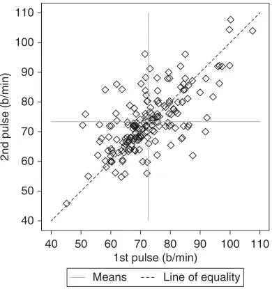
Galton’s data were quite complicated, with adjustment for gender and multiple children per family. In this entry, a much simpler data set is presented to see how regression works: pulse rate for 185 students, each student measured by two other students. The data are shown in Figure 1. This figure also shows lines through the means of the first and second measurement and the line of equality, on which the points would lie if the two measurements were identical. The horizontal and vertical lines cross very close to the line of equality, because the means of the first and second measurements are almost the same, 72.6 and 73.3 beats per minute (b/min), respectively. The spread of the distributions is almost the same, too. The minima are 45 and 46 b/min, the maxima are both 108 b/min, and the standard deviations are 10.4 and 9.8 b/min.

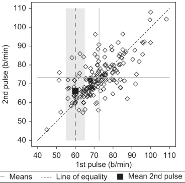
Because the two pulse measurements were conducted during the same practical class, they should be the same, except for measurement error. What is the mean second pulse measurement for students whose first pulse is 60 b/min? Will it be 60 b/min? Not many first measurements are exactly 60, so all measurements between 55 and 65 b/min are considered. As Figure 2 shows, the mean second pulse is greater than 60 b/min; it is 66.2 b/min, closer to the mean than is 60 b/min.

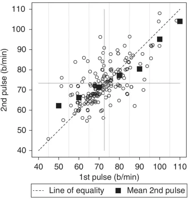
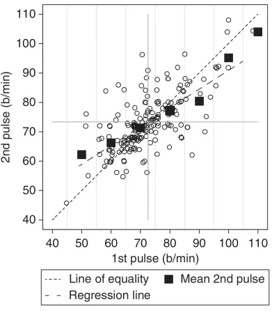
This can also be done for the first pulse, as shown in Figure 3. These means do not lie on the line of equality but on one which crosses it, as shown in Figure 4.

The means in Figure 3 lie on the simple linear regression line, approximately. When statisticians estimate the line that best fits the data in a scatterplot diagram like Figure 1, they find the line that best predicts the mean value of one of the variables, called the outcome, dependent, or y variable, from the observed value of the other, called the predictor, explanatory, independent, or x variable. The line chosen is the one that makes a minimum of the differences between the observed values of the y variable and the mean values that would be predicted by the line. It minimizes the sum of the squares differences between the observed and predicted values. The method has its roots in Galton’s article, hence the name regression line. The line shown in Figure 4 is called the regression of second pulse on first pulse.

Figure 2 Pulse Data Showing the Mean Second Pulse for Those Whose First Pulse is Between 55 and 65 b/min

SAGE SAGE Reference

Figure 4 Mean of Second Pulse for Students Grouped by First Pulse in Groups of Width 10 b/min, With Linear Regression Line

SAGE SAGE Reference

Regression toward the mean works in the same way even if one were to start with the second measurement and find the mean of the first. For example, the average first pulse measurement for students whose second measurement was between 55 and 65 b/min was 65 b/min. Again, it is closer to the mean than is the pulse by which observations were selected. Figure 5 shows the first pulse for students grouped by second pulse. The mean first pulse for a given value of the second pulse lies on a different regression line from the second grouped by the first. This is the regression of first pulse on second pulse, minimizing the sum of the squared differences between the first pulse and the value predicted by the line.

Figure 6 The Two Regression Lines

SAGE SAGE Reference

There are two regression lines, as shown in Figure 6. Neither is the same as the line of equality. This represents the true, functional relationship between the pulses, without any measurement error, which is that they are the same. All three lines, both regressions and equality, go through the mean point.

Regression toward the mean can happen in several different types of study. The study of heredity is just one. The following section provides several examples.

regression toward the mean.

Another example involves a study of reoffending by ex-prisoners. A UK government minister was reported as claiming that prison sentences work, because following release from prison, the next offense for which ex-prisoners were convicted tended to be for a less serious crime than the one that had led to the prison sentence. But this would be expected. Because more serious crimes are more likely to be punished by prison sentences, ex-prisoners are a group selected because their last crime was at the serious end of the distribution. Hence, the “average seriousness” of their next crime will be lower, simply due to regression toward the mean.

It is often suggested that street lighting should be improved to reduce crime or traffic accidents. It is argued that when an area of high crime is given improved street lighting or where an accident black spot has some traffic-calming measure introduced, and crime or accidents fall, the change has produced the effect. But if this change was made only because the area was selected as having a high rate of crime or accidents, high rate areas are likely to decrease as a result of regression toward the mean. Even if one were to compare an area where street lighting has been improved with an area where it has not, as a control group, the intervention is not allocated at random. It is usually carried out in the area with the higher crime rate, so regression toward the mean may still influence the result. Paul Marchant compared the change in burglary rates in 124 areas where there were data for successive years. He reported that in the areas with a baseline rate above the mean, the mean fall in the number of burglaries was 71, but in the low-rate group, there was a mean increase of 5.9 burglaries.

The UK government once reported that underperforming primary schools were raising their standards significantly. This was based on league tables for results in tests taken by 11-year-olds in England. Improvements were best in schools where fewer than two thirds of pupils previously achieved at least Level 4, the standard expected of children in the age group. But one would expect the worst performing schools to improve and the best to decline, simply as a result of regression toward the mean.

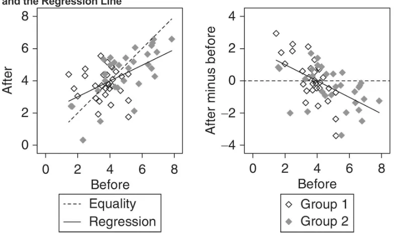
Figure 7 Simulation of Measurements Before and After Intervention, Showing the Line of Equality and the Regression Line

SAGE SAGE Reference

Comparing Differences From Baseline

In a comparative trial, researchers may measure their outcome variable both before and after treatment. Because the baseline and outcome measurements are almost certain to be correlated, using the baseline information in the analysis should improve the precision of the treatment estimate. Sometimes, researchers might also observe some imbalance between groups on baseline, despite randomization. They might be tempted to take posttreatment measurement minus baseline measurement as the outcome variable for their analysis.

As Figure 7 illustrates, any imbalance will be reversed, due to regression toward the mean. In this simulation, the correlation between the before and after measurements is r = .5. Figure 7 shows that observations that have a high before measurement tend to have a high after measurement, as one might expect, but also tend to have a lower measurement after than before. In the same way, observations that have a low before measurement tend to have a higher measurement after than before. This means that the difference, after minus before, tends to be positive when the baseline is low and negative when baseline is high. Thus, if there is an imbalance, as in the simulation, where Group 2 has slightly higher baseline measurements than Group 1, the differences are lower in the higher baseline group. Group 2 has more negative differences than Group 1.

Using the difference between posttreatment and baseline measurements is ill-advised not only because of regression toward the mean but also because of increased measurement error. When one subtracts one measurement from another, some of the variability due to the person may be removed; the variability due to the measurement process itself is doubled, because it is from the baseline and the posttreatment measurements. Instead, researchers should compare the groups for the posttreatment measurement, adjusting for the baseline using a method called analysis of covariance or multiple regression, which solves both the problem of increased error and that of regression toward the mean.

If researchers select participants for a study based on a measurement being in a specified range, then the same measurement as the baseline should not be used in the analysis. It is better to make a duplicate baseline measurement. The researchers then use one baseline to select subjects and use the other in the analysis. The reason for this is that a group selected as being above a cutoff, for example, will have a lower mean value when measured again. The cutoff measurement will be a biased estimate of the true value of the quantity being measured.

Relating Change to Initial Value

Researchers may be interested in the relation between the initial value of a measurement and the change in that quantity over time. In anti-hypertensive drug trials, for example, it may be postulated that the drug’s effectiveness would be different (usually greater) for patients with more severe hypertension. Regression toward the mean will be greater for the patients with the highest initial blood pressures, so that one would expect to observe the postulated effect even in untreated patients.

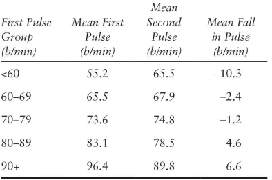
Table 1 shows this for the pulse rate data, where no systematic change has taken place at all, even due to time. Those with the highest first pulse have the greatest fall in pulse from first measurement to second; those with the lowest first pulse have the highest increase to the second. Because of these regression toward the mean effects, the estimation of any additional effect of treatment is very difficult and a specialized job.

Table 1 Mean Fall in Pulse Rate From the First to the Second Measurement, Grouped by First Pulse Measurement

Agreement Between Two Methods of Measurement

SAGE SAGE Reference

For example, several researchers have compared self-reported weight of survey respondents to their weight as recorded using scales. They then carry out regression of reported weight on measured weight and find that the slope is less than 1.0. They conclude that underweight people tend to overestimate their weight and overweight people tend to underestimate their weight. But the slope less than 1.0 is exactly what would be expected if the two weights are exactly the same apart from measurement error, just as in Figure 4. Under those circumstances, they would also get a slope less than 1.0 if they did regression of measured weight on reported weight.

Regression Toward the Mean Is Everywhere

Once one becomes aware of regression toward the mean, one may begin to see it everywhere. Consider, for example, a study from education. In this study, children were defined to be “gifted” if their intelligence quotient exceeded a particular cutoff. School attainment was measured with other scales. The researcher found that mean attainment score was fewer standard deviations above the population mean than was the mean intelligence quotient for this group. This was interpreted as showing that schools were failing “gifted” children. But it is exactly what regression toward the mean would lead one to expect.

Two famous examples of regression toward the mean are the “Curse of Hello” and the “Sports Illustrated jinx.” People who appear on the covers of these magazines often have bad things happen to them afterward: their movie flops or their team loses, for example. But one only gets on these covers if one has recently been unusually successful. Regression toward the mean predicts that, on average, cover stars will be less successful after appearing on the cover.

As shown in this entry, regression toward the mean is a frequently occurring phenomenon. It can be estimated in some cases or it can be avoided by design. It can make many traps for the unwary, so it is important to be aware.

Martin Bland

See alsoCross-Lagged Panel Analysis; Delayed Measurement; Errors of Measurement; Experiments and Experimental Design; Reaction Time; Reliability of Measurement; Repeated Measures; t-Test, Paired Samples; Within-Subjects Design

Further Readings

Andersen, B. (1990). Methodological errors in medical research: An incomplete catalogue. Oxford, UK: Blackwell.

Chinn, S., & Heller, R. F. (1981). Some further results concerning regression to the mean. American Journal of Epidemiology, 114, 902–905.

Davis, C. E. (1976). The effect of regression to the mean in epidemiologic and clinical studies. American Journal of Epidemiology, 104, 493–498.

Galton, F. (1886). Regression towards mediocrity in hereditary stature. Journal of the Anthropological Institute, 15, 246–263.

Hayes, R. J. (1988). Methods for assessing whether change depends on initial value. Statistics in Medicine, 7, 915–927.

James, K. E. (1973). Regression toward the mean in uncontrolled clinical studies. Biometrics, 29, 121–130.

Marchant, P. (2005). Evaluating area-wide crime-reduction measures. Significance, 3, 62–65. Mee, R. W., & Tin, C. C. (1991). Regression towards the mean and the paired sample t test. American Statistician, 45, 39–42.

Reader, R., Bauer, G. E., & Doyle, A. E. (1980). The Australian trial in mild hypertension: Report by the management committee. Lancet, 1, 1261–1267.

Senn, S. J., & Brown, R. A. (1985) Estimating treatment effects in clinical trials subject to regression to the mean. Biometrics, 41, 555–560.

Shepard, D. S., & Finison, L. J. (1983). Blood pressure reductions: Correcting for regression towards the mean. Preventive Medicine, 12, 304–317.

Martin Bland

http://dx.doi.org/10.4135/9781483381411.n164 10.4135/9781483381411.n164

SAGE SAGE Reference