Neural networks and the interpolation of sparse earth-science data

(1)

Neural Networks and the Interpolation of

Sparse Earth-Science Data

Ernest Yiu Cheong Wan

February, 1998

(2)

Part of the work presented in the thesis has been published in the papers:

Wan, E. & Bone, D. (1996). A neural network approach to covariation model fitting and the

interpolation of sparse earth-science data. In Proceedings o f the Seventh Australian Conference on Neural Networks, pp. 121-126; and

Wan, E. & Bone, D. (1997). Interpolating earth-science data using RBF networks and mixtures

of experts. In Advances in Neural Information Processing Systems 9, (eds.) M. C. Mozer, M. I. Jordan, T. Petsche, MIT press, Cambridge, Mass, pp. 988-994.

Except where otherwise acknowledged, the work presented in this thesis is solely that of

the author.

Statement of Originality

(3)

Acknowledgments

I would like to thank my advisors Dr. Robert Williamson, Dr. Donald Bone and Dr. Anthony Burkitt for their support, criticism and advice. I am especially grateful to Don for having to put up with me on a daily basis and for his stimulating thoughts and continuing encouragement. Also, the thesis would have never arrived had it not been Bob’s effort in keeping me realistic on the scope of the thesis and helping me to plan my study. A special thanks to Prof. Donald Fraser and Dr. Thomas Graham Freeman who encouraged me to take up the PhD studies in the first place.

I am grateful to CSIRO for providing me with an office and their computing facilities, and to Kevin Smith for overseeing the funding for this research. I wish also to thank my fellow PhD students and the researchers especially Andrew Lui and Dr. Hong Xin He, at the Canberra Laboratory of CSIRO for their friendship and ideas.

(4)

Abstract

A neural network approach is developed for the interpolation of sparse, spatially correlated earth-science data. It is shown that (universal) kriging , an interpolation method widely used in geostatistics, is formally equivalent to generalized radial basis function networks (GRBFN) that have an RBF units at each data points. The formal relationship provides a strong foundation and justification for a GRBFN approach to the problem.

The kriging approach uses a covariation model which specifies the spatial variability in the data to derive the optimal unbiased linear predictor for unsampled locations.

However, the covariation model is in general unknown and has to be estimated from the data. Estimating the model from earth-science data has proved to be difficult in practice due to the sparseness of the data samples. Furthermore for many data sets, the samples are not collected from a single homogeneous area and, hence, cannot be accurately described by a global covariation model.

Based on the formal relationship between kriging and GRBFN, an empirical Bayesian approach is developed to train a GRBFN to learn the covariation model and interpolate the data. Simulation results show that the neural network approach outperforms traditional geostatistical methods in estimating the covariation model resulting in improved prediction accuracy.

Based on the idea of hierarchical mixtures of experts (HME), the approach is extended to use a hierarchy of GRBFNs to soft partition the input space into regions with similar covariation behavior, learn the local covariation models and combine the predictions of the local GRBFN experts. Instead of computing the ML estimates, the original

expectation-maximization (EM) training algorithm of HME is extended to include priors on the parameters of the experts to improve generalization. Results on simulated and real non-homogeneous data sets show significant improvement in prediction

(5)

The partitioning and model fitting problems currently represent the most time

consuming part of the kriging process, in part because they involve a large amount of manual intervention. The current work provides an automated solution to these

problems while conforms with the kriging model. In addition, the new approach allows the two problems to be resolved in the same neural network framework allowing

(6)

List of Figures

Figure 1.1 The typical steps of the kriging process... 3

Figure 1.2 A typical backpropagation netw o rk ...13

Figure 1.3 A standard radial basis function netw ork... 14

Figure 2.1 A typical semivariogram... 27

Figure 2.2 A rose diagram of the range of nine directional sample variograms whose directions lie on a 2D p lan e...30

Figure 2.3 The three angles which define the orientation of the anisotropy...32

Figure 4.1 The equivalent network implementation of an ordinary cokriging system with 2 output variables - a primary and a secondary... 100

Figure 5.1 The ID function y = sin(10x) and the 50-points noisy training set...105

Figure 5.2 The semivariograms of the ID data set and the semivariogram models fitted to them by WLS and by e y e ...107

Figure 5.3 The log evidence and the maximum log posterior for the 11-Gaussian units GRBFN as a function of the scaling parameter a...109

Figure 5.4 The ID interpolant generated by a 50-Gaussian units GRBFN and by local ordinary kriging using the covariation model determined by the evidence procedure of algorithm 4 .2 ...110

Figure 5.5 The ID interpolant generated by a 50-Cauchy units using the covariation model determined by the evidence procedure of algorithm 4.2...111

Figure 5.6 (a) The 50x50 image and (b) the histogram of the simulated lognormal data set. The data set has an isotropic exponential circular variogram... 117

Figure 5.7 (a) The sample semivariograms and (b) the inverted sample correlograms of the exhaustive (top) and the ten lognormal sample data se ts...118

Figure 5.8 The exponential circular models fitted by WLS to (a) the sample semivariograms and (b) the inverted sample correlograms of the ten sample data sets of the lognormal d ata...121

Figure 5.9 (a) The interpolant generated by the GRBFN trained using the evidence procedure of algorithm 4.1 on sample 1, and the contours of the size of its 1 a error bars computed using (b) kriging variance and (c) the Bayesian prediction variance...122

Figure 5.10 The sample semivariograms of the ten sample data sets and the exponential semivariogram models fitted by W LS... 128

Figure 6.1 A typical balanced 2-level HME. Each expert can be further expanded into a gating network and a set of sub-experts to form a deeper tre e ... 135

Figure 7.1 The 2-level HME used for the experiments... 159

Figure 7.2 The profile of the true local covariation models of the simulated data s e t. 162 Figure 7.3 The profile of the local covariation models of the simulated data learned by the HME trained using algorithm 6 .2 ... 162

Figure 7.4 (a) The simulated data set and (b) the true partitions. The interpolants generated by (c) the HME and (d) the 64-unit GRBFN both trained using algorithm 6.2... 163

(10)

Figure 7.6 The profile of the local covariation models of the aero-magnetic data

learned by the HME trained using algorithm 6.2... 166 Figure 7.7 The outputs of the gating networks over the input space of the

aero-magnetic data set... 166 Figure 7.8 (a) The entire aero-magnetic data set. (b) The training set which consists

mainly of the inner flights paths, (c) Thin-plate interpolant of the entire aero- magnetic data set which was generated to help the readers to visualize the major features of the data, (d) The HME interpolant of the training set... 167

L ist of T a b le s

Table 5.1 The performance of the ordinary kriging predictor on the ID test set using the various models fitted to the sample semivariograms by WLS and by eye. The result of local ordinary kriging using the covariation model fitted by the evidence procedure is also shown... 108 Table 5.2 The models fitted by the GRBFNs and the performance of the GRBFNs

on the ID test set. Orr’s results using global ridge regression, local ridge

regression and forward selection are also shown for comparison...112 Table 5.3 The parameters of the exponential circular variogram models fitted to the

ten sample data sets by WLS, ML and the evidence procedure...119 Table 5.4 The normalized mean squared error (NMSE) on the unused data when the

estimated variogram models of table 5.3 and the true model are used for kriging. 120 Table 5.5 The parameters of the exponential semivariogram models fitted to the ten

sample data sets by WLS, MLCV, ML and the evidence procedure...127 Table 7.1 Normalized mean squared prediction error for the simulated data set... 160 Table 7.2 The parameters of the true local variogram models of the simulated data

set and those of the local variogram models learned by the HME trained using algorithm 6.1 and 6.2...161 Table 7.3 Normalized mean squared prediction error for the aero-magnetic data set.

All networks are trained using algorithm 6 .2 ... 165 Table 7.4 The parameters of the local variogram models learned by the HME trained

(11)

1. Introduction

In many earth science problems, one has a collection of measurements of a variable plus the geographic locations of the measurement points. One typically wants to interpolate between data points and extrapolate (a small distance) beyond the data. Interpolation of the available samples allows the study of shape and orientation of geographical features, inference of the presence of global trends, or estimation of local characteristics that are of interest.

The first problem with spatial data is the spatial dependence of the observations. Standard statistical techniques usually assume that observations of a phenomenon form a random sample, i.e. the observations are independently and identically distributed (or i.i.d.). For spatial data, observations that are close together in space are usually

positively correlated. The dependence becomes stronger as the distance between them decreases. Departures from independence need to be modeled.

The second problem with spatial data is that the spatial locations of data are often not regularly spaced and the spatial location is allowed to vary continuously over space. While time series models are usually based on identically distributed observations that are dependent and occur at equally spaced time points, spatial models have to be more general to allow for irregularly spaced data.

(12)

are typically sparse. One must take ones observations where one can and observations are too valuable to lightly discard.

The final problem is that very few earth science applications are sufficiently understood to permit a deterministic approach to prediction. Physicists can develop a somewhat idealized deterministic model to predict the path of a projectile because they know the controlling physical laws and forces. Earth scientists can seldom produce a

deterministic description of the process generating the data.

This thesis is concerned with developing artificial neural network (ANN) techniques to solve the problem of interpolating sparse, spatially correlated earth-science data.

Geostatistical methods are currently being used to deal with the interpolation problem. In this chapter, we will present some background information on geostatistics and

artificial neural networks (ANN). We will briefly describe kriging, the most widely used geostatistical solution, to the interpolation problem. We will discuss the major advantages and problems of the method. We will link kriging to other related interpolation methods including the radial basis functions (RBF) method of

interpolation, splines and RBF networks (RBFN), and point out their differences. In the case of ANN, we will briefly discuss its basic concepts and its main applications. In addition, we will describe the architecture of two popular classes of networks - RBFN and backpropagation networks (BPN). After introducing the two main fields of our research, we will then spell out the goals of the thesis stating the problems of kriging that we try to solve and the close connection between kriging and RBFN that motivates our approach. We will briefly describe other related works and the problems with the BPN approach they adopted. Finally, we will outline the structure of the rest of the thesis.

1.1 Geostatistics

Geostatistics is a special branch of applied statistics formalized by G. Matheron [Math62, Math63a, Math63b] at the Center de Morphologie Mathematique in

(13)

problems that arise when conventional statistical theory is used to infer ore reserves

within a mine. Its strength over classical approaches to ore-reserve estimation is that it

recognizes spatial variability at both the large scale and the small scale. That is, it

models both the spatial trend and spatial correlation, and makes use of the spatial

information in the data sets when making inferences. As spatial continuity is an

essential feature of many natural phenomena, geostatistics is also applicable in various

areas of geology and other earth sciences such as soil science, crop science, ecology,

forestry, astronomy, atmospheric science, etc. It has even been used in fields such as

image processing and epidemiology.

Most applications of geostatistics are related to mapping the spatial distribution of (or

interpolating) one or more attributes using an interpolation (or prediction) method

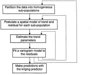
known as kriging, with emphasis given to characterizing the spatial dependence of the data with a variogram model and measuring the prediction accuracy using the kriging (error) variance. Figure 1.1 summarizes the typical steps of the kriging process which we will briefly describe in the following sections.

Estimate the trend parameters

Fit a variogram model to the residuals

Make predictions with the kriging predictor

Partition the data into homogeneous sub-populations

Postulate a spatial model of trend and residual for each sub-population

Figure 1.1 The typical steps of the kriging process. Note the trial-and-error approach in the partitioning of the data set and the fitting of an appropriate spatial model. The dotted arrows are possible backward paths that allow the partitioning and the spatial model to be adjusted if

[image:13.531.141.450.398.649.2]

(14)

1.1.1 Probabilistic Approach to Spatial Data Modeling

Interpolation from sparse sampling is an ill-posed problem. There are infinitely many possible interpolation surfaces from which to choose. When one has little knowledge of the process generating the surface, as in the case of many earth science applications, a standard approach is to deal with it statistically. In geostatistics, the process generating the surface is modeled as a random process. The observations are viewed as a partial realization of a random process.

Large-scale variation in the physical process is allowed for through the mean function of the random process which is usually referred to as the trend. The trend will have the form of a smooth approximation of the random process. If the trend is removed from the random process, the residual (or error process) will be a zero-mean random process. In addition, the residual will be stationary. Hence its spatial continuity can be measured by, say, a sample variogram or a set of directional sample variograms and characterized by a variogram model. Other second-order continuity measures such as the

covariogram and the correlogram can also be used instead of the variogram1. The variogram and variogram model are explained below in section 2.2.1 and 2.2.2

respectively. For details of the covariogram and the correlogram, see the book by Isaaks and Srivastava [Isa89]. We will refer to the various forms of spatial continuity model as

covariation models.

The two components of the spatial model - a deterministic trend and a stochastic residual - reflect a common belief among geologists that the surface is the outcome of two interacting sets of geological forces with one set shaping the region and the other causing small areas to deviate from the regional pattern.

(15)

also influences ones definition of the two spatial components. They depend very much on the particular application and the practitioner’s intuition, preferences, and his/her familiarity with the type of data. One persons deterministic trend may be the variogram structure of another persons stochastic residual.

The process of simultaneously finding satisfactory representations of the trend and the variogram structure of the residual is a principal concern of what is known as structural analysis in geostatistics. It is to some extent an art requiring experience and

experimentation as well as luck. Nevertheless, the kriging predictor used in

geostatistics is in general not very sensitive to the use of different spatial models i.e. different decompositions of trend and residual, provided that the model parameters are sensibly estimated. This is because any misspecification in the trend tends to be

compensated for in the variogram structure of the residual and vice versa. For example, if the trend is underfitted, the residual is automatically overfitted [Cre93].

In this thesis, we will not concern ourselves with the problem of non-unique

decomposition of the spatial model. We will concentrate on developing methods to ‘sensibly’ estimate the model parameters. More specifically, we will develop neural network techniques that result in better estimates of the model parameter and improved prediction accuracy.

1.1.2 Kriging

Kriging is a geostatistical interpolation method widely used in the earth sciences. It employs a linear predictor and is a minimum-mean-squared-error method of spatial prediction that depends on the second-order properties of the random process. Kriging requires a priori knowledge about the spatial variability of the data. In general, this is not known and is determined and modeled through an initial structural analysis on the data. The analysis finds a low order polynomial to characterize the trend and fits a

(16)

variogram model to the sample variogram(s) to characterize the spatial variability of the residuals.

Kriging evaluates the value at an unsampled location as a weighted sum of the sparse, spatially correlated sample points. Kriging uses the spatial information captured in the variogram model to find an optimal set of weights. The weights are optimal in the sense that the error variance is minimized. Under the unbiasedness constraint, minimizing the error variance is equivalent to minimizing the (expected) squared prediction error. Unlike other simple interpolation methods such as inverse distance methods and triangulation which only weight data points according to their distance from the unknown point, the kriging weights take account of the spatial correlation between the available data points and between the unknown points and the available data points. In doing so, kriging not only attributes more weight to observations closer to the unknown point, it also declusters the available observations. That is, observations that are

statistically close to each other are weighted less than if they are not. Another advantage kriging has over other interpolation methods is that it provides a measure of the error of the predictions.

>

In [Mat63b], Matheron named this method of optimal spatial linear prediction after D. G. Krige, a South African mining engineer who, in the 1950s, developed empirical methods for ore grade prediction [Kri51]. The formulation of optimal linear prediction actually appeared earlier in the works of Wold [Wol38], Kolmogorov [Kol41b], and Wiener [Wie49] for temporal processes. At around the same time Matheron was developing geostatistics in France, Grandin was developing the same ideas in meteorology [Gra63] in the Soviet Union. Grandin called the approach objective analysis and the prediction method, optimum interpolation. For further details on the origins of kriging, see the paper by Cressie [Cre90b].

1.1.3 Problems with Kriging

Assuming the data are properly detrended, optimal prediction with kriging is achieved when the true variogram model of the data is used. In general, prediction (or

(17)

true covariation of the data. Nevertheless, estimating the variogram model from earth-

science data has proved to be difficult in practice due to the sparseness of data samples.

Furthermore, for many data sets the global stationarity assumption of kriging is not valid

even after the data have been properly detrended.

1.1.3.1 Variogram Model Fitting

The variogram model is chosen by fitting an appropriate function to the sample

variogram calculated directly from the sample data. The commonly used basic

variogram models are given in section 2.2.2. In this section, we will briefly discuss the

problems with the existing variogram fitting methods and the classical variogram

estimator.

Most practitioners fit the postulated variogram model to the sample variogram

graphically "by eye", or by ordinary least squares (OLS) through a selected subset of the

sample variogram values. A number of automated and more objective fitting methods

have been proposed including generalized least squares (GLS), weighted least squares

(WLS), maximum likelihood (ML), restricted maximum likelihood (REML), minimum

norm quadratic (MINQ) and minimum variance quadratic (MIVQ) [Cres93].

MINQ and MIVQ can only be applied to variogram models which are linear in their

parameters and their estimates are respectively the generalized least squares estimates

and the best unbiased estimates for the linear model. As the number of samples

increases, the ML approach quickly becomes very computationally intensive. The ML

approach produces biased estimates of the covariance parameters when the trend

parameters are unknown. It is also not applicable to variogram models that have no

corresponding covariance functions. REML produces less biased estimates and can be

used on all variogram models . However, it is more computationally intensive than

ML. While OLS and WLS are easy to compute, like the conventional graphical

(18)

The definition of the classical variogram estimator is given in section 2.2.1. The estimator is unbiased; however, it is badly affected by outliers. In addition, it often produces erratic results when applied to positively skewed data commonly encountered in practice. Many proposals for robust methods for variogram estimation have been advanced. In [Sri89], Srivastava and Parker compared the robustness of the traditional variogram, the general relative variogram, the pairwise relative variogram, the

covariogram and the correlogram using a simulated lognormal data set. They concluded that all other four measures perform better than the traditional variogram, and that the correlogram is the best as it takes into account the lag means and the lag variances. Nevertheless, Wan and Bone [Wan96], in repeating Srivatava and Parker’s experiment, showed that even the correlogram is not satisfactory.

1.1.3.2 Local Stationarity

The spatial model of geostatistics assumes that the stochastic component can be

characterized by a (global) variogram model. Kriging requires the knowledge of such a global variogram model in order to optimize the set of weights to be assigned to the available observations. In practice, kriging uses a moving window together with a search strategy to determine the set of neighboring sample points to be used for each prediction. The moving search neighborhoods used by these local kriging algorithms reformulate the global interpolation problem into a series of local interpolation

problems reducing the significance of the choice of the trend model when interpolating3 in the case of universal kriging (where the trend is a non-constant function), and

relaxing the assumption of a global constant mean to a local mean in the case of ordinary kriging (where the trend is assumed to be a constant). However, local kriging is still based on a globally derived variogram model.

The derivation of such a global variogram model requires the detrended data to be globally stationary. Over an area of large spatial extent, the global stationarity assumption is often inappropriate. This is due to the different geological forces

(19)

stationarity assumption is valid or approximately so. Local stationarity is a viable assumption in many earth-science applications even when global stationarity is clearly inappropriate. Nevertheless, there is currently no automated, objective way to partition a 2D or 3D earth-science data set.

Methods do exist for the automatic partitioning of ID sequences. Zonation is the partitioning of a ID sequence into relatively uniform and distinctive segments. For instance, airborne radiometric traverses may be partitioned into belts of uniform rock composition or mineralization. There are basically two contrasting approaches to zonation. One method works by searching for abrupt changes in moving average values. However, such local procedures may find large number of boundaries in a highly variable part of the sequence. Global zonation, on the other hand, uses

procedures to subdivides the sequence into a specified number of segments which are as internally homogeneous and as distinct from adjacent segments as possible, usually by means of an iterative analysis of variance (ANOVA) approach [Dav89]. However, to partition spatial data into homogeneous regions that are approximately locally

stationary, we propose that local measures of spatial variability is more appropriate than non-spatial measures of local variance.

1.2 Other Related Approaches

In this section, we will briefly discuss two widely used interpolation methods, the radial basis functions (RBF) method of interpolation and splines, which are closely related to kriging. RBF interpolation has also inspired the development of RBF networks (RBFN) in neural networks [Bro88].

1.2.1 RBF Interpolation

(20)

As valid isotropic variogram models are (1-conditionally negative definite4) radial functions or linear combinations of (1-conditionally negative definite) radial functions, kriging is closely related to the radial basis functions (RBF) method of interpolation.

RBF interpolation uses a set of basis functions generated from a conditionally positive definite radial function plus a low order polynomial to interpolate a set of data points exactly in a multi-dimensional space [Pow87]. Unlike RBF interpolation, the radial function used in kriging is neither specified a priori nor arbitrary but is determined from the data empirically by an initial spatial data analysis. The analysis fits a variogram model to the sample variogram either "by eye" or by some variogram estimator.

Both RBF interpolation and kriging are exact interpolation methods in that the interpolant passes through the data points. RBF interpolation always produces a

continuous interpolant. However, when micro-scale variation is present and specified in the variogram model, the resulting kriged surface displays discontinuous jumps to the observed values at the data points. The kriging predictor has sacrificed continuity in order to honor the observed values.

1.2.2 Splines

Spline functions which are multivariate interpolating functions that are derived using a variational approach [Duc77] [Mei79], are admissable functions for RBF interpolation. Furthermore, there is a close formal relationship between kriging and splines [Kim71] [Mat81]. The dual-kriging equations are identical in form to those of smoothing splines. Moreover, all the common spline functions are generalized covariance

functions5 [Mic86] which can be used instead of a variogram in IRF& kriging6 [Mat73].

4 See definition 2.1 and definition 2.2 of chapter 2 for the definitions of positive (negative) definite function and ^-conditionally positive (negative) definite function respectively. If a covariance function is used, the covariance function has to be positive definite.

(21)

Unlike kriging, the spline approach pre-specifies the generalized covariance function to

be used. When using splines, apart from the degree of the spline, one only needs to

specify a smoothing parameter which controls the trade-off between data misfit and

smoothness. Nevertheless, the generalized covariance functions used by splines may be

in conflict with the actual covariation in the data. When comparing kriging and splines,

Cressie pointed out that ‘the prediction method has to be flexible, according to the

underlying spatial variation in the data. Unlike splines, kriging has this flexibility

because spatial dependence structure is first gauged from an initial data analysis before

the kriging equations are solved’[Cre93]. Clearly, the same argument applies to RBF

interpolation as well.

1.3 Artificial Neural Networks (ANN)

In this thesis, we are concerned with constructing artificial neural networks (ANN) and the supervised training of ANN to learn the regression task associated with interpolating

sparse, spatially correlated earth-science data. In this section, we will go through some

of the basic concepts of ANN as well as its main application areas. We will also

describe the architecture of two widely used classes of ANN, the backpropagation

network (BPN) and the RBF network (RBFN). The BPN has been used by other

researchers to estimate ore reserves. However, as we will explain later, due to some of

the problems of BPN and the close connection between kriging and RBFN, we have

chosen a generalized RBFN (GRBFN) approach to the interpolation problem.

1.3.1 Concepts and Applications

Artificial neural networks or neural networks (NN) are richly connected networks of simple computation units (or processing elements) - the idealized neurons. The advent

of ANN was originally inspired by brain function. Nevertheless, most current ANN

such as the backpropagation network (BPN) bear little resemblance to biological neural networks in their operation. On the other hand, most ANN do incorporate certain

distinctive features of the brain such as the use of (a large number of) simple and often

(22)

to other units, the ability to perform computation locally and concurrently, the ability to learn the regularity in the data by adjusting the strength of the connections (or weights) and form local or distributed internal representations of the learned features, and the ability to generalize on novel inputs.

Learning or training in ANN can be classified into supervised, reinforcement and unsupervised. In supervised learning, the network is provided with a desired (or target) response for each training pattern. The error signals which measure the difference between the network output and the desired response are fed back to the network in order to influence the adjustment of the network parameters. If the error signal is

evaluative, that is, a performance index, the learning is called reinforcement learning. If no desired response and thus no error signal is available, the network can still learn to

satisfy some internal objectives that measure the quality of representation the network learned and become tuned to certain statistical regularities of the data. This type of learning is known as unsupervised or self-organized learning.

The application domains of ANN can be broadly classified into four categories:

1. associative memory where an ANN learns to retrieve a complete pattern when given an incomplete or corrupted pattern (autoassociative memory), or learns to retrieve a corresponding pattern in an output set given a pattern in an input set

(heteroassociative memory),

2. classification where an ANN learns to classify input patterns,

3. regression where an ANN learns an input-output mapping of the data, and

4. optimization where an ANN optimizes a cost criterion under certain problem constraints.

1.3.2 Backpropagation Networks (BPN)

(23)

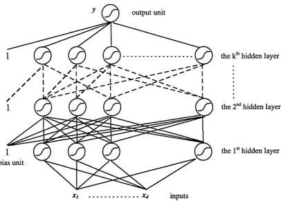
popular type of ANN. Backpropagation networks are multi-layer feed-forward

networks that use the backpropagation algorithm [Wer74] [Par85] [leC85] [Rum86c]

for training. A BPN, as shown in figure 1.2, consists of multiple layers of sigmoidal

units (that is, processing units with a ‘S ’-shape transfer function). Adjacent layers are

fully connected and there is no loop-back connection to lower layers. Like other

nonlinear feed-forward networks, the outputs can be expressed as deterministic

functions of the inputs and the whole network represents a multivariate non-linear

mapping.

Figure 1.2 A typical backpropagation network. Note that the output layer can have more than one unit although only a single unit is shown. Also, the hidden layers are not restricted to have

the same number of units.

The original backpropagation algorithm uses a sum-of-squares error function and simple

gradient descent for optimization. Training consists of iterating two distinct stages: a

forward propagation of the activation generated by the inputs through the network, and

the backward propagation of the error signals and the adjustment of weights. The

backward propagation of errors allows the derivatives of the error function with respect

[image:23.531.77.484.243.534.2]

(24)

also reduces the computational complexity in evaluating the derivatives from 0(W~) to 0(W) where W is the number of adjustable weights.

Backpropagation is of great practical importance because of its simplicity and its

efficiency. Backpropagation can be used in many other types of networks apart from

multi-layer feed-forward networks. It can also be applied to other error functions and

use a variety of optimization schemes. As long as the transfer function of the processing

units are differentiable in their inputs and parameters, the use of sigmoidal units is also

not essential.

2

1.3.3 RBF Networks (RBFN)

Kriging is closely related to an ANN architecture known as radial basis function

networks [Bro88], [Moo89b], [Pog90]. The close relationship between the two has

been examined by Wan and Bone [Wan96]. In [Wil96], W illiams and Rasmussen have

also indirectly linked kriging to regularization networks (RN)7 - a special class of RBFN

that can be derived from regularization theory [Pog90].

linear output unit

output weights

hidden RBF units

inputs

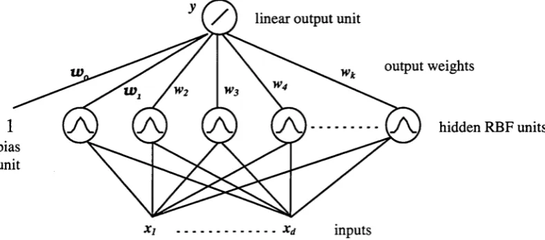
Figure 1.3 A standard radial basis function network. Note that the output layer can have more than one unit.

7 Williams and Rasmussen linked both kriging and regularization networks to Gaussian process prediction. However, they rather inaccurately referred to kriging as ‘Gaussian processes ... used in the geostatistics field’. In fact, the formulation of kriging is not based on a Gaussian process framework. Kriging is derived as the optimal unbiased linear predictor that gives the minimum error variance

[image:24.531.66.461.442.616.2]

(25)

A standard RBFN, as shown in figure 1.3, is a two-layer feedforward network and

consists of a single hidden layer of RBF units or nodes - units whose transfer functions

are radial basis functions - and a layer of linear output units. Typically, a bias unit is

also connected to each output unit. The role of the bias units are to compensate for the

difference between the mean of the network outputs and the mean of the target outputs

over the training set8. The parameters of the RBF units - their locations and widths - are

pre-specified or set by unsupervised methods or some simple heuristics. The output

weights between the output units and the hidden units (including any bias units) are then

optimized by supervised training with the parameters of the RBF units fixed. The

optimization involves solving a linear problem and is very fast.

Hartman, Keeler and Kowalski showed that Gaussian RBFNs are universal

approximators, that is, they can approximate any continuous function to any accuracy

provided that there are enough hidden units [Har90]. Park and Sandberg extended the

results to other classes of radial basis functions and showed that with some mild

restrictions on the form of the RBF functions9, the universal approximation property

still holds [Par91].

The regularization networks are special RBFN. More specifically, a regularization

network has as many RBF units as there are data points with each RBF unit located at

one data point. The radial functions used by the RBF units are identical and satisfy

certain smoothness condition imposed by a smoothness regularizer. Like splines,

regularization networks also use a smoothing parameter to control the trade-off between

data misfit and smoothness. In fact, splines are special regularization networks.

The standard RBFN model [Bro88] [Moo89b], differs from RBF interpolation in the

following ways [Bis95]:

1. The number of RBF units can be much smaller than the number of data points;

2. The locations of the RBF units are not constrained to those of the data points;

(26)

3. The RBF units can have different widths;

4. The addition of the bias units to offset the network outputs is allowed.

Hence, in general, RBFNs as well as regularization networks are not exact interpolators. However, like RBF interpolation and splines, the class of the radial function is pre specified a priori while the parameters of the basis functions are set by some more or less ad hoc procedures. Hence, as in the case of RBF interpolation and splines, the radial function used may be in conflict with the actual covariation in the data. To match the covariation in the data, non-linear optimization of the parameters of the radial basis functions are required and the generalized RBFN (GRBFN) [Pog90] has to be used.

1.4 The Goals of this Thesis

The three main goals of this thesis are to:

1. investigate the formal relationship between kriging and neural networks - more specifically, between kriging and RBF networks,

2. apply neural network techniques to solve the variogram model fitting problem, and

3. apply neural network techniques to solve the local stationarity problem.

Current BPN approaches to ore reserve estimation have not gained wide acceptance among practitioners and geostatisticians. The major problem in using BPN has been the difficulty in specifying an appropriate model of the data to constrain the solution. It is equally difficulty to extract information about the model learned by the BPN in order to validate the method. Kriging, on the other hand, has been extensively studied and is well accepted by the geostatistics community. However, no serious attempt has been made to examine whether there exists a formal equivalence between kriging and any type of ANN. The availability of such a formal relationship provides a strong

(27)

foundation and justification for developing and applying ANN techniques for interpolating earth-science data.

From the ANN perspective, a formal relationship between the kriging and RBFN offers an alternative interpretation of the parameters of RBFN. At the moment, Gaussian units have been used almost exclusively. In addition, the widths of the RBF units have typically been determined by more or less ad hoc heuristics. This thesis sheds some light on how the class and the parameters of the radial basis function of an RBFN can be selected for the class of problems where a spatial model is appropriate.

An equivalent or approximate RBFN implementation of kriging inevitably means inheriting the problems of kriging. For optimal prediction, the parameters of the kriging model have to reflect the trend and the covariation in the data. In other words, the prediction accuracy will suffer if the RBFN’s parameters are set to values that are in conflict with the trend and the covariation in the data. Current geostatistical solutions to the critical problems of local stationary and variogram model fitting are far from satisfactory.

In this thesis, we propose using MacKay’s evidence procedure IMac92] - an empirical Bayesian approach - to estimate the parameters of the ‘kriging’ RBFN. The evidence procedure has been applied successfully in image reconstruction [Gul89] [Wei91] and in neural networks [Mac92] [Tho93] [Mac94a]. While the connection between the

(28)

To solve the local stationarity problem, we propose using a hierarchy of GRBFN to soft partition the input space into spatially correlated regions, learn the local covariation models and combine the predictions of the local GRBFN experts. The approach is based on the idea of hierarchical mixtures o f expert (HME) [Jac91 ]. We suggest extending the original expectation-maximization (EM) training algorithm of HME [Jor94] to include priors on the parameters of the experts in order to improve generalization. The architecture of HME and the extended training algorithm are described in Chapter 6.

Our neural network approach allows the initial partitioning of the input space and model fitting as well as the subsequent interpolation to be performed within the same general framework. In geostatistics, these problems are tackled separately at different stages in different frameworks. At each subsequent stage, the results of the previous stages are treated as perfectly known. The use of a single neural network framework as developed in this thesis opens up the possibility of adjusting all the interdependent factors involved in the various stages of the kriging process simultaneously to achieve the single ultimate goal of optimal prediction.

1.5 Related Works

Neural network approaches are only recently starting to get some attention in the field of applied geostatistics, and their use is largely on classification tasks. Only a handful of researchers have used ANN for reserve estimation, and that the effort has been confined to the use of backpropogation networks.

(29)

Instead of using a single network, Denby and Burnett [Den95] divided a mineral deposit into smaller rectangular overlapping zones, and used each zone to train a small BPN. Predictions of the networks over the overlapping areas were then averaged to obtain the final predictions. Denby and Burnett’s approach effectively used a local training

algorithm and combined multiple (local) predictors to reduce the variance of the prediction (over the ensemble of possible training data). Like Wu and Zhou, they also employed a network construction scheme to incrementally increase the size of the hidden layers of the BPNs. They reported predictions close to the kriging predictions on the data sets they tested.

1.6 Reasons for Using RBFN and not BPN

The arguments propounded for using BPN are mainly:

1. They have been successfully applied to other similar real world problems such as image processing and time series modeling and that they have been proved to be a universal approximator [Hor89].

2. It is a model-free approach. No complicated mathematical model and no

assumption about the statistical distribution of data are required. Consequently, the technique is general, robust and applies to all data sets.

3. Its is capable of uncovering the underlying statistical properties (including the spatial structures) in the data, learning the input/output relationship and then generalizing to new data.

4. The flexibility of the representation scheme makes it possible to include inputs other than the geographic locations of the data without changing the technique [Den95].

(30)

dedicated to a particular class of solutions. Nevertheless, for any fixed architecture, minimization of the particular error function is not over all possible functions, but over the class of function generated by all allowed values of the network weights.

Without the constraints of a data model, both Wu and Zhou as well as Denby and Burnett attempted to use a network construction algorithm to limit the capacity of the BPN so that it generalizes better. However, their stopping criteria was based on the training error which is not a good estimator of the generalization error. A separate validation set can also be used for estimating the generalization error. However, apart from its dependence on the distribution of the data in the validation set, the requirement of setting aside a separate set of data is unattractive because of the often limited amount of data.

Unlike BPN, RBFN can be derived using a regularization approach. The regularization approach introduces an additional term to the cost function to constrain the value of the network parameters. In chapter 4, we further show that the smoothness regularizer of RBFN can be viewed as enforcing a covariation model of the data.

The regularization approach can also be used with BPN. The most common regularizers for BPN are weight decay10 [Hin87] which favors small weights, and

weight elimination [Wei90] which favors large weights. A more complex form of regularization known as soft weight sharing [Now92] divides the weights into groups whose mean values and spreads are determined as part of the training. Recently, Moody and Rögnvaldsson derived a family of regularizers which bound the corresponding regularizers of splines of various degrees11 [Moo97]. These regularizers represent different prior assumptions on the distribution of the weights and correspond to different model assumptions. However, all except Moody and Rögnvaldsson’s regularizer of BPNs have no obvious physical interpretation. Even Moody and Rögnvaldsson’s smoothness regularizers correspond approximately to a specific family of covariation models - those of splines - at best.

(31)

In summary, while the RBFN model is consistent with the kriging model and has a sound physical interpretation, there is a lack of knowledge on the implicit constraints of BPN and on the physical interpretation of the additional constraints commonly imposed on its parameters. In addition, a ‘model-free’ approach such as BPN performs best in a

‘data-rich’, ‘theory-poor’ situation [Gem92] [Rum95]. In view of the sparse sampling that is typical of many earth-science problems, it is questionable whether a BPN is able to provide good generalization without the explicit constraints of a reasonable model.

Nevertheless, it should be noted that the linear kriging predictor and hence its equivalent RBFN is only optimal for Gaussian processes. If the geophysical process is non-

Gaussian, given sufficient data, it is possible that the BPN approach may uncover a non linear mapping that better describes the data and leads to more accurate prediction.

1.7 Thesis Outline

In chapter 2, the mathematical model and formulation of kriging will be presented. The various measures of spatial continuity and the common variogram models will be briefly discussed. In chapter 3, Poggio and Girosi’s regularization approach to RBFN [Pog90]

will be briefly described. The computation of the GRBFN parameters using the evidence procedure - an empirical Bayesian approach - of MacKay [Mac92] will be developed. Chapter 4 will examine the close formal relationship of kriging and GRBFN and the different data models used by the two approaches. A GRBFN approach to variogram model fitting and the interpolation of sparse earth-science data will be developed. In chapter 5, the effectiveness of the approach will be demonstrated by its application to simulated data sets. In chapter 6, the mixtures of experts (ME) [Jac91] and its hierarchical extension, hierarchical mixtures of experts (HME) [Jor94], will be briefly described. The GRBFN approach of chapter 4 will be extended to use a

(32)

(33)

2. Kriging: An Overview

Kriging is an interpolation method widely used in the earth-sciences for spatial

prediction. Spatial prediction is ‘the prediction of unobserved values from observed

data for which the only exogenous variables are their spatial locations’ [Cre93]. The

kriging approach uses a spatial model which specifies the large- and small-scale spatial

variability in the data to derive the optimal unbiased linear predictor for unsampled

locations. The predictor is optimal in the sense that it minimizes the error variance.

There are two main advantages of kriging over other commonly used deterministic

predictors such as moving average and inverse-distance-squared weighted average.

Firstly, it takes into account the spatial dependence demonstrated in the data. Secondly,

it provides a confidence measure, the kriging variance, for the predicted value.

Nevertheless, the spatial variability in the data is in general unknown and a model has to

be estimated from the data by an initial structural analysis. Typically, a low order

polynomial is specified to characterize the slowly varying trend of the data. The

analysis then fits a covariation model to a spatial continuity measure of the detrended

data either graphically or by means of various least squares (LS) methods. Maximum

likelihood (ML) approaches which estimate the covariation model directly from the data

have also been used.

There exist a number of variants of (univariate) kriging. The most commonly used are

universal kriging, ordinary kriging and indicator kriging. Ordinary kriging is actually a

special case of universal kriging while indicator kriging is just the (universal or

ordinary) kriging of binary indicators at specified thresholds. In addition, multivariate

(34)

In this chapter, the commonly used variogram models and model fitting techniques will be briefly described, and a short overview of the mathematical formulation of four types of kriging: universal kriging, ordinary kriging, indicator kriging and cokriging, will be presented.

Special emphasis will be given to universal kriging as, in this thesis, we are mainly concerned with equivalent neural networks implementations of universal kriging and ordinary kriging as well as their approximations. In addition, without loss of generality and for the sake of clarity, ordinary kriging will be used in the experiments in later chapters. Indicator kriging involves an initial transformation of the real sample data to binary indicators and the subsequent kriging of the indicators. Hence, the neural network approach developed in the thesis can be readily extended to indicator kriging.

Cokriging and local kriging will be briefly described in this chapter while their equivalent neural network implementations will be discussed in chapter 4. Trend- surface prediction will also be briefly described because it can be viewed as a special case of universal kriging that uses the same data model used by most neural networks for interpolation tasks.

The probabilistic approach to kriging is but one way to achieve the goal of minimizing the average squared prediction error. JoumeTs deterministic version of kriging will be briefly discussed because it gives a more concrete interpretation to the otherwise elusive notion of the covariation model and helps to reconcile the differences between the probabilistic model of kriging and the deterministic models used in most neural network approaches.

2.1 The Spatial Model

Let the observed data within an area A be D = {(x(,),y (,)}/ = l,...,n} where x0),s are

(35)

Let the random process be {k(x)x e A}. T(-) is considered to be made up of two

components:

F(x) = /i(x) + <5(x), x eA, (2.1-1)

where //(•) is the deterministic trend which captures the large-scale structural variation while $•) is a zero-mean, stationary stochastic residual (or error process) that captures the small-scale variation. The residual is assumed to be either intrinsically or second- order stationary.

Definition 2.1: For a random process Z(-), intrinsic stationarity means that the expected value of Z(-) is independent of its location, that is, £(Z(x+h)) = £(Z(x))), and the variance of the first difference of Z(-) at any two locations is a function of the displacement (or lag) between them, that is, var(Z(x+h)- Z(x)) = 2}{h) for some function y

Definition 2.2: For a random process Z(-), second-order stationarity means that the mean and the covariance of Z(-) are both location invariant, that is, E(Z(x-i-h)) = E(Z(x)) and cov(Z(x+h), Z(x)) = C(h) for some function C.

As explained in section 1.1.1, the trend/residual decomposition is not unique and is largely subjective. It depends on the application and the experience of the modeler. In this thesis, we will not concern ourselves with the non-uniqueness of the decomposition. We are interested in developing neural network approaches to learn model parameters that produce accurate predictions once a spatial model is specified.

2.2 Covariation Modeling

Before kriging the data, a covariation model has to be estimated from the data to

(36)

(or correlation function)1, with the variogram being the most commonly used. A variogram model is fitted to the sample variogram estimated from the data. For a second order stationary process, the variogram can be converted to the corresponding covariogram and correlogram using the relationships:

2y(h) = 2 ( c ( 0 ) - C ( h ) ) and (2.2-1)

p(h) = C (h )/C (0 ) (2.2-2)

where 2X0 is the variogram, C(-) is the covariogram and p(0 is the correlogram. Note that, traditionally, the variogram is denoted as 2X0 while XO is referred to as the

semivariogram. It should be pointed out that the above relationships only hold for the probabilistically defined functions XO , C(0 and p(-), and are not necessarily valid for their corresponding estimators.

The use of a variogram implies that the process to be modeled is intrinsically stationary while covariogram and correlogram only exist for processes that are second-order stationary which is a stronger assumption than intrinsic stationarity. However, which assumption should be used is more or less a matter of taste as most of the commonly used covariation models satisfy the stronger assumption of second-order stationarity. Most practitioners are more familiar with covariance functions and prefer to work with them. Traditionally, variograms have been used for fitting covariation models. Often, the fitted variogram model is then converted to the corresponding covariance function for subsequent analysis and computation using the relationship (2.2-1).

2.2.1 Variogram

The variogram value at lag (or displacement) h, 2}(h ), is defined as the variance of the squared differences between pairs of points that are a displacement h apart

2r(h)=var(r(x + h )-r (x )) (2.2-3)

(37)

When the random process is stationary, the mean of the differences is zero and the

variogram equals the average of the squared differences. Hence, the variogram

measures the rate of change of a random variable along a specific direction.

The classical estimator of the variogram proposed by Matheron [Mat62] is

2 r( h ) = p ^ I (y(x<'>)-y(xM))2 (2.2-4)

( i j ) e N (h)

where /V(h)= j(i,i/ ) x (,) = hj and |w(h)| is the number of sample pairs included

in the calculation. In practice, only a small number, or even no sample pairs will be

exactly a lag h apart, pairs whose displacement are within a certain tolerance of h have

to be included in the summation. The tolerance region should be as small as possible to

retain spatial resolution but large enough so that the estimator is stable. Joumel and

Huijbregts have recommended that there should be at least 30 distinct pairs for each lag

h [Jou78].

range, a

[image:37.531.122.411.431.598.2]

nugget variance, b0

Figure 2.1 A generic semivariogram

Figure 2.1 shows a generic semivariogram. At lag 0, each sample point is being

compared with itself and }{0) is strictly zero. For small lags, the samples being

compared tend to be very similar, and Xh) are relatively small. However, factors such

(38)

value of zero at the origin of the semivariogram - a feature known as the nugget effect

which is modeled by a white noise process. The corresponding semivariogram value is known as nugget variance. As the lag increases, the samples being compared are less and less related to each other, resulting in larger ^h). At some distance, the range, the samples being compared are so far apart that they are not related to each other, }{h) approaches the variance of the random variable. Beyond the range, ){h) no longer increases, the semivariogram develops a flat region called the sill.

2.2.2 Variogram Model

In practice, the variogram values are calculated using a variogram model. The

variogram model is chosen by fitting an appropriate function to the sample variogram calculated directly from the sample data. For the following discussion, we need the following definitions:

Definition 2.3: Let Rd be the ^-dimensional Euclidean space. A symmetric, real-valued function G(s, t) where s, t e Rd is said to be positive definite and negative definite on Rd

if, for any real vj, ..., v„, and xi, ..., x„ e Rd, the quadratic form vTGv > 0 and vTGv < 0 respectively, where v = [vj, ..., v„]T and (G)ij= G(x„ xj).

Definition 2.4: Let Rd be the d-dimensional Euclidean space. A symmetric, real-valued function G(s, t) where s, t e Rd is said to be ^-conditionally positive definite (or

conditionally positive definite of order k) and ^-conditionally negative definite (or conditionally negative definite of order k) on Rd if, for any real vj , ..., v„, and Xj, ..., x„

I 'T' >-p rT

e R such that v [/?(xi), ..., p(xn)] = 0 where v = [vj, ..., v„] t for all polynomials pof degree at most k-1, the quadratic form vTGv > 0 and vTGv < 0 respectively, where (G)ij

= G(Xi, xj).

(39)

well-defined, the variogram function has to be 1-conditionally negative definite. If the

covariance function is used, it has to be positive definite. This means that one cannot

obtain such a function by simply interpolating between the sample variogram values.

Variogram models are usually constructed by linearly combining with positive

coefficients a few simple radial basis functions which are valid variogram models

themselves.

The most commonly used isotropic basis semivariogram models in applied geostatistics

are:

• the spherical model:

0,

r M ) = k +i1{|(J?)-i(1!1)2

3}, o < Ml

h = 0

< a

iA)+V

i h > a

(2.2-5)

where 9 = [b0,b] ] with the nugget variance b0 > 0, the magnitude of the

spherical component > 0 and the scaling parameter a > 0;

the exponential model:

r (h ;0 )

0, h = 0

b0 + b{s\ - e a X h ^ 0 (2.2-6)

where Q = \b0,bl , a j , b0 > 0 , bx > 0 and a > 0; and to a lesser extent

2.

the power model*":

y (h ;9 ) = JO, h = 0

K + I - W T . h^O (2.2-7)

(40)

where 0 = [b0, m , p j with b0 > 0, the slope m > 0 and the power 0 < p < 2.

2.2.3 Anisotropy

In case of geometric anisotropy where the range changes with direction, the anisotropy

axes that correspond to the minimum and maximum range have to be first identified.

Graphically, contour maps of the variogram surface can be used to determine these

directions. A more commonly used alternative is to plot the ranges for a number of

directional sample variograms as solid lines (whose lengths are proportional to their

values) at their corresponding orientations on a number of rose diagrams (figure 2.2). With 3D-data, the computation and comparison of a series of rose diagrams can become

[image:40.531.129.379.325.569.2]

a very tedious and error prone exercise.

Figure 2.2 A rose diagram of the ranges of nine directional sample variograms whose directions lie on a 2D plane. The thin solid lines show the ranges of the directional sample variograms as well as their orientations. The dotted line is the contour of the range of the fitted

anisotropic variogram model.

The anisotropy axes are usually modeled as mutually perpendicular. The anisotropic

model with the same types of basic models in the directional variogram models can be

(41)

system by pre-multiplying the lag vector with an appropriate scaling matrix S and a

rotation matrix R. That is, the transformed lag vector h is given by:

h* = S R h .

In the 3D case, traditionally S and R is specified as:

a x 0 0

s = 0 J _f l y 0

0 0 J_

a : _

(2.2-8)

(2.2-9)

R - R yR xR z

c o s(a v) 0 sin (« v) 1 0 0 cos(a; ) - sin ( a . ) 0 0 1 0 0 cos(«v) - s i n ( a r ) s in (a .) c o s (a .) 0

- sin(erv) 0 cos(«v) 0 sin (a t ) cos(ax) 0 0 1

(2.2-10)

where az is the azimuth angle measured clockwise from the y-axis of the coordinate

system (which points to the north) to the maximum range direction, ax is the dip angle

measured in negative degrees from the horizontal down to the maximum range

direction, and ay is the angle (measured clockwise) that is required to rotate the z- and

x-axes to the two directions orthogonal to the maximum range direction once the y-axis

has been rotated to the maximum range direction (figure 2.3). The anisotropic

variogram model can then be evaluated using the isotropic variogram model and the

(42)

[image:42.531.132.424.53.289.2]

Figure 2.3 The three angles which define the orientation of the anisotropy. The direction of y’ denotes the maximum range direction. The ellipse shown is the contour of the range of the anisotropic model at the model’s x’y’ plane. The shaded portion of the ellipse is the part of the

ellipse that is below the horizontal plane xy of the coordinate system. Rotation through the three angles (X -, a x and a y are known as azimuth, dip and plunge corrections respectively in

geology.

2.2.4 Fitting a Variogram Model

Most practitioners fit the postulated variogram model to the sample variogram "by eye", or by ordinary least squares (OLS) through a selected subset of the sample variogram values. A number of automated and more objective fitting methods have been