R E S E A R C H
Open Access
Joint integrated track splitting for
multi-path multi-target tracking using OTHR
detections
Yuan Huang
1†, Taek Lyul Song
1*†and Joo Hyun Lee
2Abstract
In target tracking applications where an over-the-horizon radar (OTHR) is used to gather measurements, one target may generate more than one measurement at each scan due to the multi-path propagation effect. However, traditional tracking methods obtain the data association probabilities based on track-to-measurement data
association events under the assumption that each target can generate at most one detection at each scan, leading to poor performances if these methods are applied to multiple detection applications such as OTHR applications. In this paper, we develop a multi-path multi-target tracking algorithm entitled multiple detection joint integrated track splitting (MD-JITS). This novel algorithm jointly solves the measurement origin uncertainty and measurement path model uncertainty. The probability of target existence (PTE) is utilized in the OTHR application as a track quality measure for true track confirmation and false track discrimination. The data association algorithm of MD-JITS the proposed algorithm is realized based on measurement cells that each measurement cell consists of one or more of the validated measurements, while considering the measurement path model. The proposed algorithm is compared with the multiple detection joint integrated probabilistic data association (MD-JIPDA) algorithm in a multi-target crossing scenario, implementing the OTHR system in the presence of clutter and failed target detections, to demonstrate the desired effectiveness.
Keywords: Multi-target tracking, OTHR, Multiple detection, Track management
1 Introduction
The core objective for the remote sensing target localiza-tion and tracking is to generate target state estimates using measurements processed by the sensors, such as the radar [1–3]. The measurements can originate from targets or from clutter and lead to both true tracks (following the tar-gets) and false tracks (following the clutter) existing in the surveillance area. Therefore, false track discrimination [4], involving true track confirmation and false track termina-tion, is crucial for tracking algorithms. The probability of target existence (PTE) was first introduced in [4] as a soft decision of the existence of a target, which can be used to alleviate the false track discrimination issue.
*Correspondence:[email protected]
†Yuan Huang and Taek Lyul Song contributed equally to this work.
1Department of Electronic Systems Engineering, Hanyang University,
Hanyangdaehak-ro, Ansan, Republic of Korea
Full list of author information is available at the end of the article
Most target tracking algorithms assume that the sen-sor can generate at most one detection per target with a detection probability (usually less than unity) at each scan
[5–10]. After the measurement selection procedure,
multi-target tracking (MTT) algorithms will generate the joint track-to-measurement assignments across the tracks. The main difference among the MTT algorithms lies in the way assignments are realized and how the corresponding probabilities are evaluated [11].
Among various MTT algorithms, the multiple hypoth-esis tracking (MHT) is a theoretically optimal track-ing algorithm that enumerates and evaluates all possi-ble track-to-measurement association hypotheses [5,12]. Each hypothesis represents a global association consid-ering all tracks and measurements over a number of scans. Based on the different hypothesis generation cri-teria, different versions of MHT can be divided into two
main groups. Measurement-oriented MHT [5] generates
hypotheses based on measurements, while track-oriented
MHT [12] generates hypotheses based on tracks. The maximum likelihood probabilistic multiple hypothesis tracking (ML-PMHT) is a powerful non-Bayesian algo-rithm that uses a generalized likelihood ratio test to confirm target existence [13]. Ciuonzo and Horn [14] use a Merkle tree to store and organize hypotheses for a distributed track-oriented multiple hypothesis tracking (TO-MHT) resulting in an efficient structure for imple-mentation.
The joint integrated probabilistic data association (JIPDA) tracker is a single-scan MTT algorithm that incorporates the probability of target existence into the JPDA algorithm as a track quality measure [15]. JIPDA is widely used mainly because it is easy to implement and has low computational cost, due to how all the data asso-ciation events for a track are compressed into one track state at each scan. In the JIPDA framework, the proba-bility of target existence is used to solve the false track discrimination problem, and the track state is generated under the assumption of target existence. Compared to the multi-scan global hypothesis generated by the MHT tracker, the JIPDA forms track-to-measurement data asso-ciation events based only on current scan circumstances, which significantly lowers the computational expense. As suggested in [12], under adverse circumstances, especially when the clutter density is high and the detection proba-bility is low, JIPDA may have poor tracking performances. In [16, 17], the maximum likelihood probabilistic data association (ML-PDA) algorithm is utilized to identify the sensor states as well as target states.
The joint integrated track splitting (JITS) algorithm is a multi-scan MTT tracker [11]. Each track generates a hypotheses tree consisting of a set of hypotheses. Each hypothesis is treated as a track component, representing one assertion of the possible target detections history for multiple scans. Every component selects measurements and spawns new components, and these new components propagate to the next scan. The track state is updated by a Gaussian mixture of all the components belonging to that track. The probability of target existence is an inher-ent part of the tracking state and is recursively updated based on the measurement likelihood ratio, considering all the components. Updating the estimated state and the probability of target existence are two core aspects of JITS. As the number of hypotheses exponentially grows, component reduction methods are used. Pruning and merging are the efficient and most widely used methods [18,19] for controlling the number of components. Both JIPDA and JITS use the probability of target existence to solve the false track discrimination issue, and the com-parison results showed that JITS outperforms JIPDA at the expense of computational complexity [11]. Instead of the global hypotheses being generated by the MHT, JITS forms a hypotheses tree for each track, which significantly
reduces the structure complexity. Some of the differences and tracking performance comparisons of IPDA, ITS, and MHT are shown in [20]. Kim and Song [21] proposed the smoothing JITS for multi-target tracking in clutter.
These algorithms assume that for each scan, one tar-get can give rise to at most one detection with a given detection probability of PD < 1. However, many
prac-tical applications are plagued by the multiple detection problem. This problem is especially prominent when a special kind of radar, called the over-the-horizon radar (OTHR) [22–24], is used. In [22–24], the multi-path prob-abilistic data association (MPDA) method is introduced for single-target tracking. However, the multi-path tracks are generated as it lacks a means of discrimination. In the OTHR tracking system [25–28] which is widely used in remote sensing applications, transmission and receiv-ing signals can be scattered by different ionospheric layers which results in different measurement paths (models). The multi-path approach leads to multiple detections gen-erated by the same target, and the relationship between measurements and paths is not prior known which results in the measurement path model uncertainty. If the tar-gets in the surveillance region are closely spaced and cross each other, localization and tracking become more diffi-cult. Moreover, due to the incorrect model and measure-ment combination, multi-path tracks are generated and need to be identified. In [25,27], the multiple detection multiple hypothesis tracking (MD-MHT) algorithm and the multi-detection probability hypothesis density (MD-PHD) algorithm are derived by combining the multiple hypothesis tracking and the random finite set frame-work. In [29], the Gaussian mixture probability hypothesis density (GM-PHD) filter is extended for path multi-target tracking with the over-the-horizon radar system. But the MHT and the PHD algorithms lack a specialized track quality measure for true and false track manage-ment. In [26,28], the Bernoulli filter and the cardinality balanced multi-target multi-Bernoulli filter are applied to the OTHR applications. However, the Bernoulli filter-based methods are recommended to use in the envi-ronment with high detection probability and low clutter density. In [30], the authors developed the multi-radar multi-target tracking algorithm for maritime surveillance at over-the-horizon (OTH) distances.
in one date association event, the tracking performance can be improved significantly due to the target informa-tion being more efficiently extracted. The measurement partition method is introduced to generate the possi-ble target-oriented measurement cells and was embedded
in the JPDA and PHD frameworks [27, 31]. The
mea-surement partition method assumes that more than one measurement can be generated by one target, forming all the possible target-oriented measurement combina-tions based both on the validated measurements and on the restriction of the maximum number of target detec-tions. Those measurement cells are then used in the data association events instead of a single measurement. The algorithms in [27, 31] are multi-target tracking meth-ods but do not have the track quality measure which is essential for distinguishing true and false tracks.
Both JIPDA and JITS assume that at most one mea-surement per target at each scan, which leads to infor-mation loss in multiple detection scenarios. By jointly considering the measurement origin uncertainty and the measurement path model uncertainty, two novel struc-tures named multiple detection JIPDA (MD-JIPDA) and multiple detection JITS (MD-JITS) are designed espe-cially for use in the OTHR tracking system. In these two multiple detection structures, after the measurement selection step, the measurement cells are first generated such that one measurement cell may contain one or more of these validated measurements. Then, the data associ-ation events of MD-JIPDA and MD-JITS are generated using the measurement cells. Combined with prior infor-mation from the last scan, the measurement cells are used to update the track state and the probability of target existence.
The track state of MD-JIPDA is generated by a Gaus-sian mixture based on all the data association events, and then, this track propagates to the next scan. The output of MD-JIPDA for each track at each scan contains one Gaussian distribution for the track state and the proba-bility of target existence. As for MD-JITS, at each scan, each component selects measurements and generates the measurement cells separately. Each component generates new components using any one of its own measurement cells, where each component is represented by a Gaus-sian distribution for its state and a component probability. The final output for the track state is obtained by a Gaus-sian mixture based on all the components that belong to the track. Then, the components of the track propa-gate to the next scan where each component can be seen as a measurement cell assignment history. Compared to MD-JIPDA, in which each track propagates as one Gaus-sian pdf, each MD-JITS track propagates as a set of many Gaussian components. The number of components of a track exponentially increases with the number of scans, but actually not all the components are significant for the
track. Thus, the components with the component prob-abilities lower than a given threshold are pruned, and if any two components consecutively use the same mea-surement cells to update the component states for several scans, these two components should be merged into one [18, 19]. Since the MD-JITS track maintains many track components which can be seen as the target-generated measurement hypotheses, it outperforms MD-JIPDA in the multi-target crossing scenarios.
Initial results of MD-JITS are reported in [32] in
which the multiple detection problem occurs from a high-resolution sensor. The algorithm proposed in [32] only needs to solve the many-to-one measurements-to-track associations. However, in order to associate mul-tiple measurements to one track, the work proposed here should jointly consider the measurement origin uncertainty and the measurement path model uncer-tainty caused by the unknown signal propagation paths of the OTHR. The same measurement with different measurement path models provides completely different target state information. We provide here the rigorous algorithm derivations of MD-JITS for the OTHR sys-tem by utilizing the combinations of the measurement cells and the path models. We also introduce a multi-path track discrimination method for the data association structures.
The problem statement is given in Section2. The math-ematical derivation of MD-JITS for the OTHR system and the complexity analyses are given in Section3. Section4 contains the simulation studies, followed by conclusions in Section5.
In this paper, the following abbreviations, notations, and the assumption are employed:
A. Abbreviations:
CFT: Confirmed false tracks; CTTs: Confirmed true tracks; EKF: Extended Kalman filter; JIPDA: Joint inte-grated probabilistic data association; JITS: Joint inteinte-grated track splitting; MD-JIPDA: Multiple detection joint inte-grated probabilistic data association; MD-JITS: Multi-ple detection joint integrated track splitting; MD-MHT: Multiple detection multiple hypothesis tracking; MD-PHD: Multi-detection probability hypothesis density; ML-PDA: Maximum likelihood probabilistic data association; ML-PMHT: Maximum likelihood probabilistic multiple hypothesis tracking; MPDA: Multi-path probabilistic data association; MHT: Multiple hypothesis tracking; MTT: Multi-target tracking; OTHR: Over-the-horizon radar; PTE: Probability of target existence; RMSEs: Root mean square errors
B. Notations:
χt
k The event that tracktis tracking a target i.e., targett
exists.
t,max The maximum number of target originated
measurements in the mk validated measurements,
t,max=min(L,mk).
zt,nt(k) One measurement cell of tracktat timek.
t The number of measurements originated from target
tsuch that 1≤t≤t,max.
nt An index that indicates is the measurement cell
zt,nt(k) is one of the possible ct combinations
where there aret measurements originated from
target t. nt ∈
1, 2,. . .,ct
and ct = C
mk t = mk!
t!(mk−t)!(the notationC n
min this paper represents
the number ofm-combinations from a given set ofn elements).
z(k) The measurement set that of all the
val-idated measurements at scan k, z(k) =
z1(k),z2(k), ...,zmk(k)
.
Zk A collection of validated measurement sets that
includes all the validated measurements up to and including scank,Zk =z(k)Zk−1.
The superscript or subscripttindicates that the param-eter is specified by trackt.k always represents the time index.
C. Assumption:
There areLmeasurement paths, and each target can be detected at most one time through each of those paths.
This suggests that there are at most L target
measure-ments from each target at each scan.
2 Problem statement
The target motion model is given by
x(k)=f(k,x(k−1),v(k−1)). (1)
Here,x(k)represents the target state at scank,f is the state propagation function, and v(k−1) is the process noise.
In the OTHR system, the high frequency wave reflects through ionospheric layers to detect a target located beyond the horizon. The signal is emitted by the transmit-ter and reflected by one of the ionosphere layers before it reaches the target, and then, it is reflected by the target and bounces off one of the ionosphere layers before it is received by the receiver. Therefore, themdifferent iono-sphere layers formm2different measurement paths (mod-els). In order to demonstrate the measurement geometry and measurement generation process more concisely, only two ionosphere layers are considered in this paper. Here, two assumptions are made: one is the flat earth model and the other is that the heights of the ionospheric layers are known and fixed. Those two assumptions are employed in most OTHR studies [22,27,31] for simplicity. In order to consider the shape of the earth, the earth is introduced as an ellipsoid based on the WGS-84 coordinate system.
Then, the spherical OTHR measurement geometry can be modeled according to this coordinate system [33]. In realistic situations, the ionosphere state evolves intermit-tently. The noisy height information can be introduced by tacking into account that the ionosphere state changes slowly and stays invariable within the sampling period. Then, OTHR target tracking with the noisy ionosphere state is performed by joint estimation of fast-updating multi-target states and intermittent-updating the iono-sphere state [34–36].
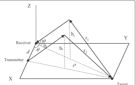
Figure 1 demonstrates the geometry of the planar
OTHR measurement model. The receiver is set as the ori-gin, and the transmitter is installed along theX-axis with
a distance d (T-R distance) away from the origin. The
targets move in the X-Y plane, and theX-Y-Z coordi-nate system follows the right-hand rule. The ground range between the target and the receiver is ρ, and the bear-ing between the Y-axis and ρ is defined as b. θ is the angle between theX-axis and the received signal satisfies cosθ = cosϕsinb, where the signal elevationϕ is not measured but has the relation cosϕ = ρ/(2r1)with the target stateρif the target statex(k)in (1) consists of the ground range, ground range rate, bearing, and bearing rate
x(k) = ρ,ρ˙,b,b˙T. The apparent azimuth is defined by
π/ 2−θ. The transmit and receive signals are reflected by the layers with heightshtandhr, respectively.htandhrare
used to represent the transmit layer and the receive layer, respectively. Half of the slant ranges from the transmitter to target, and from the target to receiver are denoted byr2 andr1, respectively.
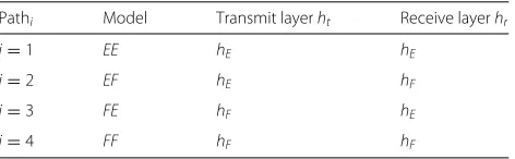
Here, two ionospheric layers are considered with verti-cal heightshEandhF.hEandhFare used to represent the
layerEand layerF, respectively. Under this circumstance,
the signal propagation models are shown in the Table 1
in which the height of the ionospheric layer is used to represent the layer.
Table 1Propagation models
Pathi Model Transmit layerht Receive layerhr
i=1 EE hE hE
i=2 EF hE hF
i=3 FE hF hE
i=4 FF hF hF
The measurements generated by the target and clutter are given by
zi(k)=
⎧ ⎪ ⎪ ⎪ ⎪ ⎨ ⎪ ⎪ ⎪ ⎪ ⎩
hEE(x(k))+wEE(k) model EE, Path1 hEF(x(k))+wEF(k) model EF, Path2 hFE(x(k))+wFE(k) model FE, Path3 hFF(x(k))+wFF(k) model FF, Path4
c clutter
(2)
wherehtr(t,r∈ {E,F}) is the measurement function
asso-ciated with the transmit layert and receive layer r. wtr
(t,r ∈ {E,F}) is the zero mean Gaussian measurement noise in the corresponding paths. Both htr andwtr are
related to the corresponding model.
The elements of each measurement consist of the slant range, the rate of change of the slant range, and the apparent azimuthRg,Rr,Az
[22], given by
Rg=r1+r2
Rr= ρ˙
4
ρ r1 +
η r2
,
Az=sin−1{ρsin(b)/(2r1)}
(3)
where the parametersr1,r2, andηare obtained by
r1=r1(ρ,hr)=
(ρ/ 2)2+h2r
r2=r2(ρ,b,hr)=
(ρ/ 2)2−dρsin(b)/ 2+(d/ 2)2+h2t η=ρ−dsin(b),
(4)
wherehtandhr represent the height of transmit layer
and receive layer associated with different measurement models.
3 Multiple detection JITS
In the MD-JITS data association step, one has to con-sider the possibility that multiple measurements might originate from the same target. This special issue of the MD-JITS data association process involves jointly assign-ing the measurement cells to the tracks. At each scan, each component of each track employs the gating method [1, 2] to validate measurements. After obtaining vali-dated measurements, the measurement partition method
is used to generate the measurement cells from these vali-dated measurements. Each measurement cell contains one or some of the validated measurements. Then, a mea-surement cell assigned to a tracker should not share any elements with other tracks in a feasible joint event [3].
The joint events are used to jointly assign the measure-ment cells to the tracks, and each joint event is composed of tracks with disjoint measurement cells. In a joint event, each track is assigned to one measurement cell or unas-signed. Then, the joint event probabilities are calculated for the corresponding joint events.
3.1 Measurement partition method
In order to assign multiple measurements to one track, the measurement cells are generated. Each measurement cell can be treated as a measurement set which contains at mostt,maxelements of the validated measurements. In a data association event, if a measurement cell is assigned to a track, the measurements contained in this measurement cell are used for the state estimation and the data associ-ation probability calculassoci-ation. The measurement cells are generated using the validated measurements based on the
assumption that there are t measurements originated
from targett.
Here, we use an example to show the process of gen-erating the measurement cells. Suppose that trackt vali-dates three measurements{z1(k),z2(k),z4(k)}out of the total cluster measurements {z1(k),z2(k),z3(k),z4(k)} at scank,t,maxis set to be 3. Then, based on the assumed number of measurements from the target, measurement cells are generated as follows:
• Suppose that only one of the validated measurements is the target detection (t=1) andn1∈ {1, 2, 3}.
The measurement cells are:
z1,1(k)= {z1(k)}; z1,2(k)= {z2(k)}; z1,3(k)= {z4(k)}.
• Suppose that two of the validated measurements are the target detections (t=2) andn2∈ {1, 2, 3}. The
measurement cells are:
z2,1(k)= {z1(k),z2(k)}; z2,2(k)= {z1(k),z4(k)}; z2,3(k)= {z2(k),z4(k)}.
• Suppose that all these three measurements are the target detections (t=3) andn3∈ {1}. The
measurement cell is:
z3,1(k)= {z1(k),z2(k),z4(k)}.
utilized in the data associations for trackt. When mea-surement cellz2,2(k) is considered in a data association event, the measurements contained inz2,2(k), which are
z1(k)andz4(k), are treated as target detections.
The number of measurement cells increases with the
number of validated measurements mk and the
maxi-mum number of target originated measurementst,max.
After the measurement partition process, the number of
measurement cells becomest,max
t=1 C mk t.
Here, the measurement cells are generated without considering the measurement cell path model. The mea-surement cell path model, which contains path models for each measurement in the measurement cell, will be specified in Section3.2.
3.2 MD-JITS
When there are tracks that share measurements, the feasible joint events are used to solve the track-to-measurement assignment issue. The feasible joint events cover all possible track-to-measurement assignments for all the tracks and the measurements in a cluster. A cluster at scankis a set of the tracks and the measurements these tracks select. A track inside the cluster should share mea-surements with one or more different tracks in the cluster, and the tracks not belonging to the cluster do not select any of the cluster measurements. In the multiple detec-tion case, the measurement cells composed of different validated measurements are assigned to the tracks in one feasible joint event.
In this paper, for reasons of clarity and without loss of generality, it is assumed that all the measurements in the cluster are validated by all the tracks belonging to that cluster and that the detection probability of each path is considered identical, i.e.,PDEE=PDEF=PDFE=PDFF =PD.
MD-JITS is different from MD-JIPDA in the sense that each track in MD-JITS retains the track components for propagation. Denote by
composed of the t measurements of track t
gener-ated by a path model Mjt
t)! possible model path allocations. For
example, under the condition that L = 4 for the
measurement cell z2,2(k) = {z1(k),z4(k)}, the
corre-sponding measurement cell model Mtj
k means that measurementz1(k)is generated by path 3 and measurementz4(k)is generated by path 4 in Table1. In OTHR target tracking applications, the measurements are used with the specified path models since the same mea-surement with different path models provides different target state information.
Denote by
κt(k)= 0|0 (6)
the event that none of the validated measurements are the detections of targett.
One possible history of the validated measurement cells for tracktduring the interval between scan 1 and scankis represented by a set of events that represents a sequence of the measurement cells and the corresponding path model in the interval:
κt,k= κt(1)=z
Here, one recursion of MD-JITS at scan k is
illus-trated. At scan k, the following posterior information
at scan k − 1 is assumed to be available: (1) The
track state probability density function (pdf ) for track t, p
xt(k−1)|χkt−1,Zk−1
; (2) the probability of target
existence for trackt,Pχkt−1|Zk−1, which represents the probability of target existence of a target tracked by track t; (3) the component state for each component of trackt, pxt(k−1)|χkt−1,κt,k−1,Zk−1; and (4) the component probability for each component belongs to trackt, which isPκt,k−1|χk−1,Zk−1
.
The prediction and the measurement selection
pro-cesses are implemented by each component of track t.
where the Kalman filter prediction can be used for a linear state propagation model. Ifκt,k−1is omitted, this equation can be used for MD-JIPDA track state prediction.
The component probability prediction is given as
Pκt,k−1|χkt,Zk−1=Pκt,k−1|χkt−1,Zk−1; (9) the details can be found in [12,20].
The following describes the measurement selection of
each component of track t. Each component of track
t selects the measurements in its validation gate, and
all the components of track t form a common
valida-tion gate and common validated measurements of trackt [20,37]. Based on (8) and the selection process of the vali-dated measurements, each component of tracktgenerates
the predicted measurement for each measurement Pathi
and selects the measurements inside the validation gate corresponding to Pathiusing an ellipse gating method [3].
After selecting the measurements, the measurement partition for the set of validated measurements is applied to generate the measurement cells for possible multiple detection. Then, the component measurement cell likeli-hood function for each measurement cell is calculated as
pzt,nt(k)|χ
In (10), PG is the gating probability of a single
detec-tion. The Gaussian pdf for measurement cell zt,nt(k) is employed, and each measurement cell is allocated with one measurement cell path modelMjt
k
represents the measurement
prediction based on the state prediction (8) and
mea-surement cell path model Mtj
k
represents the measurement cell
innovation covariance corresponding to measurement cell zt,nt(k) given measurement cell path model
. One can apply the extended Kalman fil-ter (EKF) to obtain state estimates for the equations. The details for generating these estimates can be found in [22,23].
Equation (10) is the measurement cell likelihood func-tion calculated for each component. The combined mea-surement cell likelihood of trackt for measurement cell zt,nt(k) with allocated path model M the sum of products of the component measurement cell likelihood function and the component probability of the track components of trackt, written as
pzt,nt(k)|χ
where this combined measurement likelihood function utilizes all the components that use measurement cell zt,nt(k)with the allocated path modelM This combined measurement cell likelihood is used to calculate the joint event probability.
Then, the data association step is processed. In the following derivations, “track” and “measurement” mean cluster tracks and cluster measurements in a cluster, respectively. The validated measurement set z(k) is the union of the validated measurements validated by each of the tracks belonging to the cluster. A joint eventεis an event of assigning measurement cells including non-detection to all the tracks. One joint event should sat-isfy the following: (1) Each track is assigned to at most one measurement cell and (2) each measurement cell is assigned to at most one track.
To generate the a posteriori probability of the joint event
ε, the tracks are divided into different sets.Tεis the set of tracks that are assigned a measurement cell, and the num-ber of tracks in this set isNε.T0ε is the set of tracks that are not assigned measurement cells (i.e., assigned to non-detection), and the number of tracks in this set isN0ε. The a posteriori probability of the joint eventε, using Bayes’ formula, is
where c is a normalization constant and mk is the
number of validated measurements in the cluster. pz(k)|ε,mk,Zk−1
is the joint measurement likelihood function for measurement set z(k); Pmk|ε,Zk−1
rep-resents the a priori probability for the number of the measurements; andPε|Zk−1is the a priori probability of the joint event.
The joint measurement likelihoodpz(k)|ε,mk,Zk−1
For the joint event ε, the relation between
measure-for every track involved in εis already known.
The number of clutter measurements follows a Pois-son distribution [38]. Givenmk measurements at scank, mk − N
ε
t=1t is the number of clutter-generated
mea-surements. The probability that mk − N
ε
t=1t clutter measurements are generated at scankis given by
P
where mˆk is the mean number of clutter measurements
such that mˆk = λVk with the clutter measurement
densityλ.
In (12), the a priori probability of the joint event εis given by
In (15), the a priori probability of the event that no vali-dated measurement is generated by targettincluding the hypothesis of non existence of targettat scankis
Pεkt,0|Zk−1=1−PtDecPχkt|Zk−1, (16) wherePχkt|Zk−1is the predicted probability of the exis-tence of targett. The probability that there is at least one target detection in the validation gate is given byPDec =
1−(1−PDPG)L.
In (15),Pχkt|Zk−1is the predicted probability of tar-get existence. The propagation of the probability of tartar-get existence for each target is modeled as a Markov chain [4,15]. The existence probability of targettand the non-existence probability at timekare denoted by Pχkt|Zk respectively. The Markov chain model defines two events
χt
kandχ¯ktby a random variableetksuch thatetk =1
repre-sentsχktandetk =2 representsχ¯kt. The predicted state of target existence from scank−1 to scankis given by
&
Equation (17) represents the prediction
pro-cess for the probability of target existence where Pij =P
etk =j|etk−1=i,j ∈ {1, 2}represents the transi-tional probability between the existence states.Pijsatisfies
2
j=1
Pij=1 fori∈ {1, 2}.
In (15), the a priori probability that the assignment is correct becomes
wherePDGtis the probability that there aret measure-ments detected and fall into the gate, given by
PDGt = probability of the joint association eventεas
Then, those joint events and the corresponding event probabilities are used to generate the data association probabilities of measurement cell-to-track assignments for MD-JIPDA and MD-JITS.
Denote by of all the joint events that allocate measurement cell zt,nt(k) to track twith measurement cell path model
. The probability that non-detection is assigned to tracktis the probability of the union of all joint events that assign non-detection to trackt, given by
Pκt(k)= 0|0 |Zk=
ε∈(t,0|0)
Pε|Zk. (21)
The probability that no measurement in the cluster is generated by targettunder the assumption that targett exists is given as
Pχkt,κt(k)= 0|0 |Zk with measurement cell path modelMtj
k
zt,nt(k)
is tar-gettdetection (detection of objecttimplies existence of objectt) is sive, and their union is the event of target existence. Therefore, the a posteriori probability of target existence is
denotes the summation through all feasible
joint events that contain the measurement cells with the allocated measurement cell path models of trackt includ-ing κt(k) = 0|0. The probability of non-existence Pχ¯kt|Zkis equal to 1−Pχt
k|Zk
.
The data association probabilities are given by
βt
So far, we have obtained the data association proba-bilities for track-to-measurement cell assignments for all the cluster tracks. In MD-JIPDA, each data association event generates one track a posteriori state pdf denoted by pxt(k)|χkt,κt(k),Zk, which can be obtained from the existing nonlinear filters, such as the EKF. The state for
tracktin MD-JIPDA is obtained by summing the
proba-bilities of all the data association events related to trackt under the assumption of target existence, given as
zt,nt(k)
,Zk−1 are presented in (10) and (11),
respectively.
The track state is updated using a Gaussian mixture of all the component state pdfs, given by
pxt(k)|χkt,Zk=
κt,k
pxt(k)|χkt,κt,k,ZkPκt,k|χkt,Zk, (30)
where pxt(k)|χkt,κt,k,Zk is the a posteriori state pdf for each component, which can be updated by the exist-ing nonlinear filters. If the EKF is used, the details to calculate the Jacobian matrix can be found in [22, 23]. Pκt,k|χkt,Zkis the a posteriori component probability, presented in either (28) or (29) depending on context. Equation (30) is different from Eq. (27) since the associ-ation history, which isκt,k, is considered in (30) and the association at current scan, which isκt(k), is considered in (27).
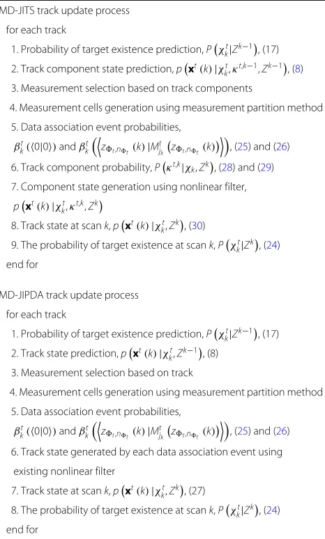
For comparison, the pseudo-codes for MD-JITS and MD-JIPDA are given in Table2.
3.3 Complexity analyses
Multiple detection multi-target tracking algorithms allow for many-to-one measurements-to-track assignments in the joint events. The number of feasible joint assignments (i.e., the number of the joint events) is combinatorial in the number of the measurements and the number of the tracks. In multiple detection multi-target tracking, most of the computational load is generated by these joint assignments. The computational load generated by this part is identical in MD-JITS and MD-JIPDA, because the same joint assignment process is used in these two algorithms.
The main difference between MD-JITS and MD-JIPDA lies in the track structure. In MD-JITS, each track is mod-eled as a set of track components that each component has a unique measurement assignment history that consists of zero or some of the validated measurements at each scan. A track is the union of its mutually exclusive components. However, each track in MD-JIPDA is expressed by one Gaussian pdf. The track structure difference makes MD-JITS more robust but more time-consuming compared to MD-JIPDA.
In order to analyze the complexity of MD-JITS, the joint measurements-to-track assignments and the track structure are discussed.
A. Complexity of joint measurements-to-track assign-ments
In Section 3, we have shown the measurement cell
generation process for a trackt. Here, we analyze the com-plexity of joint measurements-to-track assignments con-sidering all the validated measurements with the specified
Table 2Pseudo-codes for MD-JITS and MD-JIPDA
MD-JITS track update process
for each track
1. Probability of target existence prediction,Pχt k|Zk−1
3. Measurement selection based on track components
4. Measurement cells generation using measurement partition method
5. Data association event probabilities,
βt
7. Component state generation using nonlinear filter,
pxt(k)|χt
MD-JIPDA track update process
for each track
1. Probability of target existence prediction,Pχkt|Zk−1, (17) 2. Track state prediction,pxt(k)|χkt,Zk−1, (8)
3. Measurement selection based on track
4. Measurement cells generation using measurement partition method
5. Data association event probabilities,
βt
6. Track state generated by each data association event using
existing nonlinear filter
7. Track state at scank,pxt(k)|χkt,Zk, (27)
8. The probability of target existence at scank,Pχkt|Zk, (24) end for
path models and all the cluster tracks. We assume that all the validated measurements are shared among the clus-ter tracks, and there areMkpath-assigned measurements
that satisfies
whereNis the number of tracks considered.
Each joint event assigns zero or some of theMk
path-assigned measurements to each of theN cluster tracks.
The total number of feasible joint events becomes
1,max
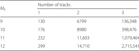
Suppose thatt,max = 3. In Table3, the numbers of joint events for different Mk and different numbers of
tracks are shown. In this table, the number of joint events exponentially grows with the number of tracks and the
number of the path-assigned measurements. t,max is a
parameter predetermined by the designer, and it also has an influence on the number of the joint events.
B. Complexity of the track structure
In this part, the complexities of the track propagation of a track in MD-JITS and MD-JIPDA are analyzed.
Let Bk denote the number of the path-assigned
measurement cells represented by zt,nt(k)|M t jk
zt,nt(k) including the special case 0|0. In MD-JITS, each measurement cell and path model combination (zt,nt(k)|M
t jk
zt,nt(k)
or 0|0) is combined to
the parent componentκt,k−1to make a new component. Thus, component κt,k−1 becomes B
k new components
after processing the combinations. Finally, the total
num-ber of new components becomesK·Bk after processing
all the combinations with all theK parent components. For each component, as well as for each track, the state estimate and the a posteriori component probability are computed recursively. The MD-JITS track propagation has the complexity ofO(K·Bk)at scank. The
complex-ity of this algorithm increases as the increasing of the number of measurement.
The number of components grows exponentially in time. Practical implementation of MD-JITS must include procedures to control the number of components. Com-ponent merging and pruning techniques have been described in [37].
Each track in MD-JIPDA keeps only one Gaussian pdf, representing the track state estimate. At scank,Bk
combi-nations are associated to a track. This association problem can be solved with the complexityO(Bk).
4 Results and discussion
In this section, the simulation performances of MD-JIPDA and MD-JITS are compared. In total, 250 Monte Carlo simulation runs are employed, where each run com-prises 40 scans. Four targets exist from the initial scan to
Table 3Number of joint events
Mk
Number of tracks
1 2 3
9 130 6799 136,348
10 176 8980 398,476
11 232 11,603 1,079,464
12 299 14,710 2,715,541
the final scan, and they propagate according to a nearly constant velocity (NCV) model. In each of the simulation runs, the influence of process noise is added to the true target trajectories, as shown in Fig.2. Target 1 and target 2 intersect at scan 30. Both MD-JIPDA and MD-JITS use the same measurement set for the simulations.
The OTHR system geometry is as shown in Fig. 1,
and the information on the surveillance area is given in Table4. The average number of the clutter measurements at each scan is set to be 25. The NCV model for target dynamics is employed as
x(k)=Fx(k−1)+v(k−1), (33)
wherex(k)is the target state at scank, the sampling inter-val is 20 s,Fis the state propagation matrix, andv(k−1) is the zero-mean Gaussian process noise with covariance Q. The process noise covariance is given by
Q=blockdiag
&
7.8×10⁻¹, 4.4×10⁻⁴ 4.4×10⁻⁴, 1.3×10⁻⁵
'
,
&
1.5×10⁻¹², 1.1×10⁻¹³ 1.1×10⁻¹³, 1.1×10⁻¹⁴
'
,
(34)
The target measurementRg,Rr,Az
in(km, km/s, rad) is generated by (3) including the zero-mean Gaussian
measurement noise with covarianceRgiven by
R=diag25km2, 1×10⁻⁶km2/s2, 9×10⁻⁶rad2. (35)
The target state contains information on the range, range rate, bearing, and bearing ratex(k)=ρ ρ˙ b b˙T, and the initial target states are given in Table5. The tar-get detection probability of each pathPDand the gating
probabilityPGare given in Table5.
The initial track state covariance, which is needed in the track initialization step, is given by
P0|0=diag25km2, 1×10⁻⁵km2/s2, 9×10⁻⁶rad2, 6.4×10⁻⁸rad2/s2.
(36)
The rate of bearing is set to be 0 in the initialization step. Some of those parameters are the same as given in [39]. The transitional probabilities used in the Markov chain process are given by
&
P11 P21 P12 P22
'
=
&
0.98 0 0.02 1
'
(37)
1000 1050 1100 1150 1200 1250 1300 1350 1400
Range (km)
0.08 0.1 0.12 0.14 0.16 0.18 0.2
Bearing (rad) Target 1
Target 1 Start Point Target 2 Target 2 Start Point Target 3 Target 3 Start Point Target 4 Target 4 Start Point
Fig. 2True target trajectories
⎧ ⎪ ⎪ ⎨ ⎪ ⎪ ⎩
ρ=2
r12−h2 r ˙
ρ=4Rr/r1+(η/r2)(ρ/r1+η/r2) b=sin−1
sin(Az) cos(ϕ)
,
(38)
where
0
r1= R 2
g+h2r−h2t−(d/ 2)2
2Rg−dsin(Az) r2=Rg−r1.
(39)
4.1 False track discrimination and track accuracy
The tracking performance is tested with emphasis on the false track discrimination and tracking accuracy. Both MD-JIPDA and MD-JITS use the probability of target existence to solve the false track discrimination issue as follows:
• A track is initialized by the one-point initialization method. Each track is assigned an initial probability of target existence in the track initialization step. The values of the initial probability of target existence for
Table 4Surveillance area parameters
Parameter Value
Slant range size 1000–1400 km
Rate of slant range size 0.013889–0.22222 km/s
Apparent azimuth size 0.069813–0.17453 rad
T to R distanced 100 km
Hight of layerE 100 km
Hight of layerF 260 km
MD-JIPDA tracks and MD-JITS tracks are different, ensuring that those two trackers have the same number of confirmed false tracks.
• The probability of target existence of a track is updated scan by scan, and once it exceeds the confirmation probability of target existence (0.98), the track becomes a confirmed track.
• The confirmed track is tested as to whether it is a confirmed true track or a confirmed false track by the following criteria:
(x˜(k|k))TP0−|10x˜(k|k) <20for comfirmed true track,
(x˜(k|k))TP0−|10x˜(k|k) >40for comfirmed false track. (40)
Here,x˜(k|k)=x(k)− ˆx(k|k)is the state estimation error of a confirmed track at timek andP0|0is the
initial state covariance given in (32).
• If the probability of target existence of a track is lower than the termination probability of target existence
Table 5Target parameters
Parameter Value
Target1 1050 km; 0.15 km/s; 0.10472 rad; 8.72665×10⁻⁵rad/s
Target2 1225 km;−0.14 km/s; 0.11472 rad; 7.72665×10⁻⁵rad/s
Target3 1300 km; −0.17 km/s; 0.14701 rad;−4.72665×10⁻⁵rad/s
Target4 1050 km; 0.1 km/s; 0.18701 rad; 0 rad/s
PD 0.4
(initial probability of target existence/5), the track is terminated.
The simulation parameters used for JITS and MD-JIPDA are given in Table6. For the fair comparison, the confirmation probabilities of target existence (confirma-tion PTE) of MD-JIPDA and MD-JITS are set to be the same and the initial probabilities of target existence (ini-tial PTE) of these two algorithms are adjusted so that both of these two algorithms obtain the same number of confirmed false tracks (CFT).
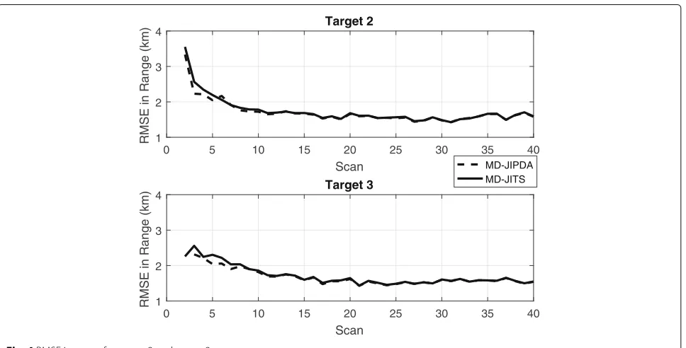
The simulation performances are given as in Fig. 3
through Fig.5. Since the tracking performances for these four targets are very similar, only performances for tar-get 2 and tartar-get 3 are shown in this paper. The numbers of the confirmed true tracks (CTTs) of both algorithms
in 250 Monte Carlo runs are shown in Fig.3 for target
2 and target 3. The numbers of confirmed true tracks of MD-JIPDA and MD-JITS are compared under the condi-tion that both of the two trackers have the same number of confirmed false tracks (=9). These two figures indicate that MD-JITS has a faster confirmation rate for obtain-ing 250 confirmed true tracks (100 percent) compared to MD-JIPDA.
Figure4depicts the RMSEs (root mean square errors)
in the range estimation for target 2 and target 3. In earlier scans, there is a small difference between these two track-ers, while both the trackers eventually maintain the same level of estimation accuracy.
The RMSEs in the bearing of target 2 and target 3 are shown in Fig.5. The RMSEs in the bearing first increase due to the bearing rate being set as 0 in the track ini-tialization step, and so both of these two trackers need some time to recover this parameter. Then, the estima-tion error in the bearing estimaestima-tion is reduced as the number of scans increases. All these simulation results demonstrate the benefits of using MD-JITS. MD-JITS out-performs MD-JIPDA, especially in terms of false track discrimination, while MD-JITS maintains the same esti-mation accuracy in terms of RMSE in both range and bearing estimates.
This simulation is implemented on a 4.00 GHz, Intel Core i7 PC and run with MATLAB. The CPU time per each Monte Carlo run for MD-JIPDA and MD-JITS are 345.7360 s and 349.3160 s, respectively. The simulation
Table 6Tracker parameters
MD-JIPDA MD-JITS
Initial PTE 0.000001 0.0017
Confirmation PTE 0.98 0.98
Termination PTE 0.000001/5 0.0017/5
Number of CFT 9 9
time is similar since most of the computational load is assigned to the joint measurements-to-track assignment part, which is identical for both MD-JIPDA and MD-JITS. Since MD-JITS needs to maintain track components, the computational cost of MD-JITS is a little bit higher than that of MD-JIPDA.
All the simulation results suggest that MD-JITS has bet-ter true track confirmation performances compared to MD-JIPDA. However, in order to achieve this benefit, MD-JITS is more time-consuming.
4.2 A measure for the multi-path track discrimination In the OTHR system, there is a special kind of tracks called the multi-path track [39]. The multi-path track is generated due to an incorrect combination between the measurements and the propagation models at each scan. The multi-path track is different from the false track since the multi-path track uses target measurement to update the track state and propagate parallel to the true target tra-jectory, while the false track is updated by using the clutter measurement and wanders away from the true target tra-jectory. Thus, one of the tasks when using the OTHR tracking system is to distinguish between the multi-path track and the true track. The mechanism analysis details are given in [26]. Following this, we propose a method for both MD-JIPDA and MD-JITS to distinguish the multi-path tracks.
The maximum number of measurement paths (models) for each target is defined asL. Here, we define a variable vector atk,1,akt,2,. . .,atk,L (atk,i ∈ {0, 1},i = 1, 2,. . .L) that is used to count the active paths at scankfor trackt. atk,i =1 means that pathiis active at scank, andatk,i =0 means that pathiis not active at scank. In MD-JIPDA, the state estimation is generated by a Gaussian mixture considering all of the data association events, where each event represents the track state pdf for the track involved in the event. Among all the data association events of a track, the one with the highest data association probability is selected and the measurement path models considered in this data association event are counted. For example, in the event that has the highest data association probability, it turns out thatz1(k) andz3(k) are considered as tar-get detections.z1(k)comes from path 1 andz3(k)comes from path 2; thus, the corresponding active model vector is
atk,1,atk,2,atk,3,atk,4
0 5 10 15 20 25 30 35 40
Scan
0 50 100 150 200 250
Number of CTTs
Target 2
MD-JIPDA MD-JITS
0 5 10 15 20 25 30 35 40
Scan
0 50 100 150 200 250
Number of CTTs
Target 3
Fig. 3Number of CTTs for target 2 and target 3
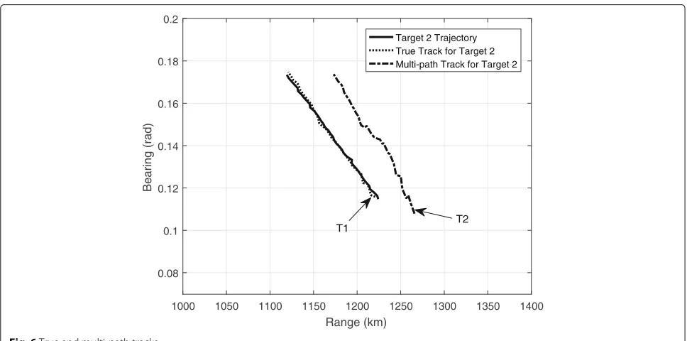
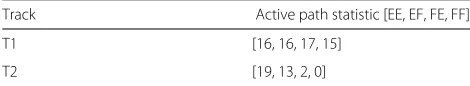
Multi-path tracks exist in this surveillance scenario, and the trajectories for two tracks (one is the true track and another is the multi-path track) for one simulation for MD-JITS are shown in Fig. 6. In this figure, the track T1 represents the true track for target 2 and T2 repre-sents the multi-path track for target 2. In Table 7, the estimated active model calculated by the method intro-duced in this section is listed. From the table, we can
see that the active mode values of the multi-path track are significantly different across the models, which can be used to distinguish the multi-path tracks from the
true tracks. Given that PD = 0.4 for target
measure-ment from each path, the accumulated path statistic of T1 in Table7shows almost 16 detections in 40 scans for
each measurement path. However,T2 does not show this
tendency.
0 5 10 15 20 25 30 35 40
Scan 1
2 3 4
RMSE in Range (km)
Target 2
MD-JIPDA MD-JITS
0 5 10 15 20 25 30 35 40
Scan 1
2 3 4
RMSE in Range (km)
Target 3
0 5 10 15 20 25 30 35 40
Scan
0.5 1 1.5 2 2.5
RMSE in Bearing (rad)
10-3 Target 2
MD-JIPDA MD-JITS
0 5 10 15 20 25 30 35 40
Scan
0.5 1 1.5 2 2.5
RMSE in Bearing (rad)
10-3 Target 3
Fig. 5RMSE in bearing for target 2 and target 3
5 Conclusions
In this paper, in order to jointly resolve the measure-ment origin uncertainty and measuremeasure-ment path model uncertainty in the OTHR system, we developed the MD-JITS filter. The main benefit of this approach is that it generates all possible target-oriented measurement combinations with validated measurements considering
possible measurement propagation models. The tar-get state information contained in measurements are more efficiently extracted due to one-to-many, track-to-measurement cell association for this multiple detection problem instead of the existing one-to-one associa-tion for single detecassocia-tion. Compared to the widely used PDA framework, MD-JITS is a multi-scan tracker that
1000 1050 1100 1150 1200 1250 1300 1350 1400
Range (km)
0.08 0.1 0.12 0.14 0.16 0.18 0.2
Bearing (rad)
Target 2 Trajectory True Track for Target 2 Multi-path Track for Target 2
T1 T2
Table 7Active model statistic
Track Active path statistic [EE, EF, FE, FF]
T1 [16, 16, 17, 15]
T2 [19, 13, 2, 0]
maintains information on the measurement cell history and propagates based on the components, making it more robust in harsh tracking environments.
To demonstrate the superiority of the proposed MD-JITS filter, we compared it with the MD-JIPDA filter in a MTT environment using the OTHR system. The simu-lation results indicate that the new filter outperforms the MD-JIPDA filter for true track confirmation and mainte-nance and shows the same state estimation accuracy as the MD-JIPDA filter.
There are several aspects worthy for the further work: the method which considers the time varying heights of the ionospheric layers can be inserted into the MD-JITS structure; the more computationally efficient structure of the MD-JITS algorithm is expected to be developed.
Acknowledgements
The authors would like to thank the anonymous reviewers for the improvement of this paper.
Funding
This work was supported by Hanwha Systems, Radar R&D Center through Grant U-17-017.
Availability of data and materials
The datasets supporting the conclusions of this article are included within the article (and its additional file(s)).
Authors’ contributions
YH made the main contributions to conception and tracking algorithms’ design, as well as drafting the article. TLS offered critical suggestions on the algorithms’ design, provided significant revising for important intellectual content, and gave final approval of the current version to be submitted. JHL helped to answer the reviewers’ questions and revise the manuscript. All the authors read and approved the final manuscript.
Authors’ information
YH was born in Hubei, China, in 1990. He received the B.Sc. degree in mechanical engineering and automation from Wuhan University of Science and Technology, Wuhan, China, in 2013. He is currently working toward a Ph.D. degree in Hanyang University. His research interests include target state estimation and information fusion.
TLS was born in Andong, Korea, in 1952. He received the B.Sc. degree in nuclear engineering from Seoul National University, Seoul, Korea, in 1974, and both the M.Sc. and Ph.D. degrees in aerospace engineering from the University of Texas at Austin, in 1981 and 1983, respectively. From 1974 to 1994, he was with the Agency for Defense Development where his major research topics included missile guidance and control and control systems design, target tracking, and navigation systems analysis. He has been a Professor at the Electronic Systems Engineering Department, Hanyang University, since 1995. His research interests include target state estimation, guidance, navigation, and control. JHL was born in Seoul, Korea, in 1980. He received the B.Sc. degree in computer engineering and an M.Sc. degree in control engineering from Hanyang University in 2006 and 2008, respectively. He is currently working as a senior engineer at Radar R&D Center of Hanwha Systems.
Competing interests
The authors declare that they have no competing interests.
Publisher’s Note
Springer Nature remains neutral with regard to jurisdictional claims in published maps and institutional affiliations.
Author details
1Department of Electronic Systems Engineering, Hanyang University,
Hanyangdaehak-ro, Ansan, Republic of Korea.2Radar R&D Center, Hanwha
Systems, GyeonggiDong-ro, Yongin, Republic of Korea.
Received: 2 January 2018 Accepted: 4 September 2018
References
1. Y. Bar-Shalom, X. R. Li, T. Kirubarajan,Estimation with application to tracking and navigation. (Wiley Press, New York, 2001)
2. S. Challa, R. Evans, M. Morelande, D. Musicki,Fundamentals of object tracking. (Cambridge University, United Kingdom, 2011)
3. Y. Bar-Shalom, P. Willett, X. Tian,Tracking and data fusion: a handbook of algorithms. (YBS, Bloomfield, 2011)
4. D. Musicki, R. Evans, S. Stankovic, Integrated probabilistic data association (IPDA). IEEE Trans. Automat. Contr.39(6), 1237–1241 (1994)
5. D. B. Reid, H. Thomas, An algorithm for tracking multiple targets. IEEE Trans. Automat. Contr.24(6), 843–854 (1979)
6. Y. Bar-Shalom, E. Tse, Tracking in a cluttered environment with probabilistic. Automatica.11(5), 451–460 (1975)
7. R. Mahler, Aerosp, Multitarget Bayes filtering via first-order multitarget moments. IEEE Trans. Electron. Syst.39(4), 1152–1178 (2003) 8. S. Reuter, B. T. Vo, B. N. Vo, The labeled multi-Bernoulli filter. IEEE Trans.
Signal Process.62(12), 3245–3260 (2014)
9. A. M. Aziz, A joint possibilistic data association technique for tracking multiple targets in a cluttered environment. Inform. Sciences.280(1), 239–260 (2014)
10. H. Zhu, H. Leung, K. V. Yuen, A joint data association, registration, and fusion approach for distributed tracking. Inform. Sciences.324(10), 186–196 (2015)
11. D. Musicki, R. Evans, Multiscan multitarget tracking in clutter with integrated track splitting filter. IEEE Trans. Aerosp. Electron. Syst.45(4), 1432–1447 (2009)
12. T. Kurien,Multitarget multisensor tracking: advanced applications. (Artech House, Norwood, 1990)
13. D. Avitzour, A maximum likelihood approach to data association. IEEE Trans. Aerosp. Electron. Syst.28(2), 560–566 (1996)
14. D. Ciuonzo, S. Horn, A hash-tree based approach for a totally distributed track oriented multi hypothesis tracker. Proc. Int. Conf. IEEE Aerosp, 1–9 (2012)
15. D. Musicki, R. Evans. IEEE Trans. Aerosp. Electron. Syst.40(3), 1093–1099 (2004)
16. D. Ciuonzo, P. K. Willett, Y. Bar-Shalom, Tracking the tracker from its passive sonar ML-PDA estimates. IEEE Trans. Aerosp. Electron. Syst.50(1), 573–590 (2014)
17. Y. F. Guo, R. Tharmarasa, S. Rajan, T. L. Song, T. Kirubarajan, Passive tracking in heavy clutter with sensor location uncertainty. IEEE Trans. Aerosp. Electron. Syst.52(4), 1536–1554 (2016)
18. S. Blackman,Multiple-target tracking with radar applications. (Artech House, Norwood, 1986)
19. D. J. Salmond, Mixture reduction algorithms for target tracking in clutter. Proc. Int. Conf. Signal Data Process Small Targets.1305, 434–445 (1990) 20. D. Musicki, B. L. Scala, R. Evans, Integrated track splitting filter efficient
multi-scan single target tracking in clutter. IEEE Trans. Aerosp. Electron. Syst.43(4), 1409–1425 (2007)
21. T. H. Kim, T. L. Song, Multi-target multi-scan smoothing in clutter. IET Radar Sonar. Navig.10(7), 1270–1276 (2016)
22. W. G. Pulford, R. Evans, A multipath data association tracker for over-the-horizon radar. IEEE Trans. Aerosp. Electron. Syst.34(4), 1165–1183 (1998)
23. W. G. Pulford, R. Evans, Authors’ reply to ‘comments on “multipath data association tracker for over-the-horizon rada”’. IEEE Trans. Aerosp. Electron. Syst.41(3), 1148–1150 (1998)
25. T. Sathyan, T. J. Chin, S. Arulampalam, D. Suter, A multiple hypothesis tracker for multitarget tracking with multiple simultaneous measurements. IEEE J-STSP.7(3), 448–460 (2013)
26. J. F. Chen, H. Ma, C. G. Liang, OTHR multipath tracking using the Bernoulli filter. IEEE Trans. Aerosp. Electron. Syst.50(3), 1974–1990 (2014) 27. X. Tang, X. Chen, M. McDonald, R. Mahler, R. Tharmarasa, T. Kirubarajan, A
multiple-detection probability hypothesis density filter. IEEE Trans. Signal Process.63(8), 2007–2019 (2015)
28. Y. Qin, H. Ma, L. Cheng, L. Yang, X. Q. Zhou, Cardinality balanced multitarget multi-Bernoulli filter for multipath multitarget tracking in over-the-horizon radar. IET Radar Sonar Navig.10(3), 535–545 (2016) 29. Y. Qin, H. Ma, J. F. Chen, L. Cheng, Gaussian mixture probability hypothesis
density filter for multipath multitarget tracking in over-the-horizon radar. EURASIP J. Adv. Signal Process.2015, 108 (2015)
30. D. Nikolio, Z. Popovic, M. Borenovio, N. Stojkovio, V. Orlic, A. Dzvonkovskaya, B. M. Todorovic, Multi-radar multi-target tracking algorithm for maritime surveillance at OTH distances. Proc. Int. Radar Symp. (IRS)., 1–6 (2016)
31. B. Habtemariam, R. Tharmarasa, T. Thayaparan, M. Mallick, T. Kirubarajan, A multiple-detection joint probabilistic data association filter. IEEE J. Sel. Top. Signal Process.7(3), 461–471 (2013)
32. Y. Huang, T. L. Song, C. M. Lee, The multiple detection joint integrated track splitting filter. Proc. CIE Int. Conf. Radar, 1–4 (2016)
33. M. Kong, G. H. Wang, J. Bai, Research on target tracking technology of OTHR based on MPDA. Proc. Int. Conf. Radar, 1–4 (2006)
34. H. Geng, Y. Liang, F. Yang, L. F. Xu, Joint estimation of target state and ionosphere state for OTHR based tracking. Proc. Int. Conf. Inf. Fusion, 1270–1277 (2015)
35. H. Geng, Y. Liang, F. Yang, L. F. Xu, Q. Pan, Joint estimation of target state and ionospheric height bias in over-the-horizon radar target tracking. IET Radar Sonar. Navig.10(7), 1153–1167 (2016)
36. H. Geng, Y. Liang, X. X. Wang, F. Yang, L. F. Xu, Q. Pan, Multi-path multi-rate filter for OTHR based tracking systems. Proc. Int. Conf. Inf. Fusion, 1276–1283 (2016)
37. S. Blackman, R. Popoli,Design and analysis of modern tracking systems. (Artech House, Boston, 1999)
38. F. W. Smith, J. A. Malin, Models for radar scatterer density in terrain images. IEEE Trans. Aerosp. Electron. Syst.AES-22(5), 642–647 (1986) 39. H. Lan, Y. Liang, Q. Pan, An EM algorithm for multipath state estimation in