Research-An Introduction: Report 1 of the ISPOR Optimization Methods Emerging Good
Practices Task Force..
White Rose Research Online URL for this paper:
http://eprints.whiterose.ac.uk/114058/
Version: Accepted Version
Article:
Crown, W., Buyukkaramikli, N., Thokala, P. et al. (8 more authors) (2017) Constrained
Optimization Methods in Health Services Research-An Introduction: Report 1 of the
ISPOR Optimization Methods Emerging Good Practices Task Force. Value Health, 20 (3).
pp. 310-319. ISSN 1098-3015
https://doi.org/10.1016/j.jval.2017.01.013
Article available under the terms of the CC-BY-NC-ND licence
(https://creativecommons.org/licenses/by-nc-nd/4.0/)
[email protected] https://eprints.whiterose.ac.uk/ Reuse
This article is distributed under the terms of the Creative Commons Attribution-NonCommercial-NoDerivs (CC BY-NC-ND) licence. This licence only allows you to download this work and share it with others as long as you credit the authors, but you can’t change the article in any way or use it commercially. More
information and the full terms of the licence here: https://creativecommons.org/licenses/
Takedown
If you consider content in White Rose Research Online to be in breach of UK law, please notify us by
1
Constrained Optimization Methods in Health Services Research – An Introduction: Report 1 of the ISPOR Optimization Methods Emerging Good Practices Task Force
William Crown, PhD1,*, Nasuh Buyukkaramikli, PhD2, Praveen Thokala, PhD3, Alec Morton, PhD4, Mustafa Y. Sir, PhD5, Deborah A. Marshall, PhD6, Jon Tosh, PhD7, William
V. Padula, PhD, MS8, Maarten J. Ijzerman, PhD9, Peter K. Wong, PhD, MS, MBA, RPh10, Kalyan S. Pasupathy, PhD11,*
1 Optum Labs, Boston, MA, USA; 2 Scientific Researcher, institute of Medical Technology assessment,
1Erasmus University Rotterdam, Rotterdam, The Netherlands; 3 Research Fellow, University of Sheffield,
2Sheffield, UK; 4 Professor of Management Science, Department of Management Science, Strathclyde
3Business School, University of Strathclyde, Glasgow, Scotland, UK; 5 Assistant Professor, Health Care
4Policy & Research, Faculty - Information and Decision Engineering, Mayo Clinic Robert D. and Patricia
5E. Kern Center for the Science of Health Care Delivery, Rochester, MN, USA; 6 Canada Research Chair,
6Health Services & Systems Research; Arthur J.E. Child Chair in Rheumatology Research; Director, HTA,
7Alberta Bone & Joint Health Institute; Associate Professor, Department Community Health Sciences,
8Faculty of Sciences, Faculty of Medicine, University of Calgary, Calgary, Alberta, Canada; 7 Senior
9Health Economist, DRG Abacus, Manchester, UK; 8 Assistant Professor, Department of Health Policy &
10Management, Johns Hopkins Bloomberg School of Public Health, Baltimore, MD, USA; 9 Professor of
11Clinical Epidemiology & Health Technology Assessment (HTA); Head, Department of Health Technology
12& Services Research, University of Twente, Enschede, The Netherlands; 10 Vice President and Chief
13Performance Improvement Officer, Illinois Divisions and HSHS Medical Group, Hospital Sisters Health
14System (HSHS), Belleville, IL. USA; 11 Associate Professor - Healthcare Policy & Research, Scientific
15Director
–
Clinical Engineering Learning Labs, Lead
–
Information and Decision Engineering, Mayo
16Clinic Robert D. and Patricia E. Kern Center for the Science of Health Care Delivery, Rochester, MN,
17USA.
18*Corresponding authors – Kalyan S. Pasupathy ([email protected]) and William Crown ([email protected])
Abstract 19
Providing health services with the greatest possible value to patients and society given the constraints
20
imposed by patient characteristics, health care system characteristics, budgets, etc. relies heavily on the
21
design of structures and processes. Such problems are complex and require a rigorous and systematic
22
approach to identify the best solution. Constrained optimization is a set of methods designed to identify
23
efficiently and systematically, the best solution (the optimal solution) to a problem characterized by a
24
number of potential solutions in the presence of identified constraints. This report identifies: 1) key
25
concepts and the main steps in building an optimization model; 2) the types of problems where optimal
26
solutions can be determined in real world health applications and 3) the appropriate optimization
27
methods for these problems. We first present a simple graphical model based upon the treatment of
28
2
constraints. We then relate it back to how optimization is relevant in health services research for
30
addressing present day challenges. We also explain how these mathematical optimization methods relate
31
to simulation methods, to standard health economic analysis techniques, and to the emergent fields of
32
analytics and machine learning.
33
Keywords: Decision making, care delivery, policy, modeling
3 1. Introduction
35
In common vernacular, the term “optimal” is often used loosely in health care applications to refer to any
36
demonstrated superiority among a set of alternatives in specific settings. Seldom is this term based on
37
evidence that demonstrates such solutions are, indeed, optimal – in a mathematical sense. By “optimal”
38
solution we mean the best possible solution for a given problem given the complexity of the system inputs,
39
outputs/outcomes, and constraints (budget limits, staffing capacity, etc.). Failing to identify an “optimal”
40
solution represents a missed opportunity to improve clinical outcomes for patients and economic
41
efficiency in the delivery of care.
42 43
Identifying optimal health system and patient care interventions is within the purview of mathematical
44
optimization models. There is a growing recognition of the applicability of constrained optimization
45
methods from operations research to health care problems. In a review of the literature [1], note more
46
than 200 constrained optimization and simulation studies in health care. For example, constrained
47
optimization methods have been applied in problems of capacity management and location selection for
48
both healthcare services and medical supplies [2-5].
49
Constrained optimization is an interdisciplinary subject, cutting across the boundaries of mathematics,
50
computer science, economics and engineering. Analytical foundations for the techniques to solve the
51
constrained optimization problems involving continuous, differentiable functions and equality constraints
52
were already laid in the 18th century [6]. However, with advances in computing technology, constrained 53
optimization methods designed to handle a broader range of problems trace their origin to the
54
development of the simplex algorithm--the most commonly used algorithm to solve linear constrained
55
optimization problems--in 1947 [7-11]. Since that time, a variety of constrained optimization methods
56
have been developed in the field of operations research and applied across a wide range of industries. This
57
creates significant opportunities for the optimization of health care delivery systems and for providing
58
value by transferring knowledge from fields outside the health care sector.
59
In addition to capacity management, facility location, and efficient delivery of supplies, patient scheduling,
60
provider resource scheduling, and logistics are other substantial areas of research in the application of
61
constrained optimization methods to healthcare [12-16]. Constrained optimization methods may also be
62
very useful in guiding clinical decision-making in actual clinical practice where physicians and
63
patients face constraints such as proximity to treatment centers, health insurance benefit designs,
64
and the limited availability of health resources.
65
Constrained optimization methods can also be used by health care systems to identify the optimal
66
allocation of resources across interventions subject to various types of constraints [17-23]. These methods
67
have also been applied to disease diagnosis [24, 25], the development of optimal treatment algorithms
68
[26, 27], and the optimal design of clinical trials [28]. Health technology assessment using tools from
69
constrained optimization methods is also gaining popularity in health economics and outcomes research
70
[29].
71
Recently, the ISPOR Emerging Good Practices Task Force on Dynamic Simulation Modeling Applications
72
in Health Care Delivery Research published two reports in Value in Health [30, 31] and one in
73
Pharmacoeconomics [32] on the application of dynamic simulation modeling (DSM) to evaluate problems
74
in health care systems. While simulation can provide a mechanism to evaluate various scenarios, by
75
design, they do not provide optimal solutions. The overall objective of the ISPOR Emerging Good
76
Practices Task Force on Constrained Optimization Methods is to develop guidance for health services
77
researchers, knowledge users and decision makers in the use of operations research methods to optimize
78
healthcare delivery and value in the presence of constraints. Specifically, this task force will (1) introduce
79
constrained optimization methods for conducting research on health care systems and individual-level
80
outcomes (both clinical and economic); (2) describe problems for which constrained optimization
4
methods are appropriate; and (3) identify good practices for designing, populating, analyzing, testing and
82
reporting results from constrained optimization models.
83
The ISPOR Emerging Good Practices Task Force on Constrained Optimization Methods will produce two
84
reports. In this first report, we introduce readers to constrained optimization methods. We present
85
definitions of important concepts and terminology, and provide examples of health care decisions where
86
constrained optimization methods are already being applied. We also describe the relationship of
87
constrained optimization methods to health economic modeling and simulation methods. The second
88
report will present a series of case studies illustrating the application of these methods including model
89
building, validation, and use.
90
2. Definition of Constrained Optimization 91
92
Constrained optimization is a set of methods designed to efficiently and systematically find the best
93
solution to a problem characterized by a number of potential solutions in the presence of identified
94
constraints. It entails maximizing or minimizing an objective function that represents a quantifiable
95
measure of interest to the decision maker, subject to constraints that restrict the decision maker’s freedom
96
of action. Maximizing/minimizing the objective function is carried out by systematically selecting input
97
values for the decision from an allowed set and computing the objective function, in an iterative manner,
98
until the decision yields the best value for the objective function, a.k.a optimum. The decision that gives
99
the optimum is called the “optimal solution”. In some optimization problems, two or more different 100
decisions may yield the same optimum. Note that, programming and optimization are often used as
101
interchangeable terms in the literature, e.g., linear programming and linear optimization. Historically,
102
programming referred to the mathematical description of a plan/schedule, and optimization referred to
103
the process used to achieve the optimal solution described in the program.
104 105
The components of a constrained optimization problem are its objective function(s), its decision
106
variable(s) and its constraint(s). The objective function is a function of the decision variables that
107
represents the quantitative measure that the decision maker aims to minimize/maximize. Decision 108
variables are mathematical representation of the constituents of the system for which decisions are being
109
taken to improve the value of the objective function. The constraints are the restrictions on decision
110
variables, often pertaining to resources. These restrictions are defined by equalities/inequalities involving
111
functions of decision variables. They determine the allowable/feasible values for the decision variables. In
112
addition, parameters are constant values used in objective function and constraints, like the multipliers
113
for the decision variables or bounds in constraints. Each parameter represents an aspect of the
decision-114
making context: for example, a multiplier may refer to the cost of a treatment.
115
3. A Simple Illustration of a Constrained Optimization Problem 116
117
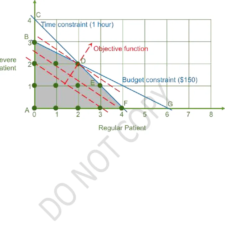
Imagine you are the manager of a health care center, and your aim is to benefit as many patients as
118
possible. Let us say, for the sake of simplicity, you have two types of patients-- regular and severe patients,
119
and the demand for the health service is unlimited for both of these types. Regular patients can achieve
120
two units of health benefits and severe ones can achieve three units. Each patient, irrespective of severity,
121
takes 15 minutes for consultation; only one patient can be seen at any given point in time. You have one
122
hour of total time at your disposal. Regular patients require $25 of medications, and severe patients
123
require $50 of medications. You have a total budget of $150. What is the greatest health benefit this
124
center can achieve given these inputs and constraints?
125
At the outset, this problem seems straightforward. One might decide on four regular patients to use up all
126
the time that is available. This will achieve eight units of health benefit while leaving $50 as excess budget.
127
An alternate approach might be to see as many severe patients as possible since treating each severe
128
patient generates more per capita health benefits. Three patients (totaling $150) would generate 9 health
5
units leaving 15 minutes extra time unused. There are other combinations of regular and severe patients
130
that would generate different levels of health benefits and use resources differently.
131
This is graphically represented in Figure 1, with regular patients on the x-axis and the severe patients on
132
the y-axis. Line CF is the time constraint limiting total time to one hour. Line BG is the budget constraint
133
limiting to $150. Any point to the south-west of these constraints (lines) respectively, will ensure that time
134
and budget do not exceed the respective limits. The combination of these together with non-negativity of
135
the decision variables, gives the feasible region.
136
The lines AB-BD-DF-FA form the boundary of the feasibility space, shown shaded in the figure. In
137
problems that are three or more dimensional, these lines would be hyperplanes. To obtain the optimal
138
solution, the dashed line is established, the slope depends on the relative health units of the two decision
139
variables (i.e., the number of regular and severe patients seen). This dashed line moves from the origin in
140
the north-east direction as shown by the arrow. The optimal solution is two regular patients and two
141
severe patients. This approach uses the entire one-hour time as well as the $150 budget. Since regular and
142
severe patients achieve two- and three-unit health benefits, respectively, we are able to achieve 10 units of
143
health benefit and still meet the time and budget constraints.
144
No other combination of patients is capable of achieving more benefits while still meeting the time and
145
budget constraints. Note that not all resource constraints have to be completely used to attain the optimal
146
solution. This hypothetical example is a small-scale problem with only two decision variables; the number
147
of regular and severe patients seen. Hence, they can be represented graphically with one variable on each
148
axis.
149
With the difficulty in representing larger problems graphically, we turn to mathematical approaches, such
150
as the simplex algorithm to find the solutions. The simplex algorithm is a structured approach of
151
navigating the boundary (represented as lines in two dimensions and hyperplanes in three or more
152
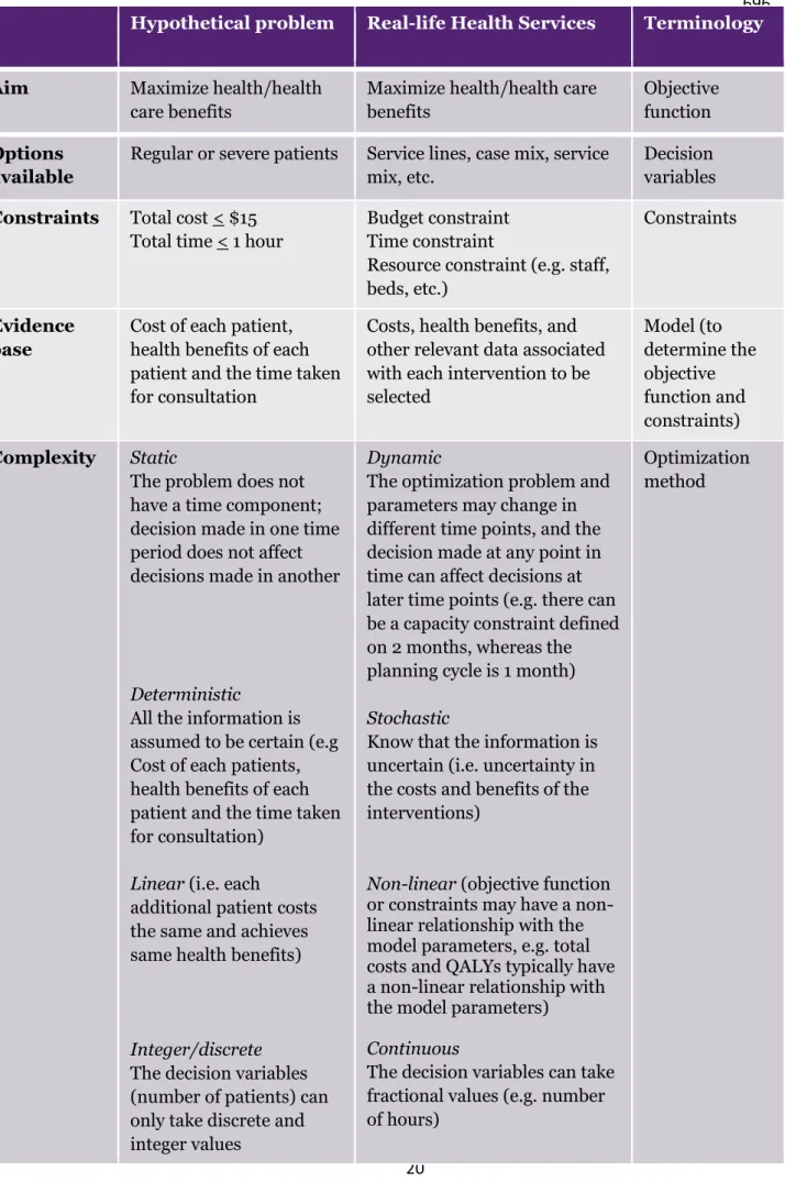
dimensions) of the feasibility space to arrive at the optimal solution. Table 1 summarizes the main
153
components of the example and notes several other dimensions of complexity (linear vs nonlinear,
154
deterministic vs stochastic, static vs dynamic, discrete/integer vs continuous) that can be incorporated
155
into constrained optimization models.
156
6
Figure 1. Graphical Representation of Solving a Simple Integer Programming Problem 158
159
The mathematical formulation of the model is as follows:
160 161
Max fR xR + fL xL (objective function) 162
subject to cR xR + cL xL ≤ B (budget constraint) 163
tR xR + tL xL ≤ T (time constraint) 164
xR ,xL ≥ 0 and integer (decision variables) 165
166
Where:
167
cR,cL= cost of regular and severe patients, respectively 168
B = total budget available
169
tR,tL= time to see regular and severe patients, respectively 170
T = total time available
171
fR,fL= health benefits of regular and severe patients, respectively 172
xR,xL= number of regular and severe patients, respectively 173
174
In the current version of the problem, the parameters are:
175
fR = 2 health benefit units, fL = 3 health benefit units 176
cR = $25, cL = $50, B = $150 177
tR =0.25 hours, tL = 0.25 hours, T = 1 hour 178
179
So the model is as follows:
180 181
Max 2xR + 3xL (objective function) 182
subject to 25xR + 50xL ≤ 150 (budget constraint) 183
0.25xR + 0.25xL ≤ 1 (time constraint) 184
xR ,xL ≥ 0 and integer 185
186
As described above, Figure 1 illustrates the graphical solution to this model. However, problems with
187
higher dimensionality must use mathematical algorithms to identify the optimal solution. The problem
188
described above falls into the category of linear optimization, because although the constraints and the
189
objective function are linear from an algebraic standpoint, the decision variables must be in the form of
190
integers. As it will be discussed further in section 5, there are other optimization modelling frameworks,
191
such as combinatorial, nonlinear, stochastic and dynamic optimization.
192
As the algorithms for integer optimization problems can take much longer to solve computationally than
193
those for linear optimization problems, one alternative is to set the integer optimization problem up and
194
solve it as a linear one. If fractional values are obtained, the nearest feasible integers can be used as the
195
final solution. This should be done with caution, however. First, rounding the solution to the nearest
196
integers can result in an infeasible solution or, and second, even if the rounded solution is feasible, it may
197
not be the optimal solution to the original integer optimization problem. Nonlinear optimization is
198
suitable when the constraints or the objective function are non-linear. In problems, where there is
199
uncertainty, such as the estimated health benefit of each patient might receive in the above example,
200
stochastic optimization techniques can be used.
201
Dynamic optimization (known commonly as dynamic programming) formulation might be useful when
202
the optimization problem is not static, that the problem context and parameters change in time and there
203
is an interdependency among the decisions at different time periods (for instance, when decisions made at
204
a given time interval, say number of patients to be seen now, affects the decisions for other time periods,
7
such as the number of patients to be seen tomorrow). Table 1 summarizes the model components in the
206
hypothetical problem, relates it to health services with examples and identifies the specific terminology.
207
Table 1. Model Summary and Extensions 208
209
4. Problems That Can Be Tackled with Constrained OptimizationApproaches
210 211
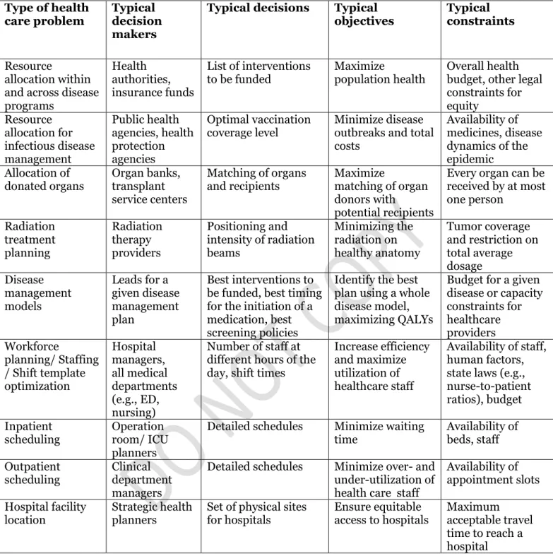
In this section, we list several areas within health care where constrained optimization methods have been
212
used in health services. The selected examples do not represent a comprehensive picture of this field, but
213
provide the reader a sense of what is possible. In Table 2, we compare problems using the terminology of
214
the previous section, with respect to decision makers, decisions, objectives, and constraints.
215
Table 2. Examples of Health Care Decisions for which Constrained Optimization is 216
Applicable 217
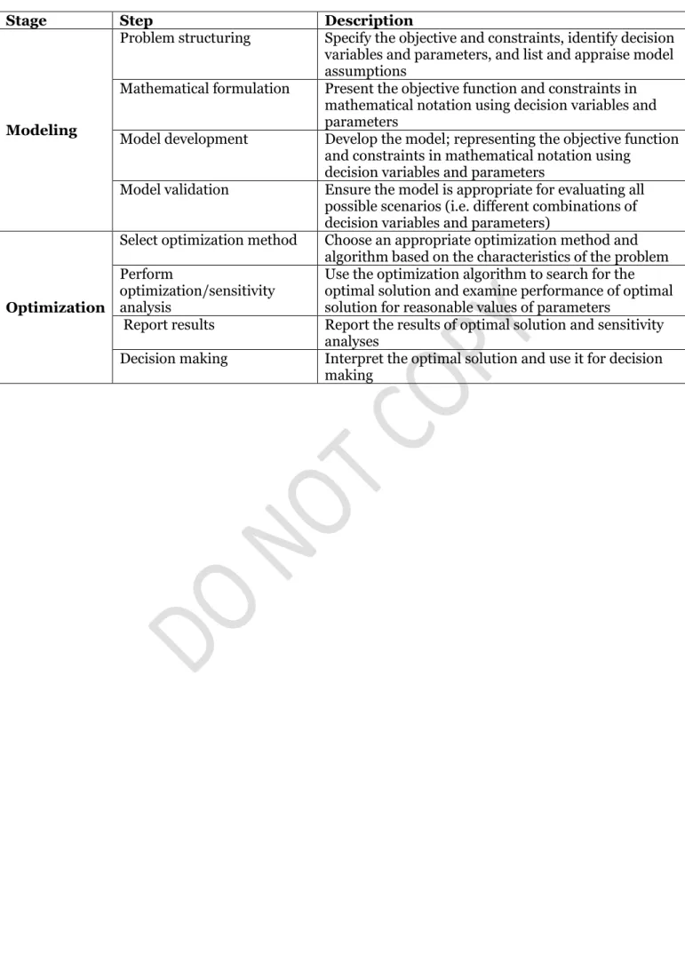
5. Steps in a Constrained Optimization Process 218
219
An overview of the main steps involved in a constrained optimization process [33] is described here and
220
presented in Table 3. Some of the steps are common to other types of modeling methods. It is important to
221
emphasize that the process of optimization is iterative, rather than comprising a strictly sequential set of
222
steps.
223
a) Problem structuring 224
225
This involves specifying the objective, i.e. goal, and identifying the decision variables, parameters and the
226
constraints involved. These can be specified using words, ideally in non-technical language so that the
227
optimization problem is easily understood. This step needs to be performed in collaboration with all the
228
relevant stakeholders, including decision makers, to ensure all aspects of the optimization problem are
229
captured. As with any modeling technique, it is also crucial to surface key modeling assumptions and
230
appraise them for plausibility and materiality.
231
b) Mathematical formulation 232
233
After the optimization problem is specified in words, it needs to be converted into mathematical notation.
234
The standard mathematical notation for any optimization problem involves specifying the objective
235
function and constraint(s) using decision variables and parameters. This also involves specifying whether
236
the goal is to maximize or minimize the objective function. The standard notation for any optimization
237
problem, assuming the goal is to maximize the objective, is as shown below:
238
Maximize z=f(x1, x2, …. xn, p1, p2, …. pk) 239
subject to
240
cj(x1, x2, …. xn, p1, p2, …. pk)≤Cj 241
for j=1,2,..m
242
where, x1, x2, …. xn are the decision variables, f(x1, x2, …. xn) is the objective function; and cj(x1, x2, …. xn, p1, 243
p2, …. pk)≤Cj represent the constraints. Note that the constraints can include both inequality and equality 244
constraints and that the objective function and the constraints also include parameters p1, p2, …. pk, which 245
are not varied in the optimization problem. Specification of the optimization problem in this mathematical
246
notation allows clear identification of the type (and number) of decision variables, parameters and the
247
constraints. Describing the model in mathematical form will be useful to support model development.
248
c) Model development 249
8
The next step after mathematical formulation is model development. Model development involves solving
251
the mathematical problem described in the previous step, and often performed iteratively. The model
252
should estimate the objective function and the left hand side (LHS) values of the constraints, using the
253
decision variables and parameters as inputs. The complexity of the model can vary widely. Similar to
254
other types of modeling, the complexity of the model will depend on the outputs required, the level of
255
detail included in the model, whether it is linear or non-linear, stochastic or deterministic, static or
256
dynamic.
257
d) Perform model validation 258
259
As with any modeling, it is important to ensure that the model developed represents reality with an
260
acceptable degree of fidelity [33]. The requirements of model validation for optimization are more
261
stringent than for, for example, simulation models, due to the need for the model to be valid for all
262
possible combinations of the decision variables. Thus, appropriate caution needs to be taken to ensure
263
that the model assumptions are valid and that the model produces sensible results for the different
264
scenarios. At the very least, the validation should involve checking of the face validity (i.e. experts evaluate
265
model structure, data sources, assumptions, and results), and verification or internal validity (i.e. checking
266
accuracy of coding).
267
e) Select optimization method 268
This step involves choosing the appropriate optimization method, which is dependent on the type of
269
optimization problem that is addressed. Optimization problems can be broadly classified, depending
270
upon the nature of the objective functions and the constraints-for example, into linear vs non-linear,
271
deterministic vs stochastic, continuous vs discrete, or single vs multi-objective optimization. For instance,
272
if the objective function and constraints consist of linear functions only, the corresponding problem is a
273
linear optimization problem. Similarly, in deterministic optimization, the parameters used in the
274
optimization problem are fixed while in stochastic optimization, uncertainty is incorporated. Optimization
275
problems can be continuous (i.e. decision variables are allowed to have fractional values) or discrete (for
276
example a hospital ward may be either open or closed; the number of CT scanners which a hospital buys
277
must be a whole number).
278
Most optimization problems have a single objective function, however when optimization problems have
279
multiple conflicting objective functions, they are referred to as multi-objective optimization problems. The
280
optimization method chosen needs to be in line with the type of optimization problem under
281
consideration. Once the optimization problem type is clear (e.g. discrete or nonlinear), a number of texts
282
may be consulted for details on solution methods appropriate for that problem type [33-36].
283
Broadly speaking, optimization methods can be categorized into exact approaches and heuristic
284
approaches. Exact approaches iteratively converge to an optimal solution. Examples of these include
285
simplex methods for linear programming and the Newton method or interior point method for non-linear
286
programming [34, 37]. Heuristic approaches provide approximate solutions to optimization problems
287
when an exact approach is unavailable or is computationally expensive. Examples of these techniques
288
include relaxation approaches, evolutionary algorithms (such as genetic algorithms), simulated annealing,
289
swarm optimization, ant colony optimization, and tabu-search. Besides these two approaches (i.e. exact or
290
heuristic), other methods are also available to tackle large-scale problems as well (e.g. decomposition of
291
the large problems to smaller sub-problems).
292
There are software programs that help with optimization; interested readers are referred to the website of
293
INFORMS (www.informs.org) for a list of optimization software. The users need to specify, and more
294
importantly understand, the parameters used as an input for these optimization algorithms (e.g., the
295
termination criteria such as the level of convergence required or the number of iterations).
9 f) Perform optimization/sensitivity analysis 297
Optimization involves systematically searching the feasible region for values of decision variables and
298
evaluating the objective function, consecutively, to find a combination of decision variables that achieve
299
the maximum or minimum value of the objective function, using specific algorithms. Once the
300
optimization algorithm has finished running, in some cases, the identified solution can be checked to
301
verify that it satisfies the “optimality conditions” (i.e. Karush-Kuhn-Tucker conditions) [38], which are the
302
mathematical conditions that define the optimality. Once the optimality is confirmed, the results need to
303
be interpreted.
304
First, the results should be checked to see if there is actually a feasible solution to the optimization
305
problem, i.e. whether there is a solution that satisfies all the constraints. If not, then the optimization
306
problem needs to be adjusted, (e.g., relaxing some constraints or adding other decision variables) in order
307
to broaden the feasible solution space. If a feasible optimal solution has been found, the results need to be
308
understood – this involves interpretation of the results to check whether the optimal solution, i.e., values
309
of decision variables, constraints and objective function makes sense.
310
It is also good practice to repeat the optimization with different sets of starting decision variables to
311
ensure the optimal solution is the global optimum rather than local optimum. Sometimes, there may be
312
multiple optimal solutions for the same problem (i.e. multiple combinations of decision variables that
313
provide the same optimal value of objective function). For multi-objective optimization problems (i.e.
314
problems with two or more conflicting objectives), Pareto optimal solutions are constructed from which
315
optimal solution can be identified based on the subjective preferences of the decision maker [39, 40].
316
It is good practice to run the optimization problem using different values of parameters, in order to verify
317
the robustness of the optimization results. Sensitivity analysis is an important part of building confidence
318
in an optimization model, addressing the structural and parametric uncertainties in the model by
319
analyzing how the decision variables and optimum value react to changes in the parameters in the
320
constraints and objective function, which ensures that the optimization model and its solution are good
321
representations of the problem at hand.
322
Sometimes a solution may be the mathematically optimal solution to the specified mathematical problem,
323
but may not be practically implementable. For example, the “optimal” set of nurse rosters may be
324
unacceptable to staff as it involves breaking up existing teams, deploying staff with family responsibilities
325
on night shifts, or reducing overtime pay to level where the employment is no longer attractive. Analysts
326
should resist the temptation to spring their optimal solution on unsuspecting stakeholders, expecting
327
grateful acceptance: rather, those affected by the model should be kept in the loop through the modeling
328
process. The optimal solution may come as a surprise: it is important to allow space in the modeling
329
process to explore fully and openly concerns about whether the “optimal” solution is indeed the one the 330
organization should implement.
331
g) Report results 332
333
The final optimal solution, and if applicable, the results of the sensitivity analyses should be reported. This
334
will include the results of the optimum ‘objective function’ achieved and the set of ‘decision variables’ at 335
which the optimal solution is found. Both the numerical values (i.e. the mathematical solution) and the
336
physical interpretation, i.e., the non-technical text describing the meaning of numerical values, should be
337
presented. The optimal solution identified can be contextualized in terms of how much ‘better’ it is
338
compared to the current state. For example, the results can be presented as improvement in benefits such
339
as QALYs or reduction in costs.
340
10
It is often necessary to report the optimization method used and the results of the ‘performance’ of the
342
optimization algorithm, e.g., number of iterations to the solution, computational time, convergence level,
343
etc. This is important as it helps users understand whether a particular algorithm can be used “online” in a
344
responsive fashion, or only when there is significant time available, e.g. in a planning context. Dashboards
345
can be useful to visualize these benefits and communicate the insights gained from the optimal solution
346
and sensitivity analyses.
347 348
h) Decision making 349
350
The final optimal solution and its implications for policy/service reconfiguration should be presented to all
351
the relevant stakeholders. This typically involves a plan for amending the ‘decision variables’, (e.g., shift
352
patterns, screening frequency--see Table 2 for examples of decision variables--to those identified in the
353
optimal solution). Before an optimal solution can be implemented, it will require getting the ‘buy-in’ from
354
the decision makers and all the stakeholders, e.g., frontline staff such as nurses, hospital managers, etc., to
355
ensure that the numerical ‘optimal’ solution found can be operationalized in a ‘real’ clinical setting. It is
356
important to have the involvement of decision makers throughout the whole optimization process to
357
ensure that it does not become a purely numerical exercise, but rather something that is implemented in
358
real life. After the decision is made, data should still be collected to assess the efficiency and demonstrate
359
the benefits of the implementation of the optimal solution.
360 361
If decision makers are not directly involved in model development they may choose not to implement the
362
“optimal” solution as it comes from the model. This is because the model may fail to capture key aspects
363
of the problem (for example, the model may maximize aggregate health benefits but the decision maker
364
may have a specific concern for health benefits for some disadvantaged subgroup). This does not
365
(necessarily) mean that the optimization modeling has not been useful – enabling a decision maker to see
366
how much health benefit must be sacrificed to satisfy her equity objective may prove to be beneficial
367
towards the overall objective. After the decision is made the story does not come to an end: data should
368
continue to be collected to demonstrate the benefits of whatever solution is implemented, as well as
369
guiding future decision making.
370 371
Table 3 presents the two different stages in optimization i.e. the modeling stage and optimization stage,
372
highlighting that model development is necessary before optimization can be performed. The goal of
373
constrained optimization is to identify an optimal solution that maximizes or minimizes a particular
374
objective subject to existing constraints.
375
Table 3. Steps in an Optimization Process 376
377
6. Relationship of Constrained Optimization to Related Fields 378
379
The use of constrained optimization can be classified into two categories. The first category is the use of
380
constrained optimization as a decision-making tool. The simple illustration in section 3 and all the
381
examples in section 4 are considered to fall under this category. The second category is the use of
382
constrained optimization as an auxiliary analysis tool. In this category, optimization is an embedded tool
383
and the results of which are often not the end results of a decision problem, but rather they are used as
384
inputs for other analysis/modeling methods (e.g. optimization used in the multiple criteria decision
385
making; in calibrating the inputs for health economic or dynamic simulation models; in machine learning
386
and other statistical analysis methods like solving regression models or propensity score matching).
387
As a decision-making tool, optimization is complementary to other modeling methods such as health
388
economic modeling, simulation modeling and descriptive, predictive (e.g. machine learning) and
11
prescriptive analytics. Most modeling methods typically only evaluate a few different scenarios and
390
determine a good scenario within the available options. In contrast, the aim of optimization methods is to
391
efficiently identify the best solution overall, given the constraints. In the absence of using optimization
392
methods, a brute force approach, in which all possible options are sequentially evaluated and the best
393
solution is identified among them, might be possible for some problems. However, for most problems, it is
394
too complex and too time consuming to identify and evaluate all possible options. Optimization methods
395
and heuristic approaches might use efficient algorithms to identify the optimal solution quickly, which
396
would otherwise be very difficult and time consuming.
397
Also, model development using these other methods might be necessary before optimization, especially in
398
situations where the objective function or constraints cannot be represented in a simple functional form.
399
Thus, all models currently used in health care such as health economic models, dynamic simulation
400
models and predictive analytics (including machine learning) can be used in conjunction with
401
optimization methods.
402
a) Constrained Optimization Methods Compared with Traditional Health Economic 403
Modeling in Health Technology Assessments 404
405
Constrained optimization methods differ substantially from health economic modeling methods
406
traditionally used in health technology assessment processes [41]. The main difference between the two
407
approaches is that traditional health economic modeling approaches, such as Markov models, are built to
408
estimate the costs and effects of different diagnostic and treatment options. If decision makers are basing
409
their judgements on modeling results, they may not formally consider the constraints and resource
410
implications in the system. Constrained optimization methods provide a structured approach to optimize
411
the decision problem and to present the best alternatives given an optimization criterion, such as
412
constrained budget or availability of resources.
413
These differences have major implications. There is an opportunity to learn from optimization methods to
414
improve Health Technology Assessment (HTA) processes [42-46]. Optimization is a valuable means of
415
capturing the dynamics and complexity of the health system to inform decision making for several
416
reasons. Constrained optimization methods can:
417
i. Explicitly take budget constraints into account - Informed decision making about resource
418
allocation requires an external estimate of the decision-maker’s willingness to pay for a unit of
419
health outcome – the threshold. Decision making based on traditional health economic models
420
then relies on the principle that by repeatedly applying the threshold to individual HTA decisions,
421
optimization of the allocation of health resources will be achieved.
422 423
However, the focus of health economics (HE) is usually about relative efficiency without explicit
424
consideration of budget because many jurisdictions do not explicitly implement a constrained
425
budget nor do they employ mechanisms to evaluate retrospectively cost-effectiveness of medical
426
technologies currently in use.
427
ii. Address multiple resource constraints in the health system, such as resource capacity: Constrained
428
optimization methods also allow consideration of the effect of other constraints in the health
429
system, such as capacity or short-term inefficiencies. Capacity constraints are usually neglected in
430
health economic models. In HE models, the outcomes are central to decision makers while the
431
process to arrive at these outcomes is most of the time ignored.
432 433
For health policy makers and health care planners, such capacity considerations are critical and
434
cannot be neglected. Likewise, some technologies are known for short-term inefficiencies, e.g.,
435
large equipment such as PET-MR imaging, are usually not taken into consideration. It takes a
12
certain amount of time before a new device operates efficiently, and such short-term inefficiencies
437
do influence implementation [47].
438
iii. Account for system behavior and decisions over time: Traditional health economic models are
439
often limited to informing a decision of a single technology at a single point in time. Health
440
economic models with a clinical perspective, such as a whole disease model [48, 49], or a
441
treatment sequencing model, may allow the full clinical pathway to be framed as a constrained
442
optimization problem that accounts for both intended and unintended consequences of health
443
system interventions over time with feedback mechanisms in the system.
444 445
Each combination of decisions within the pathway can be a potential solution, constrained by the
446
feasibility of each decision, e.g., the licensed indication for various treatments within a clinical
447
pathway. These whole disease and treatment sequencing models can evaluate alternative guidance
448
configurations and report the performance in terms of an objective function (cost per QALY, net
449
monetary benefit) [50, 51].
450
iv. Inform decision makers about implementability of solutions that are recommended: Health
451
economic models are not typically constrained – it is assumed that resources are available as
452
required and are thus affordable, similarly the evidence used in the models come from controlled
453
clinical settings, which are idealized settings compared to real clinical setting. An advantage of
454
constrained optimization is the ability to obtain optimal solutions to decision problems and have
455
sensitivity analyses performed. Such analyses inform decision makers about alternate realistic
456
solutions that are feasible and close to the optimal solution.
457
Thus, in some sense, classic health economics models are ‘hypothetical’ to illustrate the potential value as
458
measured by a specific outcome with respect to cost, whereas optimization is focused on what can be
459
achieved in an operational context. This suggests constrained optimization methods have great value for
460
informing decisions about the ability to implement a clinical intervention, program, or policy as they
461
actually consider these constraints in the modeling approach.
462
463
b) Constrained Optimization Methods Compared with Dynamic Simulation Models 464
465
Dynamic simulation modeling methods (DSMs), such as system dynamics, discrete event simulation and
466
agent based modeling are used to design and develop mathematical representations, i.e., formal models, of
467
the operation of processes and systems. They are used to experiment with and test interventions and
468
scenarios and their consequences over time in order to advance the understanding of the system or
469
process, communicate findings, and inform management and policy design [30-32, 52-54]. These
470
methods have been broadly used in health applications [55-57].
471
Unlike constrained optimization methods, DSMs do not produce a specific solution. Rather they allow for
472
the evaluation of a range of possible or feasible scenarios or intervention options that may or may not
473
improve the system’s performance. Constrained optimization methods, in general, seek to provide the
474
answer to which of those options is the “best”. Hence, the types of problems and questions that can be 475
addressed with DSMs [30-32] are different from those that are addressed with optimization methods.
476
However, both types of methods can be complementary to each other in helping us to better understand
477
systems.
478
Traditionally, constrained optimization methods have served two distinct purposes in DSM development.
479
1) model calibration – fitting suitable model variables to past time series is discussed elsewhere [30-32];
480
2) evaluating a policy’s performance/effect relative to a criterion or set of criteria. However, the 481
complexity of DSMs compared to simple analytic models may render exact constrained optimization
482
approaches cumbersome, inappropriate and potentially infeasible due to the large search space e.g., using
483
methods of optimal control.
13
Due to this complexity, alternatives to exact approaches such as heuristic search strategies are available.
485
Historically, these types of methods have been used in system dynamics and other DSMs. Due to their
486
heuristic nature, there is no certainty of finding the “best” or optimal parameter set rather “good enough” 487
solutions. Hence, the ranges assigned need careful consideration in order to get “good” solutions, i.e.,
488
prior knowledge of sensible ranges both from knowledge about the system and knowledge gained from
489
model building.
490
Optimization is used as part of system dynamics to gain insight about policy design and strategy design,
491
particularly when the traditional analysis of feedback mechanisms becomes risky due to the large numbers
492
of loops in a model [58]. Similar procedures to evaluate policies and strategies can be can be utilized in
493
discrete event simulation (DES) and agent based modeling (ABM), e.g., simulated annealing algorithms
494
and genetic algorithms.
495
c) Constrained Optimization Methods as Part of Analytics 496
Constrained optimization methods fall within the area of analytics as defined by the Institute for
497
Operations Research and the Management Sciences (INFORMS, https://www.informs.org/Sites/Getting-498
Started-With-Analytics). Analytics can be classified into: descriptive, predictive and prescriptive analytics
499
(Figure 2), and discussed below. Constrained optimization methods are a special form of prescriptive
500
analytics.
501
i. Descriptive analytics concern the use of historical data to describe a phenomenon of interest—
502
with a particular focus on visual displays of patterns in the data. Descriptive analytics is
503
differentiated from descriptive analysis which uses statistical methods to test hypotheses about
504
relationships among variables in the data. Health services research typically uses theory and
505
concepts to identify hypotheses, and historical data are used to test these hypotheses using
506
statistical methods. Examples may include natural history of aging, disease progression,
507
evaluation of clinical interventions, policy interventions, and many others. Traditional health
508
services for the most part falls within the area of descriptive analytics.
509
ii. Predictive analytics and machine learning focus on forecasting the future states of disease or
510
states of systems. With the increased volume and dimensions of health care data, especially
511
medical claims and electronic medical record data, and the ability to link to other information
512
such as feeds from personal devices and socio demographic data, big data methods such as
513
machine learning are garnering increased attention [59].
514
Machine learning methods, such as predictive modeling and clustering, have an important
515
intersection with constrained optimization methods. Machine learning methods are valuable
516
for addressing problems involving classification, as well as data dimension reduction issues.
517
And maybe most importantly, optimization often needs forecasts and estimates as inputs,
518
which can be obtained from the results of machine learning algorithms. A discussion of
519
machine learning methods is beyond the scope of this paper.
520
However, the interested reader will find a detailed introduction elsewhere [60, 61]. Machine
521
learning has the ability to “mine” data sets and discover trends or patterns. These are often 522
valuable to establish thresholds or parameter values in optimization models, where it is
523
otherwise difficult to determine the values. Constrained optimization can also leverage the
524
ability of machine learning to reduce high dimensionality of data, say with thousands or
525
millions of variables to key variables.
526
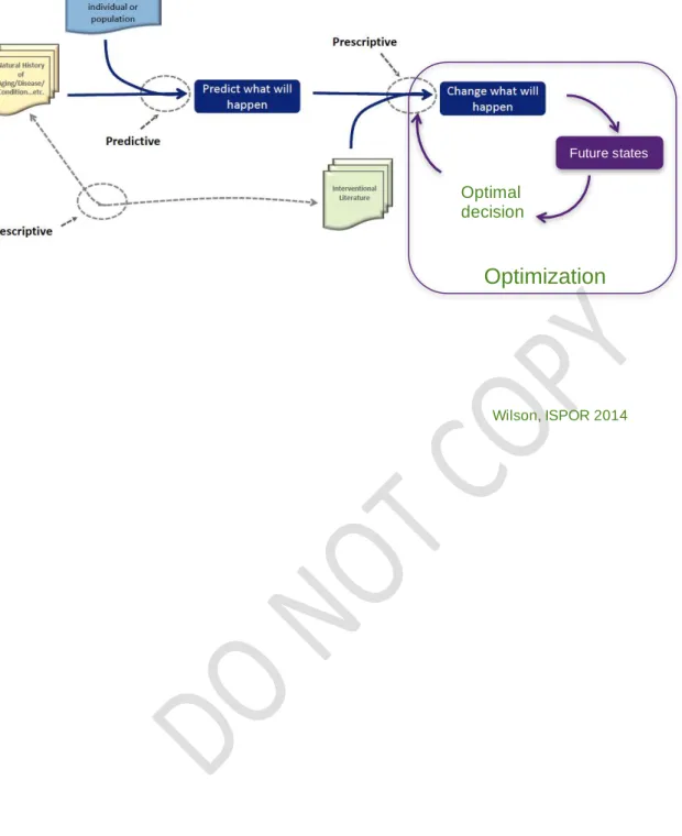
iii.
Prescriptive analytics uses the understanding of systems, both the historical and future based527
on historical (descriptive) and predictive analytics respectively to determine future course of
528
action/decisions. Traditional (without optimization) clinical trials and interventions fall under
529
the category of prescriptive analytics (“Change what will happen” in figure). Constrained 530
optimization is a specialized form of prescriptive analytics, since it helps with determining the
531
optimal decision or course of action in the presence of constraints
532
(https://www.informs.org/Sites/Getting-Started-With-Analytics/Analytics-Success-Stories).
533
14
Figure 2. Descriptive, Predictive, and Prescriptive Analytics. 535
536
7. Summary and Conclusions 537
538
This is the first report of the ISPOR Constrained Optimization Methods Emerging Good Practices Task
539
Force. It introduces readers to the application of constrained optimization methods to health care systems
540
and patient outcomes research problems. Such methods provide a means of identifying the best policy
541
choice or clinical intervention given a specific goal and given a specified set of constraints. Constrained
542
optimization methods are already widely used in health care in areas such as choosing the optimal location
543
for new facilities, making the most efficient use of operating room capacity, etc.
544
However, they have been less widely used for decision making about clinical interventions for patients.
545
Constrained optimization methods are highly complementary to traditional health economic modeling
546
methods and dynamic simulation modeling—providing a systematic and efficient method for selecting the
547
best policy or clinical alternative in the face of large numbers of decision variables, constraints, and
548
potential solutions. As health care data continues to rapidly evolve in terms of volume, velocity, and
549
complexity, we expect that machine learning techniques will also be increasingly used for the development
550
of models that can subsequently be optimized.
551
In this report, we introduce readers to the vocabulary of constrained optimization models and outline a
552
broad set of models available to analysts for a range of health care problems. We illustrate the
553
formulation of a linear program to maximize the health benefit generated in treating a mix of “regular”
554
and “severe” patients subject to time and budget constraints and solve the problem graphically. Although
555
simple, this example illustrates many of the key features of constrained optimization problems that would
556
commonly be encountered in health care.
557
In the second task force report, we describe several case studies that illustrate the formulation, estimation,
558
evaluation, and use of constrained optimization models. The purpose is to illustrate actual applications of
559
constrained optimization problems in health care that are more complex than the simple example
560
described in the current paper and make recommendations on emerging good practices for the use of
561
optimization methods in health care research.
562
15 REFERENCES
564
[1] Rais A, Viana A. Operations research in healthcare: a survey. International transactions in operational 565
research. 2011; 18: 1-31. 566
[2] Araz C, Selim H, Ozkarahan I. A fuzzy multi-objective covering-based vehicle location model for emergency 567
services. Computers & Operations Research. 2007; 34: 705-26. 568
[3] Bruni ME, Conforti D, Sicilia N, et al. A new organ transplantation location allocation policy: a case study of 569
Italy. Health care management science. 2006; 9: 125-42. 570
[4] Ndiaye M, Alfares H. Modeling health care facility location for moving population groups. Computers & 571
Operations Research. 2008; 35: 2154-61. 572
[5] Verter V, Lapierre SD. Location of preventive health care facilities. Annals of Operations Research. 2002; 573
110: 123-32. 574
[6] Lagrange JL. Théorie des fonctions analytiques: contenant les principes du calcul différentiel, dégagés de 575
toute considération d'infiniment petits, d'évanouissans, de limites et de fluxions, et réduits à l'analyse 576
algébrique des quantités finies. Ve. Courcier, 1813. 577
[7] Dantzig GB. Programming of interdependent activities: II mathematical model. Econometrica, Journal of 578
the Econometric Society. 1949: 200-11. 579
[8] Dantzig GB. Linear Programming and Extensions, Princeton, 1963. DantzigLinear Programming and 580
Extensions1963. 1966. 581
[9] Gass SI, Assad AA. An annotated timeline of operations research: An informal history. Springer Science & 582
Business Media, 2005. 583
[10] Kirby MW. Operational research in war and peace: the British experience from the 1930s to 1970. Imperial 584
College Press, 2003. 585
[11] Wood MK, Dantzig GB. Programming of interdependent activities: I general discussion. Econometrica, 586
Journal of the Econometric Society. 1949: 193-99. 587
[12] Burke EK, Causmaecker PD, Petrovic S, et al. Metaheuristics for handling time interval coverage constraints 588
in nurse scheduling. Applied Artificial Intelligence. 2006; 20: 743-66. 589
[13] Cheang B, Li H, Lim A, et al. Nurse rostering problems a bibliographic survey. European Journal of 590
Operational Research. 2003; 151: 447-60. 591
[14] Lin R-C, Sir MY, Pasupathy KS. Multi-objective simulation optimization using data envelopment analysis and 592
genetic algorithm: Specific application to determining optimal resource levels in surgical services. Omega. 593
2013; 41: 881-92. 594
[15] Lin R-C, Sir MY, Sisikoglu E, et al. Optimal nurse scheduling based on quantitative models of work-related 595
fatigue. IIE Transactions on Healthcare Systems Engineering. 2013; 3: 23-38. 596
[16] Sir MY, Dundar B, Steege LMB, et al. Nurse patient assignment models considering patient acuity metrics 597
J -48.
598
[17] Alistar SS, Long EF, Brandeau ML, et al. HIV epidemic control-a model for optimal allocation of prevention 599
and treatment resources. Health Care Manag Sci. 2014; 17: 162-81. 600
[18] Earnshaw SR, Dennett SL. Integer/linear mathematical programming models. Pharmacoeconomics. 2003; 601
21: 839-51. 602
[19] Earnshaw SR, Richter A, Sorensen SW, et al. Optimal allocation of resources across four interventions for 603
type 2 diabetes. Medical Decision Making. 2002; 22: s80-s91. 604
[20] L A S SL H KA A CDC HIV U
605
States. Health care management science. 2011; 14: 115-24. 606
[21] Stinnett AA, Paltiel AD. Mathematical programming for the efficient allocation of health care resources. 607
Journal of Health Economics. 1996; 15: 641-53. 608
[22] Thomas BG, Bollapragada S, Akbay K, et al. Automated bed assignments in a complex and dynamic hospital 609
environment. Interfaces. 2013; 43: 435-48. 610
[23] Zaric GS, Brandeau ML. A little planning goes a long way: multilevel allocation of HIV prevention resources. 611
Medical Decision Making. 2007; 27: 71-81. 612
[24] Lee EK, Wu T-L. Disease Diagnosis: Optimization-Based Methods. 2009. 613
[25] Liberatore MJ, Nydick RL. The analytic hierarchy process in medical and health care decision making: A 614
literature review. European Journal of Operational Research. 2008; 189: 194-207. 615
[26] Ehrgott M, Güler Ç, Hamacher HW, et al. Mathematical optimization in intensity modulated radiation 616
16
[27] Lee H, Granata KP, Madigan ML. Effects of trunk exertion force and direction on postural control of the 618
trunk during unstable sitting. Clinical Biomechanics. 2008; 23: 505-09. 619
[28] Bertsimas D, Farias VF, Trichakis N. Fairness, efficiency, and flexibility in organ allocation for kidney 620
transplantation. Operations Research. 2013; 61: 73-87. 621
[29] Thokala P, Dixon S, Jahn B. Resource modelling: the missing piece of the HTA jigsaw? PharmacoEconomics. 622
2015; 33: 193-203. 623
[30] Marshall DA, Burgos-Liz L, IJzerman MJ, et al. Selecting a dynamic simulation modeling method for health 624
care delivery research Part 2: report of the ISPOR Dynamic Simulation Modeling Emerging Good Practices 625
Task Force. Value in health. 2015; 18: 147-60. 626
[31] Marshall DA, Burgos-Liz L, IJzerman MJ, et al. Applying dynamic simulation modeling methods in health 627
care delivery research the simulate checklist: report of the ispor simulation modeling emerging good 628
practices task force. Value in health. 2015; 18: 5-16. 629
[32] Marshall DA, Burgos-Liz L, Pasupathy KS, et al. Transforming Healthcare Delivery: Integrating Dynamic 630
Simulation Modelling and Big Data in Health Economics and Outcomes Research. PharmacoEconomics. 631
2016; 34: 115-26. 632
[33] Hillier FS. Introduction to operations research. Tata McGraw-Hill Education, 2012. 633
[34] Minoux M. Mathematical programming: theory and algorithms. John Wiley & Sons, 1986. 634
[35] Puterman ML. Markov decision processes: discrete stochastic dynamic programming. John Wiley & Sons, 635
2014. 636
[36] Winston WL, Goldberg JB. Operations research: applications and algorithms. Duxbury press Belmont, CA, 637
2004. 638
[37] Kelley CT. Iterative methods for optimization. Siam, 1999. 639
[38] Kuhn H, Tucker A. Proceedings of 2nd Berkeley Symposium. Berkeley: University of California Press, 1951. 640
[39] Branke J, Deb K, Miettinen K, et al. Multiobjective optimization: Interactive and evolutionary approaches. 641
Springer, 2008. 642
[40] Miettinen K. Nonlinear multiobjective optimization. Springer Science & Business Media, 2012. 643
[41] Drummond MF, Sculpher MJ, Claxton K, et al. Methods for the economic evaluation of health care 644
programmes. Oxford university press, 2015. 645
[42] Chalabi Z, Epstein D, McKenna C, et al. Uncertainty and value of information when allocating resources 646
within and between healthcare programmes. European journal of operational research. 2008; 191: 530-39. 647
[43] Epstein DM, Chalabi Z, Claxton K, et al. Efficiency, Equity, and Budgetary Policies Informing Decisions Using 648
Mathematical Programming. Medical Decision Making. 2007; 27: 128-37. 649
[44] McKenna C, Chalabi Z, Epstein D, et al. Budgetary policies and available actions: a generalisation of decision 650
rules for allocation and research decisions. Journal of health economics. 2010; 29: 170-81. 651
[45] Morton A. Aversion to health inequalities in healthcare prioritisation: A multicriteria optimisation 652
perspective. Journal of health economics. 2014; 36: 164-73. 653
[46] Morton A, Thomas R, Smith PC. Decision rules for allocation of finances to health systems strengthening. 654
Journal of Health Economics. 2016; 49: 97-108. 655
[47] V W G W WH A EM A
656
evaluations in healthcare. Health economics. 2012; 21: 270-81. 657
[48] Tappenden P, Chilcott J, Brennan A, et al. Whole disease modeling to inform resource allocation decisions 658
in cancer: a methodological framework. Value in Health. 2012; 15: 1127-36. 659
[49] Vanderby SA, Carter MW, Noseworthy T, et al. Modelling the complete continuum of care using system 660
dynamics: the case of osteoarthritis in Alberta. Journal of Simulation. 2015; 9: 156-69. 661
[50] Kim E. Sequential drug decision problems in long-term medical conditions: A Case Study of Primary 662
Hypertension. University of Sheffield, 2015. 663
[51] Tosh J. Simulation optimisation to inform economic evaluations of sequential therapies for chronic 664
conditions: a case study in Rheumatoid Arthritis. University of Sheffield, 2015. 665
[52] Banks J. Handbook of Simulation. Wiley Online Library, 1998. 666
[53] Harrison JR, Lin Z, Carroll GR, et al. Simulation modeling in organizational and management research. 667
Academy of Management Review. 2007; 32: 1229-45. 668
[54] Sokolowski JA, Banks CM. Principles of modeling and simulation: a multidisciplinary approach. John Wiley & 669
17
[55] Macal CM, North MJ, Collier N, et al. Modeling the transmission of community-associated methicillin-671
resistant Staphylococcus aureus: a dynamic agent-based simulation. Journal of translational medicine. 672
2014; 12: 1. 673
[56] Milstein B, Homer J, Briss P, et al. Why behavioral and environmental interventions are needed to improve 674
health at lower cost. Health Affairs. 2011; 30: 823-32. 675
[57] Troy PM, Rosenberg L. Using simulation to determine the need for ICU beds for surgery patients. Surgery. 676
2009; 146: 608-20. 677
[58] Sterman JDJD. Business dynamics: systems thinking and modeling for a complex world. 2000. 678
[59] Crown WH. Potential application of machine learning in health outcomes research and some statistical 679
cautions. Value in Health. 2015; 18: 137-40. 680
[60] Kubat M. An Introduction to Machine Learning. Springer, 2015. 681
[61] Witten IH, Frank E. Data Mining: Practical machine learning tools and techniques. Morgan Kaufmann, 2005. 682
683
18
Figure 1. Graphical Representation of Solving a Simple Integer Programming Problem 685
686
687
688
19
Figure 2. Descriptive, Predictive, and Prescriptive Analytics. 690
691
692
693
Wilson, ISPOR 2014 Future states
Optimal decision
20 Table 1. Model Summary and Extensions 694
695
696
Hypothetical problem Real-life Health Services Terminology
Aim Maximize health/health care benefits
Maximize health/health care benefits
Objective function
Options available
Regular or severe patients Service lines, case mix, service mix, etc.
Decision variables
Constraints Total cost < $15 Total time < 1 hour
Budget constraint Time constraint
Resource constraint (e.g. staff, beds, etc.)
Constraints
Evidence base
Cost of each patient, health benefits of each patient and the time taken for consultation
Costs, health benefits, and other relevant data associated with each intervention to be selected
Model (to determine the objective function and constraints)
Complexity Static
The problem does not have a time component; decision made in one time period does not affect decisions made in another
Deterministic
All the information is assumed to be certain (e.g Cost of each patients, health benefits of each patient and the time taken for consultation)
Linear (i.e. each
additional patient costs the same and achieves same health benefits)
Integer/discrete The decision variables (number of patients) can only take discrete and integer values
Dynamic
The optimization problem and parameters may change in different time points, and the decision made at any point in time can affect decisions at later time points (e.g. there can be a capacity constraint defined on 2 months, whereas the planning cycle is 1 month)
Stochastic
Know that the information is uncertain (i.e. uncertainty in the costs and benefits of the interventions)
Non-linear (objective function or constraints may have a non-linear relationship with the model parameters, e.g. total costs and QALYs typically have a non-linear relationship with the model parameters)
Continuous
The decision variables can take fractional values (e.g. number of hours)