Graph similarity through entropic manifold alignment

This is a repository copy of

Graph similarity through entropic manifold alignment

.

White Rose Research Online URL for this paper:

http://eprints.whiterose.ac.uk/112399/

Version: Accepted Version

Article:

Escolano, Francisco, Lozano, Miguel Angel and Hancock, Edwin R

orcid.org/0000-0003-4496-2028 (2017) Graph similarity through entropic manifold

alignment. SIAM Journal on Imaging Sciences. pp. 942-978. ISSN 1936-4954

https://doi.org/10.1137/15M1032454

[email protected] https://eprints.whiterose.ac.uk/

Reuse

Items deposited in White Rose Research Online are protected by copyright, with all rights reserved unless indicated otherwise. They may be downloaded and/or printed for private study, or other acts as permitted by national copyright laws. The publisher or other rights holders may allow further reproduction and re-use of the full text version. This is indicated by the licence information on the White Rose Research Online record for the item.

Takedown

If you consider content in White Rose Research Online to be in breach of UK law, please notify us by

ALIGNMENT

FRANCISCO ESCOLANO∗_{, EDWIN R. HANCOCK}†_{, AND MIGUEL A. LOZANO}‡

Abstract. In this paper we decouple the problem of measuring graph similarily into two

se-quential steps. The first step is the linearization of the Quadratic Assignment Problem (QAP) in a low dimensional space, given by theembedding trick. This is followed by the second step which is the evaluation of an information-theoretic distributional measure which relies on deformable mani-fold alignment. The proposed measure is a normalized conditional entropy, which induces a positive definite kernel when symmetrized. We use bypass entropy estimation methods to compute an ap-proximation of the normalized conditional entropy. Our approach, which is purely topological (i.e. it does not rely on node or edge attributes although it can potentially accommodate them as additional sources of information) is competitive with state-of-the-art graph matching algorithms as sources of correspondence-based graph similarity, but its complexity is linear instead of cubic (although the complexity of the similarity measure is quadratic). We also determine that the best embedding strategy for graph similarity is provided by commute time embedding and we conjecture that this is related to its inversibility property, since the inverse of the embeddings obtained using our method can be used as a generative sampler of graph structure.

Key words. Graph similarity, Graph matching, Graph embedding, Graph Kernels,

Non-parametric Entropy Estimation.

AMS subject classifications.68T45, 05C85

1. Introduction.

1.1. Motivation and Previous Work. The accurate and effective measure-ment of graph similarity has proved to be a challenging problem in structural pattern recognition. Since state-of-the-art methods for object matching aim at incorporat-ing structural information, advances in measurincorporat-ing graph-similarity are pivotal to the development of successful object retrieval techniques. The problem of quantifying graph-similarity has exercised researchers for over three decades. Early approaches included the work of Fischler and Elschlager [21] who exploited an elastic spring analogy, and Barrow and Poppleston’s work [3] based on cliques of the association graph. In the late 1980’s [19], with the emergence of structural pattern recognition as a distinct field of study, several attempts were made to extend the concept of edit distance from strings to graphs and trees. Here Fu and his co-workers [45], showed how to associate edit costs with the insertion, deletion and relabelling of nodes and edges, and developed greedy algorithms to find optimal matches. At about the same time Shapiro and Haralick [46] developed an elegant framework based on consistent clique counting, and Bunke [7] used the maximum common subgraph to define the edit distance between graphs. However, these approaches are based on goal directed considerations motivated by graph theory, and are not information theoretic. One of the earliest attempts to draw on information theoretic concepts to measure graph similarity was presented by Boyer and Kak [6] who exploited the concept of mutual

∗_{Department of Computer Science and Artificial Intelligence, University of Alicante, Alicante,} Spain, 03690 ([email protected]). Supported by the project TIN2012-32839 of the Spanish Govern-ment. Questions, comments, or corrections to this document may be directed to that email address. †_{Department of Computer Science, University of York, Deramore Lane, YO10 5GH, York, UK.} ([email protected]). Supported by a Royal Society Wolfson Research Merit Award .

‡_{Department of Computer Science and Artificial Intelligence, University of Alicante, Alicante,} Spain, 03690 ([email protected]). Supported by the project TIN2012-32839 of the Spanish Govern-ment

information. Christmas, Kittler and Petrou [11] and Wilson and Hancock [53] later showed how relaxation labelling could be applied to the graph matching problem by modelling the probability distribution for matching errors using simple error models. Drawing on ideas from the connectionist literature, Gold and Rangarajan [22] devel-oped a relaxation scheme based on soft-assign, and Finch, Wilson and Hancock [20] took this work one step further by using ideas from statistical mechanics to develop a non-linear version of Gold and Rangarajan’s method. A Bayesian model has been designed for learning generative models using minimum description length, and has exploited the model to compute information theoretic edit distances [50].

There has recently been renewed interest in the graph-matching problem, stim-ulated in part by developments in object retrieval. Here a number of authors have attempted to extend the matching process to incorporate higher order relations. Zass

et al. [55] are among the first to investigate this problem by introducing a probabilistic hypergraph matching framework, in which higher order relationships are marginalized to unary order. Chertok et al. [9] improved this work by marginalizing the higher order relationships to be pairwise and then adopt pairwise graph matching methods. However, these two methods only approximate the hypergraph representation by using a clique graph. It has already been pointed out in [1] that this graph approximation is just a low pass representation of the original hypergraph and causes information loss and inaccuracy. On the other hand, Duchenneet al. [14] have developed the spectral technique for graph matching [29] into a higher order matching framework using the so calledtensor power iteration. Although they adopt anL1norm constraint in

com-putation, the original objective function is subject to anL2norm and does not satisfy

the basic probabilistic properties. The methods described by Shapiro and Brady and Umeyama can be interpreted as implicit embedding methods, while the more recent methods of Caelli and Kosinov [8] and Robles-Kelly and Hancock [44] make use of explicit embeddings. However, one of the weaknesses of these methods is that they are again not information theoretic in their development.

More recently, the factorized/deformable graph matching (FGM/DGM) approach proposed in [56][57] has uncovered the interplay between the topological information derived from node attributes and the attributes themselves. In this way, a unified approach to graph matching has been proposed, using a convex-concave relaxation of the quadratic assignment problem, similar to that used in the well known path-following algorithm [54].

1.2. Contributions. In this paper, we decouple the problem of computing graph similarity into that of solving an approximate graph matching problem, followed by the estimation of an information-theoretic similarity measure computed from the available matching. This decoupling is motivated by the need to reduce the cubic complexity of state-of-the-art graph matching algorithms. We avoid measuring graph similarity in terms of the number of correct correspondences, which forces the con-tinuous improvement of polynomial solutions to the quadratic assignment problem (QAP). Instead, we turn our attention to solving a linearized version of the QAP in an embedding space (we exploit the embedding trick) and then use this solution to estimate a highly discriminative graph similarity measure. In this paper, we define the conditions that must be satisfied for a graph embedding to be a good linearizer of the QAP problem, namely (a) the dimensionality is bounded by the intrinsic dimension, (b) it approximates the geodesic with a L2 norm, and (c) the manifold embedding

We show that despite being a fairly rough approximation of the QAP solution, the linearized solution obtained has sufficient inliers to support a low-energy global transformation between the manifolds induced by the embeddings. Such a transfor-mation imitates the topological regularizing role of the QAP cost function (via the rectangle rule) but in a geometric space. Given this transformation, the computation of graph similarity is posed in terms of a normalized conditional entropy between the aligned manifolds. In this way we account for the high order statistical dependen-cies between the sampled manifolds. We prove that the similarity measure obtained induces a positive definite kernel.

The remainder of this paper is organized as follows. In Section 2 we define the lin-earized version of QAP referred to as Structural Embedding Graph Matching (SEgm). SEgm ispurely topological, i.e. it relies exclusively on the adjacency matrices of the graphs being matched, although it can also additionally accommodate attributes com-ing from edges or node characteristics, dependcom-ing on the application domain. This purely topological approach allows us to understand the power of the embedding trick without relying on node or edge attributes. Significantly, it paves the way to a distribu-tionalgraph similarity measure, the so callednormalized squared conditional entropy

(NSCE). We detail the NSCE in Section 3 and we also prove that its symmetrized ver-sion is a positive definite kernel. Section 4 is devoted to approximating the kernel with a bypass entropy estimator. This requires that we perform some simplifications for the sake of efficiency. Then, in Section 5 we validate our approach through (a) testing the proposed strategy oflinearization + similarity, referred to asEntropic Alignment

or EA (see Fig. 1) on a standard database (Houses Images dataset), (b) evaluating alternative information-theoretic measures and embeddings for a more challenging database (Gator), (c) comparing with alternative algorithms, specifically FGM/DGM and path-following, in terms of graph retrieval performance for both databases. From the experiments, we conclude that our strategy is competitive with FGM/DGM and path-following. Moreover, the best performance is provided when the commute time embedding is used in the linearized step. In Section 6 we formulate the problem of inverse embedding and prove that the commute time embedding is reversible. We conjecture that the success of such an embedding may be motivated by this property. Finally, in Section 7 we present our conclusions and suggest directions for future work.

2. Structural Embedding Graph Matching. Let X = (VX, EX) and Y = (VY, EY) be two undirected and unweighted graphs with respective node-setsVXand

VY, edge-setsEX andEY and numbers of nodesn =|VX| and m =|VY|. Also let

fX : VX → Rd and fY : VY → Rd with d ≪ max{n, m} be also two embedding

functionssatisfying:

a) They induce two low-dimensional subspaces (manifolds)MX andMY ofRd wheredis bounded by the intrinsic dimensions of the manifolds.

b) For each pair i, j ∈ VX we have that gX(i, j) ≈ ||fX(i)−fX(j)||2, where

gX(i, j) is the length of the geodesic betweeniandj, and similarly foru, v∈

VY andgY(u, v)≈ ||fY(u)−fY(v)||2.

c) EXansEY can be respectively inferred fromDX ={||fX(i)−fX(j)||2,∀i, j∈

VX}andDY ={||fY(u)−fY(v)||2,∀u, v∈VY}with bounded errorsǫXand

ǫY.

Fig. 1. Entropic Alignment. Top-Left: Inliers provided by SEgm. Top-Right: SEgm formula-tion and manifold alignment. Bottom: After the optimal alignment we proceed to measureSN SCE: inlier correspondences in green, outliers in red and blue; both are used for the KNN estimation of the entropies and then the positive define kernel.

(i.e. characterized by weight matrices WX and WY) and fX, fY will be computed respectively fromAX+αxWX andAY +αyWY,αx>0,αY >0.

Given twoextended graphsGX ={VX, EX,AX, fX}andGY ={VY, EY,AY, fY}, withAX∈ {0,1}n×nandAY ∈ {0,1}m×m, and embeddingsfX,fY with dimension-ality d ≪max{n, m}, the aim of Structural Embedding Graph Matching (SEgm) is to find the one-to-one mapping (matching or correspondence) encoded by a partial permutation matrixX_∈Π, Π ={X_|X_{∈ {}0,1}n×m_,X1

m≤1n,XT1n ≤1m} maxi-mizing

JSEgm(X,T) =tr Kf(T)TX−ψ(T), (2.1)

where:

a) T(.,W) is a global non-rigid transformation parameterized byWandψ(.) is a regularization function typically given byψ(T) =λtr(WTGW) whereG

a Green’s function.

b) Kf_∈Rn×m_{is a structural deformation matrixgiven by}

Kf_iu=||fX(i)− T(fY(u);W)||2,

Therefore, SEgm a can be seen as a linearization of the purely structuralversion of the Quadratic Assignment Problem (QAP), whose objective is to maximize

JQAP(X) =tr KTq GXTXGY ◦HTXXHY , (2.2)

where: KT_{q ∈} R|EX|×|EY| _{is the edge attributes matrix (only applying when} WX and WY are defined), ◦ is the Hadamard product, and GX ∈ {0,1}n×|EX|, GY ∈

{0,1}m×|EY|_{are thebinarynode-edge incidence matrices (G}ic

X=H

jc

Y = 1 if thec−th edge starts fromi and ends atj, and similarly forGY andHY). Here we follow the Factorized Graph Matching formulation [56].

SEgmrelies on the assumption thatXSEgm, the global optimizer ofJSEgm(X,T) is a reasonable approximation ofXQAP, the global optimizer ofJQAP(X). The error of the approximation depends on two factors:

1. The quality of the embedding trick. Graph embedding methods are de-signed to capture high-order similarities between nodes. If the approximation

gX(i, j) ≈ ||fX(i)−fX(j)||2 is sufficiently good, we capture the long-range interactions between nodes which are by far more informative than the exis-tence of edges and the node degrees. In this regard, theinversibility property

(to what extent the original edges can be recovered from all pairs of Eu-clidean distances ||fX(i)−fX(j)||2) plays a critical role in the effectiveness of an embedding for the purposes of graph matching.

2. The regularizing power of T. The apparent simplicity of Kf_iu = ||fX(i)−

T(fY(u);W)||2 is misleading. The role of the non-rigid transformationT in SEgm is purely structural (i.e. it does not rely on node attributes) and it simulates the role of the topological regularization imposed by GT_XXGY ◦

HT_XXHY in QAP. It is well known that the rectangle rule represented by

XiuAijXAuvY Xjv, imposes the constraint that the adjacent nodes i ∈ VX,

j ∈ VX should match adjacent nodes u ∈ VY, v ∈ VY. This is the role of the quadratic cost of QAP and the origin of the NP-hard complexity of graph matching. Similarly, T enforces that the d−dimensional neighbors of both fX(j) ∈ MX and fY(v) ∈ MY match if ||fX(i)− T(fY(u);W)||2 is sufficiently small. Therefore, the combinatorial requirements are replaced by the regularizing power of a geometric transformation.

We should not expect the SEgmapproximation to be sufficiently good for low-error correspondence recovery, even after a careful choice of the embedding and the regu-larizer. The reason for this is that the above linearization resembles that used in Deformable Graph Matching (DGM) [57], and which is designed for graph recovery. If our final objective is graph recovery or classification, thenSEgmprovides a set of inliers supporting the global alignment of MX and MY. Given such an alignment, it leads to a similarity measure that is sufficiently discriminative to work effectively since such similarity isdistributional.

3. The SN SCE Distributional Graph Similarity. Let ΘX and ΘY be two random variables whose realizations are points in Rd _{belonging to MX and MY} respectively. Then, the conditional probability of observing ΘX given ΘY after the alignmentT(.;W) can be modeled by the factorization

p(ΘX|ΘY,T) = m

Y

u=1

where

pu(fX(c(u)|fY(u),T)∝exp−1 2

(

fX(c(u))− T(fY(u);

W)

σ

2)

,

(3.2)

where i ∈ VX, u ∈VY are graph nodes, c : VY → VX is a correspondence function given by the optimal solution of the Structural Embedding Graph Matching Problem

(SEgm), andσa bandwidth parameter determined during the alignment. The band-width parameterσis proportional to the global error, i.e. σ∝Pni=1

Pm

u=1||fX(i)− T(fY(u)W)||2=Pi

P

jK

f

iu, whereK f

iu is the structural deformation matrix. Given the conditional density p(ΘX|ΘY,T) our similarity function relies on the contitional entropyH(p(ΘX|ΘY,T)) defined as:

H(p(ΘX|ΘY,T))≈Hˆ(p(ΘX))−Hˆ(p(ΘX|ΘY,T)) , (3.3)

where H(.) denotes the Shannon entropy and ˆH(.) is an estimator of the R´enyi en-tropy [28] whose limit is the Shannon enen-tropy. As we will see later in Section 4, it is the choice of estimators of the R´enyi type that validates the approximation in Eq. 3.3. Then, thenormalized conditonal entropybetween two random variables ΘY and ΘX after the alignment is given by

¯

H(ΘX|ΘY,T) = ˆ

H(p(ΘX))−Hˆ(p(ΘX|ΘY,T)) ˆ

H(p(ΘX)) + ˆH(p(ΘX|ΘY,T))

,

(3.4)

Then, ¯H(ΘX|ΘY,T) has the following properties:

a) The numerator is the conditional entropyH(p(ΘX|ΘY,T)) between the (sam-pled) manifolds given the transformationT, i.e. it is the reduction in entropy ofp(ΘX) after the alignment. If the alignment provides two identical mani-folds then the conditional entropy is zero.

b) Normalization by ˆH(p(ΘX))+ ˆH(p(ΘX|ΘY,T)) is key when we compare man-ifolds induced by graphs with a significantly different number of nodes. We prefer this form of the numerator to the alternative ˆH(p(ΘX)) + ˆH(p(ΘY)), since it enforces the role of the conditional probability and the transformation. c) ¯H(ΘX|ΘY,T) isdirectional, i.e. T : ΘY →ΘXso thatpu(fX(c(u)|fY(u),T)>

0 whenever it is possible given the smoothness constraint imposed by the min-imization ofψ(T).

The above properties lead us to define a kernel between the probability functions for the manifolds and, thus, implicitly between the graphs. Such kernels are of pivotal importance for principled comparisons of the probability distributions associated with the manifolds [33]. In this regard, we have that:

• Since the Shannon/R´enyi entropy is negative definite (nd), and negative defi-niteness is closed under the sum, we have that ˆH(p(ΘX)) + ˆH(p(ΘX|ΘY,T)) is nd. Then

1 ˆ

H(p(ΘX)) + ˆH(p(ΘX|ΘY,T)) +a is pd for anya >0 (see Proposition. 20 in [33]).

• Since H(p(ΘX|ΘY,T)) is nd, to ensure positive definiteness we add a non-negative constant and square the alignment-based conditional entropy, i.e.

(H(ΘX|ΘY,T) +b)2=

ˆ

H(p(ΘX))−Hˆ(p(ΘX|ΘY,T)) +b

is pd forb >0.

In addition to the above considerations is the fact that the product of two pd measures is pd, i.e. we have that

K(p(ΘX)|p(ΘY),T) = (H(ΘX|ΘY,T) +b)

2

ˆ

H(p(ΘX)) + ˆH(p(ΘX|ΘY,T)) +a (3.5)

is a pd measure, fora, b >0, between the density functions of ΘX and ΘY. We refer to this measure as theNormalised Squared Conditional Entropy(NSCE) between the two densities, and consequently between the extended graphsGX and GY given the alignmentT.

However, the N SCE is still not a kernel, since it is not symmetric due to the directionality of the transformationT : ΘY →ΘX. Then, letT′ : ΘX →ΘY be the non-rigid transformation given byT′_{= (.;W}′_{). Such a transformation optimizes}

JSEgm(X′,T′) =tr K′f(T′)TX′−ψ(T′), (3.6)

where X′ _{∈ {}0,1}m×n _andK′f _∈Rm×n _{is the structural deformation matrix which} hasuientries given by

K′_uif =||fY(u)− T′(fX(i);W′)||2.

Then, the definition ofp(ΘY|ΘX,T′) in terms ofpui(ΘY|ΘX,T′) gives ¯

H(ΘY|ΘX,T′) = ˆ

H(p(ΘY))−Hˆ(p(ΘY|ΘX,T′)) ˆ

H(p(ΘY)) + ˆH(p(ΘY|ΘX,T′))

,

(3.7)

which in turn leads to

K(p(ΘY)|p(ΘX),T′) =

(H(ΘY|ΘX,T′) +b)2 ˆ

H(p(ΘY)) + ˆH(p(ΘY|ΘX,T′)) +a

.

(3.8)

Finally, the Symmetrized Normalized Squared Conditional Entropy between two ex-tended graphsGX andGY is the pd kernel given by

SN SCE(GX,GY) =K(p(ΘX)|p(ΘY),T) +K(p(ΘY)|p(ΘX),T′).

(3.9)

We can then exploit the kernel trick to classify graphs, and thus recover or recognize objects by their structure, as in [15].

4. Leonenko et al. Entropy Estimator. TheSN SCE(GX,GY) similarity mea-sure isdistributional. Here, the termdistributionalemphasizes the continuous nature of manifoldsMXandMY sampled atfX(i), i∈VX andfY(u), u∈VY. Actually, the computation ofSN SCE(., .) requires, in principle, the estimation of densitiesp(ΘX),

p(ΘY), p(ΘX|ΘY,T) and p(ΘY|ΘX,T′). When dis very low (for example 2D/3D) data we can exploit non-parametric kernel density estimators such as the Parzen win-dows [37]. However, Parzen winwin-dows do not scale well withdand tend to overestimate entropy for medium/high dimensions, which is the case of graph embedding.

Therefore, instead of using a plug-in entropy estimator (inferring the probabil-ity densprobabil-ity function before computing the Shannon entropy), here we use a bypass

X = {1,2,3} Y’=Y+ T={a,b,c} 1 3 2 a c b 1 3 2 c b 1 3 2 c CORRESPONDENCE from SEgm

H(X|Y’=a,T) = logA1’+ logB1’ = logA1’+ logB1’ = log(A-a1) + logB =log(A)+log(1-a1/A) + logB = H(X) + log(1-a1/A) 1 3 2 a A A1’=A-a1

B1’=B

A

B

H(X|Y’=b,T) = logA2’+ logB2’ = log(A-a2)+log(B-b2) = H(x) + log[(1-a2/A)*(1-b2/B)]

A2’=A-a2 B’=B-b2

A3’=A+a3

B’=B+b3

H(X|Y’=b,T) = logA3’ + logB3’ = log(A+a3)+log(B+b3) = H(x) + log[(1+a3/A)*(1+b3/B)] 1 3 2 a c b Dac D13 Dbc D23

H(X|Y’=a,T) = logA1’+ logB1’ = logA1’+ logB1’ = log(A-a1) + logB = log(A)+log(1-a1/A) + logB = H(X) + log(1-a1/A)

H(X|Y’=b,T) = logA2’+ logB2’ = log(A-a2)+log(B-b2) = H(x) + log[(1-a2/A)*(1-b2/B)]

H(X|Y’=b,T) = logA3’ + logB3’ = log(A+a3)+log(B+b3) = H(x) + log[(1+a3/A)*(1+b3/B)]

H(X|Y’,T) = Ey’[H(X|Y’=y’,T)] = H(X) + DefA/N + DefB/N

DefA/N = log[(1-a1/A)*(1-a2/A)*(1+a3/B)]/3 DefB/N = log[(1-b2/A)*(1+b3/B)]/3

_{H(X|Y,’T) = logDac +logDbc = log(A1’+c1) + log(B1’-c2)} = log(A-a1+c1) + log(B-c2)

= H(X) + log(1+(c1-a1)/A1) + log(1-c2/B2) H(X|Y’,T) = Ey’[H(X|Y’=y’,T)] = H(X) + DefA/N + DefB/N

DefA/N = log[(1-a1/A)*(1-a2/A)*(1+a3/B)]/3 DefB/N = log[(1-b2/A)*(1+b3/B)]/3

Estimation From the Average

Estimation ‘Once at a time’

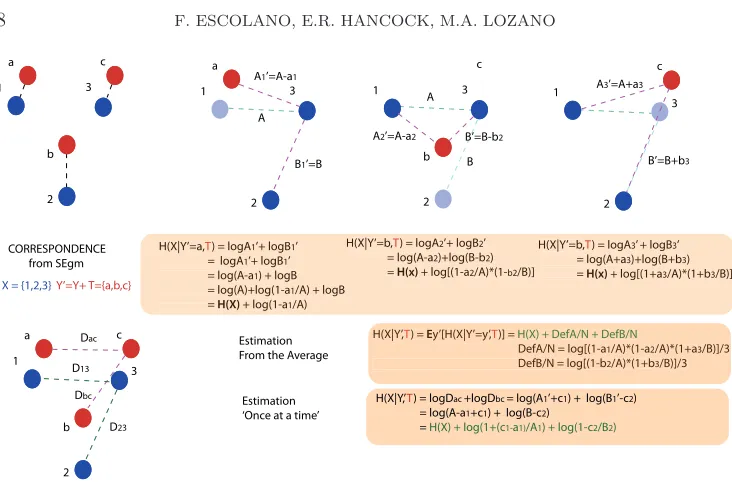
Fig. 2. Estimating Conditional Entropy (toy example). Blue dots are samples of X and red ones are those ofY′ _{=Y +T. After the optimal alignment we proceed to compute Hˆ(X|Y}′_,T). Top-right: we replace eachX y a value ofY′_{and recompute the entropy. R´enyi entropy is encoded} by the neighborhood structures: ofX (in green) and ofX after replacingXi by the corresponding

Yi(magenta). Bottom: the average distortion is similar to that of making all the replacements at a time, and they both depend ofHˆ(X). In all casesk= 1.

estimator [28] and its implications in estimating mutual information (MI) [27], because mutual information satisfies:

I(ΘX,ΘY) =H(ΘX)−H(ΘX|ΘY) =H(ΘY)−H(ΘY|ΘX), (4.1)

that is, it is closely related to conditional probabilities: MI it is the amount of uncer-tainty reduction due to the conditioning. Actually it should be more desirable to use mutual information as a similarity measure instead of conditional entropy. However, the Kozackenko-Leonenko is better adapted to the alternative definitions of MI:

I(ΘX,ΘY|c) =H(ΘX) +H(ΘX)−H(ΘX,ΘY), (4.2)

whereI(ΘX,ΘY) is thejoint entropyandc:VY →VXis the correspondence function. This function is key to construct an estimator of H(ΘX,ΘY) so that the samples

zu = (fX(c(u)), fY(u)) of the variable ZXY = (ΘX,ΘY) are properly built. The correpondence function establishes a common reference system as in the case of image alignment [36][40]. However, the optimal transformationT is no needed here since it is not going to be applied tofY(u) withu∈VY.

However, when applying the Kozackenko-Leonenko/Kraskow et al.’s approach, we obtain the following entropy estimator

ˆ

HN,k,1=−Ψ(k) + Ψ(N) + logVd+ d

N

N

X

i=1

and its associated estimator ofI(ΘX,ΘY;c): ˆ

IN,k,1= Ψ(k)−1

k−Ψ(N)−

1

N

N

X

u=1

(Ψ(nx(c(u)) + Ψ(ny(u))), (4.4)

where: ǫ(i) is twice the Euclidean distance of the i−th point of the manifold to its

k−th neighbor,N is the number of i.i.d. samples ofX′_={f

X(c(u)), c(u)∈VX}and

Y ={fY(u), u∈VY}, i.e. |X′|=|Y|. Letǫx(c(u)) be the distance between fX(c(u)) and itsk−th nearest neighbor inX′_{, and letǫ}

y(u) be the distance betweenfY(u) and itsk−th nearest neighbor in Y (here the max norm is used); thennx(c(u)) andny(u) are respectively the number of points xj ∈ X′ with ||fX(c(u))−xj|| < ǫx(c(u))/2 and the number of points yj ∈ Y with||fY(u)−yj||< ǫy(u)/2. In addition Ψ(k) = Γ′_{(k)/Γ(k) =−γ+Ak}

−1 is the digamma function with γ≈0.5772 (Euler constant)

andA0= 0,Aj=Pji=11/i.

The ˆIN,k,1estimator does not include explicitly the distancesǫx(c(u)) andǫy(u). It embodies these distances in rank data: accounting from the expected number of points surrounding a given one in a ball of radiusǫx(c(u)) orǫy((u)) gives an idea of the amount of joint entropy. However,nx(.) andny(.) are the result of a marginalization of

ǫ(u) (the distance betweenzu= (fX(c(u), fY(u)) and itsk−th nearest neighbor). The marginalization is imposed by the fact that designing a 2dball imposes a neighboring structure quite different from that used for estimating the marginal entropies and this leads to larger systematic errors when dgrows becauseǫ(u) tends to be much larger than the marginals. As a result, our experiments included in Section 5 show that the

ˆ

IN,k,1 estimator leads to a poor discrimination.

As an alternative, theSymmetrized Normalized Squared Conditional Entropy(Eq. 3.9) relies on the conditional entropyH(ΘX|ΘY,T) (see Eq. 3.3). Despite the conditional entropy is less effective than the MI for pattern discrimination, it is better adapted than MI when the Kozackenko-Leonenko/Kraskow et al.’s estimator is used. This is due to the following properties:

a) We avoid the marginalization of ǫ(u) while preserving the consistency of the estimator. This is ensured by the compatibility of the ranges associated both with the samples ofX = ΘX and those ofZX|Y = (ΘX|ΘY,T).

b) We choose the samples forZX|Y = (ΘX|ΘY,T) so that they are compatible with the conditional entropyH(ΘX|ΘY,T)in conjunctionwith the samples ofX = ΘX.

To commence, let us characterize theentropy conditioninginRd_{in terms of replacing} each pointfX(c(u)) by its corresponding pointfY(u)′=fY(u) +T after the transfor-mationT and then computing an entropy. The average of thementropies is a proper approximation of the conditional entropy, since:

H(ΘX|ΘY,T) = m

X

u=1

p(ΘX)H(ΘX|ΘY =fY(u)′,T) (4.5)

≈_m1

m

X

u=1

H(ΘX|ΘY =fY(u)′,T)

≈ C

m

m

X

u=1

ˆ

Hm,k,1({ΘX∼fX(c(u))} ∪ {fY(u)′})

.

= C

m

m

X

u=1

ˆ

whereC is a constant. It can be proved that C m m X u=1 ˆ

Hm,k,1(X|u) =Hm,k,1(ΘX) +C

X e E_u log

1±δe |e|

,

(4.6)

where eare the edges of thek−th neighborhood system of the points of ΘX (see an example in Fig. 2 where we drop C for the sake of clarity). We denote by |e| the length of the edges and by δethe difference between their original lengths |e|when a new point of ΘY is introduced. ThenEu(log (1±δe/|e|)) is the expectation of the log-relative errors for each edge over all choices ofudefining fY(u)′. We refer to this approximation asestimation from the average.

However, if we fix the edgeseof ΘX and express thosee′ of ΘY in terms ofewe have that

ˆ

Hm,k,1(ΘY′)≈Hm,k,1(ΘX) +C

X

e log

1±δ

2_e

|e|

,

(4.7)

i.e. each expectation can be approximated by the log of a second-order error (as in the variance). This leads to the following approximation of the conditional entropy:

H(p(ΘX|ΘY,T))≈Hm,k,1(ΘX)−Hˆm,k,1(ΘY′) =K

X

e log

1±δ

2_e

|e|

.

(4.8)

This approximation can be interpreted in terms of a sum of log-likelihood ratios since forn=m we have that for the Leonenko et al.’s entropy estimator [28] used in this paper (see more details in Appendix A):

H(p(ΘX|ΘY,T)) = ˆHm,k,2(X)−Hˆm,k,2(Y′)

(4.9)

= −Ψ(_mk)+log(m−1)

m + logVd+ d

2m

m

X

i=1

logǫX(i)

+Ψ(k)

m −

log(m−1)

m −logVd− d

2m

m

X

u=1

logǫY′(u)

! = d 2m m X i=1

log ǫX(i)

ǫY′(u)

,

where i = c(u), and ǫX(.), ǫY′(.) are respectively twice the distances to the k−th neighbor of the point i=c(u) ofX and of the k−th neighbor of the u−thpoint of

Y′ _{. The Euclidean norm is used in order to avoid the marginalization ofǫ(.). When}

m6=nwe have either positive or negative deviations/penalizations from this sum of log-likelihood ratios. Our estimator measures the neighborhood distortion and this distortion is highly compatible, through not exactly so, with the conditional definition of entropy. For instance, when ΘX= Θ′Y we have that the conditional entropy is zero as expected. Furthermore, in this way conditional entropy is consistent with the concept ofapproximate entropyinsofar it captures incremental variations [38].

Consequently, we then use the approximation in Eq. 4.9 (replacing ˆHm,k,1 by

ˆ

Hm,k,2) to computeSN SCE(GX,GY) (Eq. 3.9).

advances in cryptography [26], where estimating the correct amount of uncertainty is critical, point towards learning techniques that exploit the knowledge available about the random sources (the graphs and the embedding functions). In Section 5.5, where we validate the commute time embedding as the most successful embedding function for graph matching/similarity purposes, we will analyze the impact of this choice in the entropy estimator.

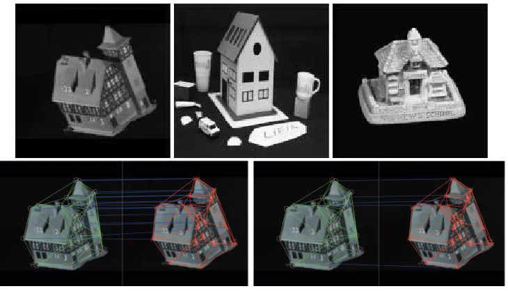
Fig. 3. Houses dataset. Top: from left to right example frames of CMU, MOVI and Chalet/York. Bottom: examples of inliers obtained by SEgm when matching frames 1 and 4 in CMU for different embedding dimensions (d= 4- left, andd= 11- right).

0 6 9 14 19 24 29

20 20.2 20.4 20.6 20.8 21 21.2 21.4 21.6 21.8

Embedding dimension d

Houses AUCs

PERFORMANCE STABILITY

EA’s AUCs Optimal d=6

0 5 10 15 20 25 30

0 0.1 0.2 0.3 0.4 0.5 0.6 0.7 0.8 0.9 1

Retrieval

Average Recall

ALGORITHMS COMPARISON

FGM EA RRW SMAC GA

5 10 15 20 25 30 0.2

0.3 0.4 0.5 0.6 0.7 0.8 0.9 1

Retrieval

Average Recall

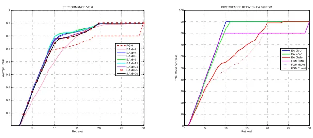
PERFORMANCE VS d

FGM EA d=2 EA d=4 EA d=5 EA d=6 EA d=11 EA d=21 EA d=25 EA d=29

0 5 10 15 20 25 30

0 10 20 30 40 50 60 70 80 90 100

Retrieval

Total Recall per Class

DIVERGENCES BETWEEN EA and FGM

EA CMU EA MOVI EA Chalet FGM CMU FGM MOVI FGM Chalet

Fig. 5.Performance of EA vs FGM . Left: Stability of EA’s AUCs with respect to the embedding dimensiond. Right: Analysis of total recalls for the three houses categories: EA vs FGM.

5. Experimental Results.

5.1. Entropic Alignment Settings. We refer to the proposed strategy of lin-earization + symilarity asEntropic Alignment (EA). In our experiments, Structural Embedding Graph Matching (SEgm) relies on the CPD (Coherent Point Drift) algo-rithm [34] because it generalizes the non-rigid alignment to an arbitrary number of dimensions, sayd, of the input data (manifolds in this case). CPD follows a similar approach to that in [25], where the samples are considered the centers of variance-isotropicd−dimensional Gaussian Mixtures (GMM). For the Leonenko’s entropy es-timator, which is the key element for measuringSN SCE, we setk= 4.

5.2. Houses Images Dataset. The Houses (CMU+MOVI+Chalet) dataset consists of 10 frames of the CMU-VASC sequence1, 10 frames of the INRIA MOVI sequence and another 10 frames of the Swiss chalet sequence created at The Univer-sity of York (UK). These sequences have associated with them 30 graphs (Delaunay triangulations) and they have been tested (totally or partially) in many papers ad-dressingpure topological(attribute-free) graph matching methods (usually of spectral nature) such as [31],[48],[43] and [32]. In Fig. 3-Top we show examples of frames for the three categories, a) CMU, b) MOVI and c) Chalet.

We commence our experimental evaluation with this dataset because the topolog-ical variability increases from CMU to MOVI and Chalet. CMU has low intra-class variability and high inter-class variability, MOVI can be easily discriminated from CMU but confused with Chalet (it is by far more confused with Chalet than CMU). In addition, Chalet is the class with maximal intra-class structural variability and minimal inter-class variability. The number of nodes ranges from 30 to 31 in CMU, 130−141 in MOVI and 40−136 in Chalet.

For the Entropic Alignment (EA) method, the first question to address is the

supporting quality of the inliers provided by Structural Embedding Graph Matching (SEgm). The quality depends on the dimensionality of the embedding d. In Fig. 3-Bottom we show two extremal cases in CMU, where we have ground truth. For a low dimensionality (d= 4) we obtain 10 inliers (1/3 of the matchings), whereas for

d= 11 this number is reduced to 5 (1/6 of the matchings). For each SEgm matching

1

(CM Ui, CM Uj) the number of inliers varies significantly with d, i.e. there is no significant correlation (positive or negative) betweendand the number of inliers for a given pair of matched CMU frames, which can be zero. The number of pooled inliers for (CM Ui, CM Uj) is in the range 98−1061 and in the interval 395.7±205.1. In all these experiments the graph embedding functions fX(.) and fY(.) are given by the commute time (CT) embedding [39].

Despite the high variance in the number of inliers with respect tod, we have that

theSN SCE similarity is quite robust with respect to variations ofd in this dataset.

In Fig. 4-Left, we show the evolution of the Area Under the Curve (AUC) of the Average Recall/Retrieval curves ford in the range 1−29. We found that the most discriminative value ofdfor this dataset isd= 6 (we cannot trust on estimators of the intrinsic dimension since they tend to overestimate due to the curse of dimensionality). In Fig. 4-Right we show that the pure topological version(SEgm based on adja-cency matrices) of EA outperforms state-of-the-art graph matching algorithms such as Factorized Graph Matching (FGM) [56], Spectral Matching with Affine Constraint (SMAC)[13], Reweighted Random Walks [10], Graduated Assignment (GA) [22], when node and/or edge attributes are used and graph similarity relies on their respec-tive cost functions. In Table. 5.2 (wherecomplexityrefers to complexity per iteration, where applicable) we summarize the results obtained for the AUCs of such algorithms. It is important to stress that, despite the best result for EA is provided byd= 6 (the optimal choice), we have that even with the minimald= 2 EA outperforms the second best alternative (Factorized Graph Matching) in terms of AUC. This reveals that the choice ofdis not critical in this dataset.

A more detailed analysis of the curves in Fig. 5-Right reveals that EA withd= 6 outperforms FGM even for a small number of retrievals. Since the Average Re-call/Retrieval curves show how the performance improves when an increasing number of examples are considered for evaluation, we found that EA begins to improve the FGM method after only 3 retrievals.

The performance stability of EA with respect to d is detailed in Fig. 5-Left, where we show the Average Recall/Retrieval curves of EA for different values of d. The curve for EA is only below that for FGM for d = 2. Close to the optimal value d = 6 AUC is maximal and decreases slightly for higher dimensions. The performance of the FGM method diverges significantly from that obtained with EA after 9 retrievals ford >2, and later (12 retrievals) ford= 2. A closer class-by-class

analysis of the divergence (see Fig. 5-Right) reveals that FGM is competitive (up to 10 retrievals) when discriminating classes CMU and MOVI. After 10 retrievals we find that there is a constant gap between EA and FGM for these classes. This is mainly attributable to the fact that the quadratic cost function of FGM induces significantly more intra-class variability than EA when measuring the similarity between examples of CMU and MOVI. However, the main bulk of the performance divergence comes from the fact that FGM poorly discriminates the most structurally complex class, Chalet, from CMU and MOVI (at least such discrimination is worse than that given by EA). This means that EA is able to deal with high intra-class variability and low inter-class variability. FGM, on the other hand, basically relies on the number of correspondences and the associative effects of the rectangle rule, and is limited by the size of the smallest graphs in each class. This is why in CMU data, where all graphs have close to 30 nodes, FGM is (to some extent) competitive.

section we focus our analysis on the differences between both algorithmswhen only topological information is used. To this end, we need a more complex and challenging dataset which is provided by the Gator database.

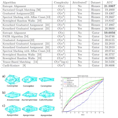
Table 1

Summary of Experiments with Houses and Gator

Algorithm Complexity Attributed? Dataset AUC

Entropic Alignment O(n) No Houses 21.5967

Factorized Graph Matching[56] O(n3_{) Yes Houses 19.4800}

Graduated Assignment[22] O(n4_{) Yes Houses 19.4367}

Spectral Maching with Affine Const.[13] O(n2_{) Yes Houses 19.2667}

Reweighted Random Walks [10] O(m2) Yes Houses 18.8167

Kernelized Graduated Assignment [31] O(n4_{) No Houses 17.4867}

Kernelized Graduated Assignment [31] O(n4_{) Yes Houses 20.9600}

Entropic Alignment O(n) No Gator 59.6056

PATH Algorithm[54] O(n3_{) No Gator 58.6746}

Graduated Assignment[22] O(n4_{) No Gator 39.6155}

Kernelized Graduated Assignment [31] O(n4_{) No Gator 33.2810}

Kernelized Graduated Assignment [31] O(n4_{) Yes Gator 53.2810}

Spectral Maching with Affine Const.[13] O(n2_{) Yes Gator 49.0744}

Reweighted Random Walks [10] O(m2_{) Yes Gator 46.3757}

Reweighted Random Walks [10] O(m2_{) No Gator 46.0969}

Tensor-Based Matching [14] O(n3_{logn) Yes Gator 50.5456}

Caelli-Kosinov [8] O(n3_{) No Gator 39.8606}

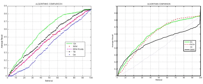
Fig. 6.Examples of the Gator database (left) and average recall curves (right)

5.3. The Gator Dataset. The Gator 100 Dataset is a topological version of the UCF Fish Shape Database2_{. It consists of 100 Delaunay triangulations extracted}

from images of fishes drawn from 30 different classes (see Table 2 where vertical lines separate examples of different classes). Since the classes are associated to fish genus and not to species, we find high intra-class variability – see a) in Fig. 6-Left where the

2

Table 2

Graphs based on Delaunay triangulations for the Gator Database

corresponding class has 8 species. There are also very similar species from different classes (row b)) and few homogeneous classes (row c)). There are 10 classes with one species, and these are not included in the analysis and performance curves. There are 11 with 1−3 individuals, 5 with 4−6 individuals and only 4 classes with more than 6 species.

ex-0 10 20 30 40 50 60 70 80 90 100 0

0.1 0.2 0.3 0.4 0.5 0.6 0.7 0.8 0.9 1

CONDITIONAL VS MI ESTIMATION

Retrieval

Average Recall

Conditional (EA) Conditional (Union) MI Kraskow (no T) MI Kraskow (after T)

0 10 20 30 40 50 60 70 80 90 100 0

0.1 0.2 0.3 0.4 0.5 0.6 0.7 0.8 0.9

Retrieval

Average Recall

ENTROPIC ALIGNMENT VS KERNELIZED GRADUATED ASSIGNMENT

EA KASA/GA with Costs

Fig. 7.Left: Comparing Kraskow estitators: Conditional Entropy estimation vs MI estimation. Right: Entropic alignment outperforms our previous method using structural attributes [31].

periments showing that the SN SCE was very competitive in terms of Average Re-call/Retrieval for the standard MPEG7-B 2D shape dataset [18]. These results have encouraged us to explore the same similarity measure for higher dimensions and to compare manifolds coming from graph embedding [16], where the embedding function was the commute time.

In our shape recognition experiments the most discriminative similarity measure was the Henze-Penrose divergence [36] followed by SN SCE (previously referred to as SNESV or Symmetrized Normalized Entropy Squared Variation). However, when applied to measure purely structural graph similarity, the most discriminative measure

wasSN SCE-SNESV followed by Henze-Penrose (see Fig. 6-Right). This result suggests

that the distributional behavior of the similarity is good, in contrast with the 2D

setting used for shape recognition. We have also analyzed alternative similarities based on bypass entropy estimators. These include a) the symmetrized Kullback-Leibler divergence, b) the Jensen-Tsallis divergence for q = 0.1 (both estimated through Leonenko’s method), and c) the total variation (L1) divergence (KDP) where the

entropy is estimated through k-d tree partitions.

In addition, the Gator dataset is ideal for comparing different choices of Kraskow et al.’s estimators, either for the conditional entropy or the mutual information (MI), used for implementing our structural similarity measure. In Fig. 7-Left we show the performance curves for these choices. The best one is the conditional entropy approximation described in Eq. 4.9 (AUC=59.60). The second best choice consists of taking the distances between the deformed points and their corresponding ones as variables for the conditioning. This leads to characterize the conditional entropy which controls the smoothness of the optimal matching field. It outperforms the approximation in Eq. 4.9 for a mid-low number of retrievals, which is very promising. However, as the number of retrievals increases, this second approximation is more prone to problems caused by the Gator’s inter-class variability and this leads to an AUC=58.16. Finally, when the Kraskow estimation of MI for joint entropy is used, the performance is very poor, giving an AUC of 44.73 when the optimal transformation is not applied, and AUC=38.24 when joint entropy relies on pairs of deformed-original corresponding points.

triangulations, when it is possible. As with the Houses dataset, we commenced by analyzing to what extent the embedding dimensiondis critical in determining perfor-mance. For the Gator dataset we found that the optimal choice wasd= 5, whereas the estimates of the intrinsic dimension of the data were in the interval (11.6307±2.8846). This overestimation of the intrinsic dimension is due to the curse of dimensionality. For instance, ford= 10D we obtained a near-diagonal Average Recall/Retrieval curve. The number of graph nodes in this dataset is in the range 20−609 and this scenario of high intra-class variability together with low/mid inter-class variability is significantly more challenging than that explored with the Houses dataset.

We compare Entropic Alignment (EA) with a) the classical non-attributed version of the Graduated Assignment (GA) method and b) the attributed and non-attributed versions of Reweighted Random Walks (RRW). In addition we test the tensor-based (TB) [14] method and the Caelli-Kosinov spectral method [8]. Tensor computation is not tractable for the raw Gator graphs due to their size. The problem of size also limits the applicability of the Reweighted Random Walks (RRW) method since it relies on a (weighted) association graph. Then, for these comparisons we use Delaunay triangulations obtained by decimating the original point sets by an order of magnitude. We plot the obtained Average Precission/Retrieval curves in Fig. 8-Left and show their associated AUCs in Table 5.2. The most competitive retrieval strategy is pro-vided by EA (which is non-attributed). The second best choice is the TB method. Here we use the 2D coordinates to compute the triangle, and the relatively good per-formance is due to the high-order information provided by its triangular potentials.

Finally, we compare our Entropic Alignment (EA) method with the path-following (PATH) algorithm [54]. In the Factorized/Deformable Graph matching method, the convex-concave relaxation process leading to approximate solutions (doubly stochastic matrices) for the QAP is key to its performance. At each iteration, the Frank-Wolfe algorithm leads to a local optimum. Each iteration takesO(n3_{+ 2m}2_{) wherenis the}

number of nodes andm is the number of edges. The cubic complexity is due to the Hungarian algorithm used to compute the gradient.

The Structural Embedding Graph Matching (SEgm) of EA is driven by Coherent Point-Drift [34] which can be done inO(n) when the fast Gaussian transform is applied in conjunction with a linear system solver.

In Fig. 8-Right we compare the results obtained with EA, PATH, the Caelli and Kosinov (CK) method and SMAC. We obtain that EA outperforms PATH in terms of Average-Recall/Retrieval. The AUC for EA is 59.6, and for PATH is 58.7. This indicates that the values of the concave cost function of the PATH method capture the main structural similarities between graphs belonging to the same class and discrimi-nates them from graphs belonging to different classes. This is due to the fact that the usual convex quadratic function only dominates the first iterations of the algorithm. The PATH algorithm evolves towards a concave version of this function. This concave function accounts for the spectra and the correlations (Kronecker products) between the Laplacian of the graphs being compared. Since EA, especially the SEgm step, also relies on the Laplacian matrices, we have that thelinearlizationstep of EA yields a fast approximation that is properly complemented by the SN SCE similarity. As a result PATH starts outperforming EA after 54 retrievals.

topological3_.

0 10 20 30 40 50 60 70 80 90 100 0

0.1 0.2 0.3 0.4 0.5 0.6 0.7 0.8 0.9 1

ALGORITHMS COMPARISON

Retrieval

Average Recall

EA PATH CK SMAC

Fig. 8.Left: Comparison of several graph matching algorithms: EA (Entropic Alignment), two versions of RRW (Reweigthed Random Walks), TB (Tensor Based Matching) and GA (Graduated Assignment). Right:Comparison with PATH, SMAC and Caelli and Kosinov.

5.4. The Importance of Topological Information. The method proposed in this paper is characterized as exploting purely structural/topological information. It does not rely on additional attributes associated with the nodes such as distances and/or angles. Our alternative results are partially due to the embedding trick. We analyze the consequences of this trick in detail in Section 6 of this paper. However, there are alternative ways of exploiting topological information. In [31] wekernelized

the Gold and Rangarajan method. There, we obtained node attributes from different types of graph kernels, mainly from the regularization kernel family (heat kernels, p-step kernels, and so on). When applying this strategy to the Houses data set we obtain an AUC of 17.48 (see Table 5.2), a performance similar to that of Reweighted Ran-dom Walks (AUC = 18.81) with feature-based attributes. This performance reaches an AUC of 20.96 when we add feature-based attributes. Moreover, this method is outpeformed by Entropic Alignment but it slightly outperforms Factorized Graph Matching (AUC=19.48). However, this is not the case with a more complex dataset such as Gator. PATH is still the second best choice, even when feature attributes are considered. Entropic Alignment improves on Kernelized Graduated Assignment with feature attributes (Fig. 7-Right).

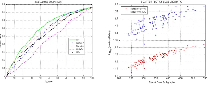
5.5. Embedding Comparison. Given a similarity measure like SN SCE, the choice of the embedding is critical for determining the quality of the retrieval results. Here, we consider the Commute Time (CT) embedding [39], Laplacian Eigenmaps (LEM) [5], Diffusion Maps (DM) [35], Heat Kernels (HK) [2], and ISOMAP [49] (in this latter case we use the shortest path lengths between nodes as geodesics) as alternative embeddings. The alternative embeddings rely on a function of the eigen-values (diagonal of Λ) and/or eigenvectors (columns of Φ) of a property matrix. For instance, HK and CT embeddings result from a functionF(.) applied to the Lapla-cianF(L) = ΦF(Λ)ΦT _{= Θ}T_{Θ, where the matrix of embedding co-ordinates Θ results} from the Young-Householder decomposition of the kernel. For CT,F(L) =√volΛ−1/2 while for HK we haveF(L) = exp −1

2tΛ

wheretis time. For DT we haveF(L) = Λt

3

where Λ results from a generalized eigenvalue/eigenvector problem as in the case of LEM where F(L) = Φ. Finally, ISOMAP considers the leading eigenvectors of the geodesic distance matrix. Different embeddings yield different point distributions for the same dimensionality. For instance, CT produces denser point clouds than LEM (see [39]). For structural retrieval with a distributional measure such asSN SCE, lo-cating the optimal function is critical, and must be determined empirically. Thus, we have obtained the retrieval-recall curves on the Gator database for each of the aforementioned embeddings with the settingd= 5. We plot the results in Fig. 9-Left. The CT embedding outperforms the alternatives. However, reasonable performance is obtained with ISOMAP and DM fort= 64 (a time setting that is sufficiently large to give an unfragmented embedding, given the size of the sub-sampled graphs).

Although CT gives good results, there are recent theoretical results which point to limitations of CT as a global characterization of kNN graphs for point-sets resulting from the denseness of the embedding (see for example the recent work of von Luxburg et al. [52][51]). More precisely, when we construct a kNN graph G over a large point-set, this implies a high edge density. Under these conditions, we have that the

resistence distance R(i, j) = CT_vol(₍i,j_G)) satisfies the condition R(i, j) ≈ _D(1i,i)+ 1

D(j,j).

In other words, it becomes meaningless as a measure of distance between vertices in a graph since it depends only on their degree and not their separating path length or edge weights. An experimental means of quantifying proximity to this limit is to analyze the ratio|R(i, j)−1/D(i, i)−1/D(j, j)|/R(i, j). If we plot the log(.) of the median of the ratio versus the size of the graphs, this should be monotonically decreasing with the size of the graphs. However, this is not the case for the Delaunay triangulation representations of graphs since the edge density is relatively low. In fact, for the Gator database the median of the edge densities is 0.3409(34%) and independent of graph size. In Fig. 9-Right we show that the ratio defined above is not decreasing. More importantly, the values of the ratio are even higher when

d= 5. This better performance for the five dimensional case is explained by the fact that dCT(i, j)≤CT(i, j), wheredCT(i, j) =||f(i)−f(j)||2 _{is the squared Euclidean}

distance between the d−dimensional embeddings of nodes i and j. This has the result of increasing the manifold density without loosing the global topology of the graph. This is not the case for the HK embedding which produces dense but poorly discriminating manifolds. Consequently it yields the poorest retrieval behavior.

5.6. The optimality of the CT embedding. In addition to the deviation of Delaunay triangulations from the von Luxburg law, we conjecture that the better behavior of the CT embedding derives from the reversibility of the embedding (that we explore in Section 6). In turn, such reversibility depends on the degree distribution of Delaunay triangulations, since node degree plays an important role in the CT embedding.

Let X ={x1,x2, . . . ,xn} be the points in Rn to be embedded into a subspace included inRd _{with d≪n, and} Wij = exp(−||xi−xj||2/σ2) the similarity matrix. Then, the CT embedding is given by the rows ofn×dmatrixZminimizing [39]

ǫ′=

Pn

i=1

Pd

j=1||Z(i)−Z(j)||2Wij

Pn

i=1

Pd

j=1ZijD(j, j)

=tr

_ZT_LZ

ZT_DZ

,

(5.1)

where L = D₋W is the Laplacian matrix and D is the diagonal degree matrix. Since the denominator of ǫ′ _{relies on the degrees, the optimal embedding can assign}

large coordinate values to nodes with large degree. This degree-of-freedom allows the scattering of embedded points so that the local structure of the original graph is preserved, because such local structure is determined by the degrees.

Recent studies [24] suggest that the degree distribution of Delaunay triangulations barely follows a power law. Following a power law means that few nodes have a large degree whereas most of them have small degrees. This produces an exponential decay of the sorted degrees and gives a linear behavior with negative slope in the log-log space. However, as we can see in Fig. 10, the slope of the decay is small (κ=−0.3) which means that the exponential decay is quite moderate. This increases the entropy of the degree distribution with respect to those with more pronounced decays. Then, since most of the nodes tend to have a moderate-high degree, the embedded points can be scattered according to their degrees. This maximizes the distances between the embedded points, at least globally. Since the numerator of Eq. 5.1 must be minimized, the CT embedding tends to map close points (or neighboring nodes, when adjacency matrices are considered instead of weight matrices) to the same cluster. However, the simultaneous minimization of the denominator tends to separate these clusters. In this way, the CT embedding amplifies the distance between tight groups.

This behavior in turn has an impact in entropy estimation since it relies on kNN tests. Nearest neighbors are frequently found in isolated clusters. It is well known that the curse of the dimensionality compromises the performance of kNN rules. However, when CT are used for embedding Delaunay triangulations entropy estimation is quite robust for highd, as this is the case with the Houses dataset.

Since the embedded nodes are not i.i.d., the bypass entropy estimator used in this paper tends to underestimate the Shannon entropy. The use of this estimator produces consistent results provided that we do not mix the graphs being compared, which is a relatively mild assumption in the computer vision domain.

are quite uniformly spaced, the embedding is prone to the curse of the dimensionality and then the kNN rules (and in turn the entropy estimator) fail.

As we will see in the next section, the combination of the properties of Delaunay triangulation and the nature of the CT embedding have a significant impact in the reversibility of the embedding.

0 1 2 3 4 5 6 7 8

x 104 2

4 6 8 10 12 14 16 18 20

Gator node

Degree

DEGREE DISTRIBUTION FOR GATOR NODES

Degrees of Gator Nodes

100 101

102 103

104 105 100

101 102

log(node)

log(Degree)

POWER LAW DISTRUTION OF GATOR DELAUNAYS

loglog(Degree) Linear fit

Fig. 10.Slight Power Law of degree distributions for Delaunay triangulations (Gator graphs). Left: degree distribution. Right: log-log curve and linear model fitting the data: slope isκ=−0.3.

6. From Distances to Structure. So far we have analyzed the CT embedding in itsdirectform. It provides a means of transforming the nodes of a graphG= (V, E) into points in ad−dimensional vector space. When d=|V|, then the Euclidean dis-tance between the point positions of pairs of nodes is equal to the commute time between them on the graph. When the embedding is into a subspace, i.e. d <|V|, then the Euclidean distance is upper bounded by the commute time. The embed-ding allows us to pose the problem of graph matching in terms of non-rigid point-set alignment (SEgm), and we then measure graph similarity through the SNSCE of the aligned samples. SNSCE is designed to compare twod-dimensional probability distri-butions, and implicitly this means that we are representing the graphs to be matched as multidimensional probability distributions. This interpretation opens up additional and intriguing novel perspectives. For instance,to what extent does the metric infor-mation in the embedding encode graph topology? One way of answering this question is to exploreto what extent metric information is preserved under the embedding and the extent to which it is reversible. In other words, under what conditions can we recover the original graph from its embedding? Moreover, if this is the case then can we use theinverseof a vectorial generative model for the distribution of points in the embedding space, as a means of sampling graphs? This is of pivotal importance for constucting generative models for graphs since state-of-the-art methods [23] are sub-ject to the combinatorial constraints associated with the original topological space. We conjecture that these constraints can be bypassed by constructing the prototype in a sub-space and then inverting the embedding.

In this section we propose an optimization algorithm (inverse embedding) to that end and also prove its convergence. Here we extend the formal results presented in [17].

graphG= (V, E) with|V| =N and adjacency matrixA. The problem of learning or inferring the graphGfrom the latter collection of multi-dimensional points can be posed as the following optimization problem

M ax X

j>i

Aij

s.t. Θij =||xi−xj||2

0≤Aij ≤1;∀i, j , (6.1)

where Θij=||Θ(i)−Θ(j)||2=CT(i, j) and Θ(i),Θ(j)are theN−dimensional coordi-nates of the embedded nodesiand j respectively. Following [39] we have

CT(i, j) =vol

N

X

z=2

1

λz

(φz(i)−φz(j))2, (6.2)

where vol is the volume of the graph and λz, φz denote z−th the eigenvalues and eigenvectors of the unknownnormalized LaplacianL. The embedding matrix is con-structed with

Θ =√volΛ−1/2ΦT ,

(6.3)

where Λ =diag(λ1= 0, λ2, . . . , λN) and Φ = [φ1φ2 . . . φN] is the matrix of eigenvec-tors which satisfies

||Θ(i)−Θ(j)||2=CT(i, j).

(6.4)

The maximization ofP_j>iAij is consistent with finding the closest graph to the complete one – the initial proposal – which satisfies all the embedding constraints.

Using Lagrange multipliers (one for each constraint) the problem is equivalent to maximizing Eq. 6.5 where the second (entropic) term relies on both axlog(x) barrier function and also depends onβ [41]. The third term contains theN(N−1)/2−N

Lagrange multipliersαij (one multiplier per constraint).

E(A,{αij}) =

X

ij:j>i

Aij+ 1

β

X

ij:j>i

Aij(logAij−1) + (6.5)

X

ij:j>i

αij(Θij− ||xi−xj||2)

.

The fixed point equations for updating theAij are given by

∂E ∂Aij

= 1 + 1

β logAij+αij ∂Θij

∂Aij

. ∂E

∂Aij

= 0⇒ _β1 logAij =−1−αij

∂Θij

∂Aij

⇒Aij = expβ

−1−αij

∂Θij

∂Aij

,

(6.6)

where ∂Θij

form solution and must be performed through gradient ascent, given the previously available estimates of the multipliers and distances:

∂E ∂αij

= Θij− ||xi−xj||2

⇒αtij+1=αtij+µ(Θtij− ||xi−xj||2), (6.7)

where µ ∈ [0,1] is the learning factor. In practice this factor must be set so that it decreases with the size of the graphs. The convergence of the inverse embedding procedure is dependant on the setting and control of this parameter.

6.2. Deterministic Annealing Algorithm. The fixed point equations for up-dating Aij and the gradient ascent equations designed for updating the multipliers

αij motivate the following deterministic annealing algorithm:

Initialize β=β0,Aij = 1/N, αij = 0, j > i, µ

Begin: Deterministic Annealing. Do whileβ≤βf

H ←ComposeAdjacencyM atrix({Aij}) Θ←Embedding(H)

αij←αij+µ(Θij− ||xi−xj||2) ∂Θij

∂Aij ←ComputeDerivative(i, j, A)

Aij ←expβ

−1−αij∂_∂AijΘij

β←ββr

End

G=M DLCleanup({αij})

In the algorithm above, the initializationAij = 1/N,∀i6=j, that is a barycenter depending on the complete graph (Aij = 1,∀i6=j), ensures that theN−dimensional points of the embedding matrix Θ are initially equally spaced. More precisely, in this case we have thatH= 1

NKN is the adjacency matrix of the uniformly weighted complete graph withN nodes, and the diagonal degree matrix isDH =N_N−1I. These two settings imply thatLH =I−_N1₋₁KN =LKN. Consequently, the commute times for both graphs (encoded byKN and _N1KN) are the same.

In a classic study on random walks [30] Lov´asz used a power series expansion to prove that in a complete graph of N nodes the hitting time between every pair of nodes isN −1. For this type of graph we therefore have that the hitting times are symmetric and henceCTH(i, j) = 2(N−1)∀i, j ∈VH. Lov´asz also derived universal lower and upper bounds for CT s for any type of graph. The bounds are given in Eq. 6.8 where λ2 is the Fiedler eigenvalue of the normalized Laplacian LG, that is, the so called spectral gap of G. Since for a complete graph we have λ2 = _NN₋₁, it

is straightforward to proof that CTH(i, j) = 2(N −1) where 2(N −1) is the upper bound. For any regular graph the lower bound is N. An in depth analysis by von Luxburg et al. [51] shows that the probability of obtaining an incorrect CT in a kNN graph tends to unity whenk/(logN)→ ∞, and this occurs when a single node is connected directly to the remainder. This type of structural pattern may appear in certain clustering problems, but does not arise for the types of graphs used in our target domain, i.e. computer vision. Here planar graphs are typically derived from region adjacency relations or are Delaunay triangulations of points.

upper bound appearing in Eq. (6.8), and this in turn means that large values of CT are admissible. For each graph in Gator we also show the distribution of the differences between CT and the quantity 2(N−1), whereNis the size of the corresponding graph. We observe that the difference is positive and varies approximately linearly with N. This suggests that most of the commute times between pairs of nodes are longer than the expected value for a complete graph of the same size. However, it is highly improbable that this is the case for immediately adjacent nodes. In Fig. 11-Right we distinguish between the commute times between immediately adjacent nodes and those between the remaining non-adjacent ones. As expected, the median values of

CT(i, j)−2(N−1)∀(i, j)∈Efor the adjacent nodes tend to be negative. However, the distribution of commute time is dominated byCT(i, j)∀(i, j)6∈E for the remaining nodes and this is why CT(i, j)−2(N−1)∀(i, j)6∈ E is both highly positive (≫0) and also increases with N.

vol(G) 2

1

D(i, i)+ 1

D(j, j)

≤CT(i, j)≤ vol_λ(G)

2

1

D(i, i)+ 1

D(j, j)

.

(6.8)

0 100 200 300 400 500 600 700 0

500 1000 1500 2000 2500

Size of GatorBait graphs SPECTRAL GAPS AND CTs−2*(N−1)

Spectral Gap x 10e+03 median(CT − 2*(N−1))

0 100 200 300 400 500 600 700 −1000

−500 0 500 1000 1500 2000 2500

Sizes of GatorBait graphs CTs−2*(N−1) FOR EDGES AND NOT−EDGES

(CT−2*(N−1)|Edge)*50 CT−2*(N−1)|NoEdge

Fig. 11.CT analysis of Gator. Left: CT-2(N-1) medians and spectral gaps(×103

for a better visualization). Right: CT-2(N-1) modes both for adjacent (×50) and non-adjacent nodes.

The analysis of CT above is key to understanding the dynamics of our inverse embedding method and how to initialize it. We commence with an initialization that ensures equal squared distances between embedded points, i.e. Θij = 2(N−1). More importantly we have Θij− ||xi−xj||2= Θij−CT(i, j) which is usually negative. In addition to the advantages of CT that we observe in Fig. 11, we have also provided a more principled argument for its use in Section 5.5. The moderate power law behavior of Delaunay triangulations in combination with the introduction of large distances between clusters in the CT motivates Θij−CT(i, j)<0 in many cases.

The deterministic annealing (DA) algorithm progresses by maximizing Eq. 6.5, which is dominated by the second term _β1P_ij:j>iAij(logAij−1) for low values ofβ. However, the elements of the adjacency matrixAij depend on the Lagrange multipliers

multipliers will be associated to edges of the recovered graph. In the Supplementary Material we detail the proof of convergence.

Once the algorithm has converged, we must extract the edges from the less nega-tive multipliers. We address this task using an MDL (Minimum Description Length) approach. We do not know in advance how many edges the hidden graph contains. We assume that it has a single connected component. Therefore, it seems reason-able to postprocess the multipliers so that we select the minimum number such that the resulting graph is connected. This procedure does not preclude us from using statistics regarding the number of edges, should these become available. We use the

blind inverse embedding, and sort the multipliers in ascending order according to their absolute value. We commence by selecting the firstk =N −1 multipliers to check whether we have found a connected graph ofN vertices (N−1 is the minimal number of edges that give a connected component on N vertices). If the multiplier

αij satisfies this condition then (i, j) is selected as an edge, i.e. Aij = 1 andAji= 1. If the condition is not satisfied we setAij =Aji= 0 to the not selected edges. If the resulting graph is not singly connected we makeA= 0 and repeat the latter procedure fork+ 1 until convergence to a single component (the number of connected compo-nents is detected using spectral graph theory). This part of the algorithm is called

M DLCleanup({αij}) and returns the MDL maximization of the objective function. The computational cost of the DA algorithm isO(N2_×N3_{) =O(N}5_{) since for each}

iteration we update a quadratic number of multipliers. Each update requires the com-putation of an embedding and thus the comcom-putation of eigenvalues and eigenvectors, which takesO(N3_{). However, as we will see in the experimental results for this part}

of the paper, for practical purposes the speed of convergence is very fast.

6.3. Results for Gator. We have successfully tested the proposed DA inverse-embedding on several types of graphs including linear ones. Linear graphs are difficult to obtain due to the fact that they are characterized by a small number of constraints (just (N −1) sufficiently large multipliers are required). In general, each type of graph requires a different value of the parameter µ (for example µ = 0.00001 for a linear graph ofN = 50 nodes andµ= 0.01 for a grid graph with 10×4 nodes each one with a maximum of 4 neighbors). In order to determine whether the required original (hidden) structure is recovered, we define an reconstruction error measure. We have usedE =Pij

|Aij−A∗

ij|

vol(G) whereGis the known graph (adjacency matrix) and

G∗ _{is the recovered adjacency matrix through inverse embedding. We consider both}

(i, j) and (j, i) as different edges, and thus we normalize by the volume of the graph. As a result E defines a relative error. For instance, the linear graph was recovered with zero error, whereas the grid-like graph was recovered withE= 0.3647 (36.47%). These preliminary results encouraged us to test our method on the challenging Gator database as a proof-of-concept of the usefulness of CT inverse embeddings to decode metric relations which are encoded by CTdirect embeddings.

In Fig. 12 we show the inverse embeddings of two example graphs of Gator (Fig. 12-Top-left). In both cases we setµ= 0.000000001 = 10−8_,β

0= 0.5,βr= 1.075

Fig. 12. Inverse embedding in Gator. Top-left: examples ofGator#1and Gator#5CT em-beddings for 3D (for visualization purposes since the complete dimensions are used in both cases). Top-right: evolution of the respective concave energy functions. Convergence speed is very fast. Bottom: comparison between the adjacency matrixAand the inferred graph A∗_{; in each image we} represent: 2A−A∗ _{so that coincident edges have value+1, edges inAbut not inA}∗ _{have value} +2and edges inA∗_{but not itGhave value−1. Most of the values are+1 with errors34.30%for}

Gator#1and39.53%forGator#2.

hypothesis and it is the underpinning mechanism for learning prototypical manifolds, and thus generative models, in the future.