fMRI Networks Using Integer Programming
.
White Rose Research Online URL for this paper:
http://eprints.whiterose.ac.uk/88737/
Version: Published Version
Article:
Costa, Lilia, Smith, Jim, Nichols, Thomas et al. (3 more authors) (2015) Searching
Multiregression Dynamic Models of Resting-State fMRI Networks Using Integer
Programming. Bayesian Analysis. pp. 441-478. ISSN 1931-6690
https://doi.org/10.1214/14-BA913
[email protected] https://eprints.whiterose.ac.uk/ Reuse
Items deposited in White Rose Research Online are protected by copyright, with all rights reserved unless indicated otherwise. They may be downloaded and/or printed for private study, or other acts as permitted by national copyright laws. The publisher or other rights holders may allow further reproduction and re-use of the full text version. This is indicated by the licence information on the White Rose Research Online record for the item.
Takedown
If you consider content in White Rose Research Online to be in breach of UK law, please notify us by
Searching Multiregression Dynamic Models of
Resting-State fMRI Networks Using Integer
Programming
Lilia Costa∗, Jim Smith†, Thomas Nichols‡, James Cussens§, Eugene P. Duff¶, and Tamar R. Makin
Abstract. A Multiregression Dynamic Model (MDM) is a class of multivariate time series that represents various dynamic causal processes in a graphical way. One of the advantages of this class is that, in contrast to many other Dynamic Bayesian Networks, the hypothesised relationships accommodate conditional con-jugate inference. We demonstrate for the first time how straightforward it is to search over all possible connectivity networks with dynamically changing inten-sity of transmission to find the Maximum a Posteriori Probability (MAP) model within this class. This search method is made feasible by using a novel applica-tion of an Integer Programming algorithm. The efficacy of applying this particular class of dynamic models to this domain is shown and more specifically the com-putational efficiency of a corresponding search of 11-node Directed Acyclic Graph (DAG) model space. We proceed to show how diagnostic methods, analogous to those defined for static Bayesian Networks, can be used to suggest embellishment of the model class to extend the process of model selection. All methods are il-lustrated using simulated and real resting-state functional Magnetic Resonance Imaging (fMRI) data.
Keywords:Multiregression Dynamic Model, Bayesian Network, Integer Program Algorithm, Model Selection, Functional magnetic resonance imaging (fMRI).
1
Introduction
In this paper a class of Dynamic Bayesian Network (DBN) models called the Multiregres-sion Dynamic Model (MDM) is applied to resting-state functional Magnetic Resonance Imaging (fMRI) data. Functional MRI consists of a dynamic acquisition, i.e. a series of images, which provides a time series at each volume element or voxel. These data are indirect measurements of blood flow, which in turn are related to neuronal activ-ity. A traditional fMRI experiment consists of alternating periods of active and control experimental conditions and the purpose is to compare brain activity between two dif-ferent cognitive states (e.g. remembering a list of words versus just passively reading a list of words). In contrast, a “resting-state” experiment is conducted by having the
∗The University of Warwick, UK; Universidade Federal da Bahia, BR, [email protected] †The University of Warwick, UK, [email protected]
‡The University of Warwick, UK, [email protected] §The University of York, UK, [email protected] ¶FMRIB Centre, Oxford University, UK, [email protected] FMRIB Centre, Oxford University, UK, [email protected]
c
subject remain in a state of quiet repose, and the analysis focuses on understanding the pattern of connectivity among different cerebral areas. The ultimate (and ambitious) goal is to understand how one neural system influences another (Poldrack et al.,2011). Some studies assume that the connection strengths between different brain regions are constant. Dynamic models have been proposed for resting-state fMRI, but they usually estimate the temporal correlation between brain regions (rather than the influence that one region exerts on another) or their scores are not a closed form which complicates the process of learning the network (seee.g.Chang and Glover,2010; Allen et al.,2014). However, clearly a more promising strategy would be to perform a search over a large class of models that is rich enough to capture the dynamic changes in the connectiv-ity strengths that are known to exist in this application. The Multiregression Dynamic Model (MDM) can do just this (Queen and Smith,1993; Queen and Albers,2009) and in this paper we demonstrate how it can be applied to resting fMRI.
To our knowledge, we present here the first application of Bayes factor MDM search. As with standard BNs, the Bayes factor of the MDM can be written in closed form, and thus the model space can be scored quickly. However, unlike a static BN that has been applied to this domain, the MDM modelsdynamic links and so allows us to discriminate between models that would be Markov equivalent in their static versions. Furthermore the directionality exhibited in the MDM graph can be associated with a causal directionality in a very natural way (Queen and Albers, 2009) which is also scientifically meaningful. Even for the moderate number of processes needed in this application the model space we need to search is very large; for example, a graph with just 6 nodes has over 87 million possible BNs, and for a 7 node graph there are over 58 billion (Steinsky,2003). Instead of considering approximate search strategies, we exploit recent technological advantages to perform a full search of the space, using a recent algorithm for searching graphical model spaces, the Integer Programming Algorithm (IPA; Cussens,2011). We are then able to demonstrate that the MDM-IPA is not only a useful method for detecting the existence of brain connectivity, but also for estimating its direction.
This paper also presents new prequential diagnostics customised to the needs of the MDM, analogous to those originally developed for static BNs, using the closed form of the one-step ahead predictive distribution (Cowell et al., 1999). These diagnostic methods are essential because it is well known that Bayes factor model selection methods can break down whenever no representative in the considered model class fits the data well. It is therefore extremely important to check that selected models are consistent with the observed series. We propose a strategy of using the MDM-IPA to initially search across a class of simple linear MDMs which are time homogeneous, linear and have no change points.
model and refine the analysis. Often, even after such embellishment, the model still stays within a conditionally conjugate class. Therefore if our diagnostics identify a serious deviation from the highest scoring simple MDM, we can adapt this model and its high scoring neighbours with features explaining the deviations. The model selection process using Bayes factors can then be reapplied to discover models that describe the process even better. In this way, we can iteratively augment the fitted model and its highest scoring competitors with embellishments until the search class accommodates the main features observed in the dynamic processes well. This is one advantage of adopting a fully Bayesian methodology to perform this analysis. Standard Bayesian diagnostics can be adapted to provide guidance in checking and where necessary to guide the modification of the model class.
The remainder of this paper is structured as follows. Section 2 provides a review of methods used to estimate connectivity and Section 3 shows the class of MDMs and a comparison between the MDM and these other methods. Section 4 then describes the MDM-IPA used to learn a network, and its performance is investigated using synthetic data. Section 5 gives diagnostic statistics for an MDM whilst its application to real fMRI data is shown in Section 6. Directions for future work are given in Section 7.
2
A Review of Some Methods for Discovering
Connectivity
Causal inference provides a set of statistical methods to allow us to tentatively move “from association to causation” (Pearl, 2009), or “from functional to effective con-nectivity” in neuroimaging terminology. In the study of functional integration, which considers how different parts of the brain work together to yield behaviour and cogni-tion, a distinction is made between functional connectivity and effective connectivity. The former is defined as correlation or statistical dependence among the measurements of neuronal activity of different areas, whilst the effective connectivity can be seen as a temporal dependence between brain areas and therefore it may be defined as dynamic (activity-dependent; Friston,2011).
A causal analysis is often represented using a directed graph where the tail of an arrow identifies a cause and the head its effect (seee.g.Figure1). Graphical models have been developed in order to define and discover putative causal links between variables (Lauritzen,1996; Pearl,2000; Spirtes et al.,2000). In this approach, the causal concepts are expressed in term of conditional independence among variables, expressed through a Bayesian Network (BN; see Section3), which are then extrapolated into a controlled domain (Korb and Nicholson, 2003). In such a graph, when there is a directed edge from one node to another, the former is called aparent while the latter is achild.
Figure 1: A graphical structure considering 4 nodes.
time point. For instance, Smith et al. (2011b) used a range of thresholds for each time series as 10th, 25th, 50th, 75th and 90th percentile. Patel et al. (2006) then calculated a measureκwhich compares the marginal probability that one region is active with condi-tional probability given that the other region is also active. In mathematical terms,κij
measures the distance betweenP(Y∗(i)|Y∗(j)) andP(Y∗(i)), and the distance between P(Y∗(j)|Y∗(i)) and P(Y∗(j)), whereY∗(i) is a dichotomized variable that represents
whether region i is active. This measure is found for each pair of brain areas. When
κij = 0, the conditional and marginal probabilities are the same and, in this sense, it
can be concluded that regionsiandj are not connected.
Finally, when two particular brain regions are connected (i.e.κij = 0), measureτij
is calculated based on the ratio of the marginal probabilities of each region, Y∗(i) and
Y∗(j). Whenτ
ij >0, the regioniis ascendant to the regionjwhilst the negative value
of this measure means that the regionjis ascendant to the former region. By definition, the node j is called ascendant to node i, if the marginal activation probability of the former node is larger than that of nodei.
There are many existing and useful alternate classes of model which investigate ef-fective connectivity. For instance a dynamic version of the BN is the Dynamic Bayesian Network (DBN), which takes account of the dynamic nature of a process, containing cer-tain hypotheses about the estimation of effective connectivity and embodies a particular type ofGranger causality (Granger,1969).
Granger causal hypotheses have recently been expressed in a state space form. Havlicek et al. (2010) developed a dynamic version of the multivariate autoregressive model, using a time-varying connectivity matrixAl(t). They write
Yt = L
l=1
Al(t)Yt−l+vt,
at = at−1+wt, wt∼ N(0,Wt),
where Lis the model order;Al(t) is then×nmatrix that represents the connectivity
between the past at lag l and the current observation variables, Yt, and n is the
zero-mean and varianceV whilstwtis innovation at timetwith the state varianceWt.
These dynamic autoregressive models allow cyclic dependences, but are very sensitive to the particular sampling rate. Also, model selection over the full model space is very complex because the dimension parameter space grows exponentially with maximal AR lag.
Classes like this one that directly model Granger causality have also received severe criticism when applied to the fMRI datasets (Chang et al., 2008; David et al., 2008; Vald´es-Sosa et al., 2011; Smith et al., 2012). In fact, Smith et al. (2011b) discovered that lag-based approaches like these do not perform well at identifying connections for fMRI data, albeit only under the assumption of static connectivity strength.
Other much more sophisticated classes of state space models have recently been developed to model effective connectivity. These include the Linear Dynamic System (LDS; Smith et al.,2010,2011a) and the Bilinear Dynamic System (BDS; Penny et al.,
2005; Ryali et al.,2011). Smith et al. (2011a) define the LDS as
Yt = βΦst/{t−L}+vt, vt∼ N(0,V);
st = Autst−1+Dutht+wt, wt∼ N(0,Wut);
where the observed fMRI signal (Yt) is written as a function of the parameterβthat
represents the weight of a known convolution matrix Φ, and the past at lag L of the latent variables, i.e.the quasi-neural level variables, st/{t−L} = (s′t−L, . . . ,s′t)′, being st= (st(1), . . . , st(n))′. The additive white Gaussian error is vt. The matrix Aut
rep-resents the relationships among the latent variables, and is therefore responsible for estimating the effective connectivities whilst the matrix Dut is the set of regression
coefficients of driving inputs (ht) on the latent variables; ut indexes the different
con-nectivity states over the duration of the experiment. In a BDS,Aut=A+BΛt, where
A indicates the interactions among latent variables without considering the influence of the experimental condition whilst the B represents the connections in the presence of modulatory inputs (Λt).
interaction was among observation or latent variables, or when the model included the convolution matrix or not.
Another popular approach in the neuroscience literature estimates effective connec-tivity using DCM (Friston et al., 2003; Stephan et al., 2008). The models are quite complex in structure and aim to capture specific scientific hypotheses. The determinis-tic DCM assumes that the latent variables are completely determined by the model,i.e.
the state variance is considered to be zero. As this version of DCM does not consider the influence of random fluctuation in neuronal activity, it cannot be used for resting-state connectivity (Penny et al.,2005; Smith et al.,2011a). More recently a stochastic DCM has been developed that addresses this problem (e.g. Daunizeau et al.,2009; Li et al.,
2011). Both versions of the DCM depend on a nonlinear biophysical “Balloon model”, making the inference process quite complex and unfeasible with more than but a few nodes (Stephan et al., 2010; Poldrack et al.,2011). Furthermore, several authors have criticised the use of the Balloon model as speculative (Roebroeck et al., 2011; Ryali et al., 2011), as there are alternate plausible models for the fMRI response.
Synchronization phenomena are also studied to investigate the communication be-tween different brain areas (Quian Quiroga et al., 2002; Pereda et al., 2005; Dauwels et al., 2010). Arnhold et al. (1999) proposed two non-linear measures to estimate the interdependence between two particular regions as
Sij =
1
T T
t=1
R(k)t (Y(i))
R(k)t (Y(i)|Y(j))
and
Hij = 1 T
T
t=1
log Rt(Y(i))
R(k)t (Y(i)|Y(j)) ,
whereT is the sample size,R(k)t (Y(i)) is the mean squared Euclidean distance to thek
nearest neighbours of the time series of region i,R(k)t (Y(i)|Y(j)) is the mean squared
Euclidean distance between Y(i) and the k nearest neighbours of the time series of regionj, and
Rt(Y(i)) = (1/T) T
t=1
R(Tt −1)(Y(i)).
In addition, Quian Quiroga et al. (2002) suggested a new measure as
Nij =
1
T T
t=1
Rt(Y(i))−Rt(k)(Y(i)|Y(j)) Rt(Y(i))
.
The measures Hij and Nij are more robust against noise than Sij, but the former is
not normalised whilst Nij is, assuming values between zero and one. Although these
A Linear Non-Gaussian Acyclic Model (LiNGAM) is used to estimate effective con-nectivity, based on the following assumptions: (1) data are generated through a linear process consistent with an acyclic graphical structure; (2) unobserved confounders are not allowed; (3) noise variables are mutually independent and have non-Gaussian distri-butions with non-zero variances (Shimizu et al.,2006). Thus supposeYis the observed data matrix. Then LiNGAM consists of the model:
Y=BY+e;
where Bis a lower triangular matrix with all zeros on the diagonal andeis a residual matrix. Solving forY,Y=Aeis obtained, whereA= (I−B)−1andIis the identity
matrix. The assumption of non-Gaussianity enables the direction of causality to be identified so that the effective connectivity can be estimated (Shimizu et al., 2006). Because the components ofemust be mutually independent and non-Gaussian,Acan be estimated in an identifiable way: Independent Component Analysis (ICA).
3
The Multiregression Dynamic Model
In this paper we propose a further class of models that can be applied to investigate effective connectivity. The MDM (Queen and Smith, 1993) is a graphical multivariate model for an n-dimensional time series Yt(1), . . . , Yt(n). This is a particular dynamic
generalisation of the family of Gaussian BNs, and we begin by describing this class.
The Bayesian Network (BN)
Bayesian Network models decompose the joint distribution of a set of observables into a set of conditional distributions. BNs embody the assumption of the Markov property, and only consider direct dependencies that are explicitly shown via edges (Korb and Nicholson, 2003). More explicitly, in a BN with nodes represented by the random variables Y = (Y(1), . . . , Y(n)), the chain rule allows the joint density to be factorized as the product of the distribution of the first node and transition distributions between the following nodes,i.e.:
py(y(1), y(2), . . . , y(n)) = p1(y(1))×p2(y(2)|y(1))
×. . .×pn(y(n)|y(1), . . . , y(n−1))
= p1(y(1))× n
r=2
pr(y(r)|y(1), . . . , y(r−1)).
Let P a(r) ⊆ {Y(1), . . . , Y(r−1)} and call P a(r) the parents of Y(r) — those nodes connected into Y(r) by a directed edge in the BN. The Markov properties depicted in the BN state that a node depends only on its parents. This allows us to simplify the expression above to
py(y(1), y(2), . . . , y(n)) =p1(y(1))× n
r=2
When observed variables are jointly Gaussian, the conditional distribution of variables is defined as (Y(r)|P a(r),θ(r), V(r))∼ N(P a(r)′θ(r), V(r)), where N(·,·) is a Gaussian distribution; in this context the regression coefficient θ(r) represents the functional connectivity strengths (except for the intercept); and r= 1, . . . , n.
A Description of the MDM
Now consider the column vector Y′t = (Yt(1), . . . , Yt(n)) which denotes the data
from n regions at time t. Denote their observed values designated respectively by yt′ = (yt(1), . . . , yt(n)). Let the time series until time t for region r = 1, . . . , n be Yt(r)′= (Y
1(r), . . . , Yt(r)). The MDM is defined bynobservation equations, a system
equation and initial information (Queen and Smith, 1993). The observation equations specify the time-varying regression parameters of each region on its parents. The sys-tem equation is a multivariate autoregressive model for the evolution of time-varying regression coefficients, and the initial information is given through a prior density for regression coefficients. Thus the multiregression dynamic model is specified in terms of a collection of conditional regression dynamic linear models (DLMs; West and Harrison,
1997), as follows:
We write theobservation equations as
Yt(r) =Ft(r)′θt(r) +vt(r), vt(r)∼ N(0, Vt(r));
where r = 1, . . . , n; t = 1, . . . , T; Ft(r)′ is a covariate vector with dimension pr
de-termined byP a(r); the first element of Ft(r)′ is 1, representing an intercept, and the
remaining columns are observed time series of its parents;pris the number of parents
of node r plus 1 (for the intercept). The pr-dimensional time-varying regression
coef-ficient θt(r) represents the effective connectivity (except for the intercept); andvt(r)
is the independent residual error with variance Vt(r). Concatenating the nregression
coefficients asθ′t = (θt(1)′, . . . ,θt(n)′) gives a vector of lengthp=nr=1pr. We next
write thesystem equation as
θt=Gtθt−1+wt, wt∼ N(0,Wt);
whereGt= blockdiag{Gt(1), . . . ,Gt(n)}, eachGt(r) being apr×prmatrix,wtare
in-novations for the latent regression coefficients, andWt= blockdiag{Wt(1), . . . ,Wt(n)},
eachWt(r) being apr×pr matrix. The errorwt is assumed independent ofvs for all t and s; vs = (vs(1), . . . , vs(n)). For most of the development we need only consider Gt(r) =Ipr, whereIpr is thepr-dimensional identity matrix. Because the errors follow
a Gaussian distribution and the relationship between the observed variables and their parents is linear, this class of model is called a linear MDM (LMDM; Queen et al.,2008). Notice that by settingWt=0andGtas the identity matrix we retrieve a Gaussian BN
as defined above, whose regression coefficients are given prior Gaussian distributions.
then the model equations are written as:
θt(r) = θt−1(r) +wt(r); wt(r)∼ N(0,Wt(r)) ;
Yt(1) = θt(1)(1) +vt(1);
Yt(2) = θt(1)(2) +vt(2);
Yt(3) = θt(1)(3) +θ (2)
t (3)Yt(1) +θ(3)t (3)Yt(2) +vt(3); Yt(4) = θt(1)(4) +θ
(2)
t (4)Yt(3) +vt(4); vt(r)∼ N(0, Vt(r)),
forr= 1, . . . ,4,p1= 1,p2= 1,p3= 3 andp4= 2. The effective connectivity strengths
of this example are thenθ(2)t (3), θ (3)
t (3) andθ (2) t (4).
Finally theinitial information is written as
(θ0|y0)∼ N(m0,C0);
where θ0 expresses the prior knowledge of the regression parameters, before observing
any data, given the information at timet= 0, i.e.y0. The mean vectorm0is an initial
estimate of the parameters and C0 is the p×p variance-covariance matrix. C0 can
be defined as blockdiag{C0(1), . . . ,C0(n)}, with eachC0(r) being apr square matrix.
When the observational variances are unknown and constant, i.e.Vt(r) =V(r) for all t, by definingφ(r) =V(r)−1, a prior
(φ(r)|y0)∼ G
n0(r)
2 ,
d0(r)
2
,
where G(·,·) denotes a Gamma distribution, leads to a conjugate analysis where con-ditionally each component of the marginal likelihood has a Student t distribution. In order to use this conjugate analysis it is convenient to reparameterise the model as Wt(r) = V(r)Wt∗(r) and C0(r) = V(r)C∗0(r). For a fixed innovation signal matrix W∗t(r) this change implies no loss of generality (West and Harrison,1997).
This reparametrization simplifies the analysis. In particular, it allows us to define the innovation signal matrix indirectly in terms of a single hyperparameter for each compo-nent DLM called a discount factor (West and Harrison,1997; Petris et al.,2009). For the particular model selection purposes we require here, this well tested and expedient simplification vastly reduces the dimensionality of the model class, whilst in practice it usually loses very little in the quality of fit. This well used technique expresses different values ofW∗t(r) in terms of the loss of information in the change ofθ(r) between times
t−1 andt. More precisely, for someδ(r)∈(0,1], the state error covariance matrix
W∗t(r) =1−δ(r)
δ(r) C
∗ t−1(r);
where Ct(r) =V(r)Ct∗(r) is the posterior variance ofθt(r). Note that whenδ(r) = 1, W∗t(r) = 0Ipr, there are no stochastic changes in the state vector.
estimate δ(r) simply by maximising this marginal likelihood, performing a direct one-dimensional optimisation over δ(r), analogous to that used in Heard et al. (2006) to complete the search algorithm. The selected component model is then the one with the discount factor giving the highest associated Bayes factor score, as we will see later.
The joint density over the vector of observations associated with any MDM series can be factorized into the product of the density of the first node and the (conditional) transition densities between the subsequent nodes (Queen and Smith,1993). Moreover, the conditional one-step forecast distribution can be written as (Yt(r)|yt−1, P a(r))∼ Tnt−1(r)(ft(r), Qt(r)), whereTnt(r)(·,·) is a noncentral t distribution withnt(r) degrees
of freedom and the parameters are easily found throughKalman filter recurrences (see
e.g. West and Harrison, 1997). The joint log predictive likelihood (LPL) can then be calculated as
LPL(m) =
n
r=1 T
t=1
logptr(yt(r)|yt−1, P a(r), m), (1)
wheremdenotes the current choice of model that determines the relationship between the n regions expressed graphically through the underlying graph. The most popular Bayesian scoring method, and the one we use here, is the Bayes factor measure (Jeffreys,
1998; West and Harrison, 1997). Strictly in this context this simply uses the LPL(m):
m1 is preferred tom2 ifLP L(m1)> LP L(m2).
An Overview of the LMDM
The LMDM is a composition of simpler univariate regression dynamic linear models (DLMs; West and Harrison, 1997), which can model smooth changes in the parents’ effect on a given node during the period of investigation. There are four features of this model class that are useful for this study.
1. Each LMDM is defined in part by a directed acyclic graph (DAG) whose vertices are observed fMRI series at a given time. In addition, its directed edges represent the existence of a dependence on those contemporaneous observations that are ex-plicitly included as regressors to the receiving variable. In our context, therefore, these directed edges denote the hypothesis that direct contemporaneous relation-ships might exist between a variable and its parent. The directionality of the edges can be interpreted as being ‘causal’ in a sense that is carefully argued in Queen and Albers (2009);
2. Any LMDM enables a conjugate analysis. In particular its marginal likelihood can be expressed as a product of multivariate Studentt distributions, as detailed above. Its closed form allows us to perform a fast model selection;
Smith,1993, for an example of this). The use of joint Gaussian distributions has been criticised in the study of fMRI data;
4. The class of LMDM can be further modified to include other features that might be necessary in a straightforward and convenient manner: for example by adding dependence on the past of the parents (not just the present), allowing for change points, and other embellishments that we illustrate below.
Comparison with Other Models Used to Analyse fMRI Experiments
The LMDM is a dynamic version of the Gaussian BN, where, unlike the latter, the LMDM allows the strength of connectivity to change over time. By explicitly modelling drift in the directed connection parameters, the LMDM is able to discriminate between models whose graphs are Markov equivalent. By definition, two network structures are said to be Markov equivalent when they correspond to the same assertions of condi-tional independence (Heckerman, 1998). As a result two models, indistinguishable as BN models, become distinct when generalised into LMDMs, see an example of this in Section 5. The dynamic version of the BN is the DBN. This uses a Vector Autoregres-sion (VAR) type time series sequentially rather than the state space employed in the LMDM which can also be used to represent certain Granger causal hypotheses.
In the previous literature, a sliding time window has been used to estimate the dy-namic correlation among brain regions (Chang and Glover, 2010; Allen et al., 2014; Leonardi et al., 2013). Some methods have investigated change points in sparse undi-rected graphs (Cribben et al., 2012), or in the global structure, consisting of global chain and V dependences among three networks (Zhang et al., 2014). In contrast to the LMDM, these methods study functional connectivity, and also use sophisticated but much more complex statistical computational algorithms rather than conditional conjugate analyses to perform inference.
Possibly the closest family of competitive models are the dynamic Granger causal models (Havlicek et al., 2010) described above. These use Kalman filtering to obtain the posterior distribution of effective connectivity. However, in general, the scores of these models are not factorable and are therefore much slower to search over. The other methods, such as LDS, BDS and DCM, we reviewed in Section 2, are more sophisticated but also far too complicated to effectively score quickly enough over a large model space. Consequently these are not good candidates for use in the initial exploratory search we have in mind here. An important difference between these methods and LMDM is that while the dynamic of connectivity is directly estimated in LMDM, most other models consider connectivity as static or estimate only the different strengths of connectivity when modelling a different experimental situation. We show in our analyses below that in practice these strengths seem to drift in time. Of course some authors discuss the possibility of a connectivity for each time point, ut = t, including another dynamic
system for the connectivity, i.e. At = At−1+wat, where wat ∼ N(0,Wa)
sampler scheme) and there are some extra assumptions they need to make,e.g.a fixed varianceWa, which are not assumed in LMDM. Therefore, to our knowledge, no other competitive class of models generates formally justifiable scores in a closed form, and simultaneously allows connectivity to change over time in this way.
Bhattacharya et al. (2006) proposed a similar model for LDS, but with the assump-tion that the observaassump-tional errors are temporally dependent. This simpler class can also be implemented as a DLM (and so as an LMDM), as shown by West and Harrison (1997, ch. 9). Another modification in the model assumption was suggested by Bhattacharya and Maitra (2011). These authors proposed the autoregressive model for effective con-nectivity asAt=ρAt−1+wat, whereρis a parameter to be estimated. So implicitly
here we are using a random walk model for effective connectivity,i.e.Gt=Ip. It would
be possible to use Gt =ρIp and a similar procedure provided by Petris et al. (2009,
ch. 4) to estimate the matrix Gwithin our method. However, this again gives rise to further complexities and certain computational issues.
Other models also need to use approximate inferential methods such as an Expec-tation Maximisation algorithm (EM) or Variational Bayes (VB) which are still quite difficult to implement for these classes and add other problems to the model selection process. They also often use a bootstrap analysis to verify if the effective connectivity is significant dramatically slowing down any search. Thus, searching over these classes becomes more difficult and time consuming: a particular problem is that here we are se-lecting from a large set of alternative hypotheses. So LMDM provides a very promising fast and informative explanatory data analysis of the nature of the dynamic network.
Another important advantage of the LMDM over most of its competitors is that it comes with a customised suite of diagnostic methods. We demonstrate some of these below.
4
Scoring the MDM Using an Integer Programming
Algorithm
It is well known that finding the highest scoring model even within the class of vanilla BNs is challenging. Even after using prior information to limit this number to scien-tifically plausible ones, it is usually necessary to use search algorithms to guide the selection. However recently there have been significant advances in performing this task (see e.g.Meek, 1997; Spirtes et al., 2000; Ramsey et al.,2010; Cussens, 2010; Cowell,
2013), and below we make use of one of the most powerful methods currently avail-able. We exploit the additive nature of the MDM score function — equation (1), where there are exactly n terms, one per region. Each region has 2n−1 possible
Bayesian formulation of the processes, it is also possible to adapt established predictive diagnostics to this domain to further examine the discrepancies associated with the fit of the best scoring model and adjust the family where necessary. How this can be done is explained in the following section, and the results of such an analysis are illustrated in Section6.
Model selection algorithms for probabilistic graphical models can be classified into two categories: theconstraint-based method and thesearch-and-score method. The for-mer uses the conditional independence constraints whilst the latter chooses a model structure that provides the best trade-off between fit to data and model complexity us-ing a scorus-ing metric. For instance, the PC (“Peter and Clark”) algorithm is a constraint-based method and searches for a partially directed acyclic graph (PDAG; Meek, 1995; Spirtes et al.,2000; Kalisch and B¨uhlmann, 2008). A PDAG is a graph that may have both undirected and directed edges but no cycles. This algorithm searches for a PDAG that represents a Markov equivalence class, beginning with a complete undirected graph. Then, edges are gradually deleted according to discovered conditional independence. This means that edges are firstly deleted if they link variables that are unconditionally independent. The same applies if the variables are independent conditional on one other variable, conditional on two other variables, and so on. In contrast, Greedy Equivalence Search (GES) is a search-and-score method using the Bayes Information Criterion (BIC; Schwarz et al.,1978) to score the candidate structures (Meek,1997; Chickering,2003). The algorithm starts with an empty graph, in which all nodes are independent and then gradually, all possible single-edges are compared and one is added each time. This process stops when the BIC score no longer improves. At this point, a reverse process is then driven in which edges are removed in the way described above. Again, when the improvement of the score is not possible, the graphical structure that represents a DAG equivalence class is chosen (Ramsey et al.,2010). Note that as PC and GES search for a Markov equivalence class, it is not possible to use them with MDM, which discriminates graphical structures that belong to the same equivalence class.
The Integer Programming Algorithm
The insight we use in this paper is that the problem of searching graphical structures for MDM can be seen as an optimization problem suitable for solving with an integer programming(IP) algorithm. Here, we use IP for the first time to search for the graphical structure for the MDM, adapting established IP methods used for BN learning. Cussens (2010) developed a search approach for the BN pedigree reconstruction with the help of auxiliary integer-valued variables, whilst Cowell (2013) used a dynamic programming approach with a greedy search setting for this same problem. Jaakkola et al. (2010) also applied IP, but instead of using auxiliary variables, they worked withcluster-based constraints as explained below. Cussens (2011) took a similar approach to Jaakkola et al. (2010) but with different search algorithms. The MDM-IP algorithm follows the approach provided by Cussens (2011), but with the MDM scores given by LPL rather than BN scores, as we will show below.
Student t distributions. By equation1, the joint log predictive likelihood can be written as the sum of the log predictive likelihood for each observation series given its parents: a modularity property (Heckerman, 1998). This assumption says that the predictive likelihood of a particular node depends on only the graphical structure, i.e., if the set of parents of nodeiinm1is the same as inm2, thenLP L(Y(i)|m1) =LP L(Y(i)|m2).
Therefore, for any candidate modelm, LPL(m) is a sum ofn‘local scores’, one for each node r, and the local score forYt(r) is determined by the choice of parent setP am(r)
specified by the modelm. Letc(r, P am(r))=Tt=1logptr(yt(r)|yt−1, P am(r)), the local
score, so that LPL(m) =n
r=1c(r, P am(r)).
Rather than viewing the model selection for the MDM directly as a search for a model
m, we view it as a search fornsubsetsP a(1), . . . P a(n) which maximisen
r=1c(r, P a(r))
subject to there existing an MDM modelm withP a(r) =P am(r) forr= 1, . . . n. We
thus choose to see model selection as a problem of constrained discrete optimisation. In the first step of our approach we compute local scoresc(r, P a) for all possible values of P a and r. Next we create indicator variables I(r ← P a), one for each local score.
I(r ← P a) = 1 indicates that P am(r) = P a in some candidate model m. Note that
creating all these local scores and variables is practical considering the number of nodes in this application. The model selection problem can now be posed in terms of the
I(r←P a) variables:
Choose values for theI(r←P a) variables to maximise
c(r, P a)I(r←P a) (2)
subject to there existing an MDM modelmwithI(r←P a) = 1 iffP a=P am(r).
We choose aninteger programming (IP)(Wolsey,1998) representation for this prob-lem. To be an IP problem the objective function must be linear, and all variables must take integer values. Both of these are indeed the case in this application. However, in addition, all constraints on solutions must be linear—an issue which we now consider.
Clearly, any model m determines exactly one parent set for each Yt(r). This is
represented by the followingnlinearconvexity constraints:
∀r= 1, . . . n:
P a
I(r←P a) = 1. (3)
It is not difficult to see that constraints (3) alone are enough to ensure that any solution to our IP problem represents a directed graph (digraph). Additional constraints are required to ensure that any such graph isacylic.
have at least one member with no parents in that subset. Formally:
∀C⊆ {1, . . . , n}:
r∈C
P a:P a∩C=∅
I(r←P a)≥1. (4)
Maximising the linear function (2) subject to linear constraints (3) and (4) is an IP problem. For values of n which are not large, such as those considered in the current paper, it is possible to explicitly represent all linear constraints. An off-the-shelf IP solver such as CPLEX (Cussens,2011) can then be used for model selection.
To solve our IP problem we have used theGOBNILPsystem (Cussens,2011; Bartlett
and Cussens,2013) which uses theSCIPIP framework (Achterberg,2007). InGOBNILP
the convexity constraints (3) are present initially but not the cluster constraints (4). As is typical in IP solving, GOBNILPfirst solves the linear relaxation of the IP where the
I(r←P a) variables are allowed to take any value in [0,1] not just 0 or 1. The linear relaxation can be solved very quickly. GOBNILP then searches for cluster constraints
which are violated by the solution to the linear relaxation. Any such cluster constraints are added to the IP (as so-calledcutting planes) and the linear relaxation of this new IP is then solved and cutting planes for this new linear relaxation are then sought, and so on. If at any point the solution to the linear relaxation represents an acylic digraph, the problem is solved. It may be the case that no cluster constraint cutting planes can be found, even though the problem has not been solved. In this case GOBNILP resorts to
branch-and-bound search. In all cases, we are able to solve the problem to optimality, returning an MDM model which is guaranteed to have maximal joint log predictive likelihood (LPL).
The Running Time of the MDM-IPA
The learning network process follows two steps. Initially, the scores for each set of parents for individual nodes are found. Then the MDM-IPA is applied to discover the best MDM over all nodes.
The run-time of the first step (finding the scores) of course depends critically on the number of nodes and the sample size. It is necessary to fit a linear dynamic model for every node and every set of parents — there are 2n−1possible sets of parents per node. In addition, when the observational variance is unknown, it is necessary to fit every model several times, according to different values of the discount factor (DF). Then the model (with a particular value of DF) which provides the highest score is selected.
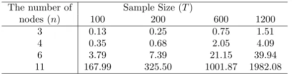
Table1shows the time taken in minutes to find the scores for different numbers of nodes and sample size, on a 2.7 GHz quad-core Intel Core i7 linux host with 16 GB, using the software R1. The discount factor was chosen in the range from 0.5 to 1.0 with
increments of 0.01. There is a sharp increase in the process time when the underlying graph has 11 or more nodes.
The application of the IPA to scores found in the first step is usually fast. For
The number of Sample Size (T)
nodes (n) 100 200 600 1200
3 0.13 0.25 0.75 1.51
4 0.35 0.68 2.05 4.09
6 3.79 7.39 21.15 39.94
[image:17.612.160.454.119.194.2]11 167.99 325.50 1001.87 1982.08
Table 1: The time in minutes to find the scores for different numbers of nodes and sample sizes, and the discount factor was chosen in the range from 0.5 to 1.0 with increments of 0.01.
11-node networks, the IPA took around 30 seconds using the softwareGOBNILP2.
An Application of the MDM-IPA Using a Synthetic fMRI Dataset
We now demonstrate the competitive performance of the MDM-IPA using a simu-lated fMRI time series data (Smith et al.,2011b). These data were generated using the DCM fMRI forward model and considering some of the characteristics that have been found in typical fMRI data analysed so far,e.g.set so that the amplitude of the neural time series is of a typical magnitude. Note that because the simulation was not driven by an MDM, we could not know a priori that this class of model would not necessarily fit this dataset well. It therefore provided a rigorous test of our methods within the suite of simulates available.
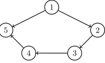
Here we chose the dataset sim22 from Smith et al. (2011b), which has 5 regions, 10min-session, time resolution (i.e.sample rate) of 3.00s, 50 replications and the same graphical structure (see Figure2). The connection strength was defined according to a random process and therefore varies over time, as Smith et al. explain: “The strength of connection between any two connected nodes is either unaffected, or reduced to zero, according to the state of a random external bistable process that is unique for that connection. The transition probabilities of this modulating input are set such that the mean duration of interrupted connections is around 30s, and the mean time of full connections is about 20s.”
The log predictive likelihood (LPL) was first computed for different values of discount factorδ, using a weakly informative prior withn0(r) =d0(r) = 0.001 andC∗0(r) = 3Ipr
for allr. The discount factors were chosen as the value that maximised the LPL, and so the average DF over all replications and nodes was around 0.85 (smaller than 1). Note that the MDM correctly identified that connectivities have been simulated to vary over time.
Smith et al. (2011b) compared different connectivity estimation methods ranging from the simplest approach which only considered pairwise relationships, such as cor-relation across the variables in the different time series, to complex approaches which
Figure 2: The graphical structure used by Smith et al. (2011b) to simulate data.
estimated a global network using all nodes simultaneously, such as BNs. The main mea-sures that they used to compare these methods werec-sensitivity andd-accuracy. The former represents the ability of the method to correctly detect the presence of the con-nection, while the latter shows the ability of methods to distinguish the directionality of the relation between the nodes.
The first measure calculated was c-sensitivity as a function of the estimated strength connectivity of the true positive (TP) edges which exist in both the true and the es-timated graph, regardless of the directionality, and the false positive (FP) edges that exist in the estimated graph but not in the true DAG. Here, we assess the performance of the methods in detecting the presence of a network connection, using the following measures:
• Sensitivity= #T P/(#T P+ #F N), where # represents “the number of” and FN is an abbreviation for false negative edge which is a true connection that does not appear in the estimated graph. This measure represents the proportion of true connections which are correctly estimated;
• Specificity = #T N/(#T N+ #F P), where TN is an abbreviation for a true neg-ative edge which does not exist in both true and estimated graphs: i.e.the pro-portion of connections which are correctly estimated as nonexistent;
• Positive Predictive Value= #T P/(#T P+#F P):i.e.the proportion of estimated connections which are in fact true;
• Negative Predictive Value= #T N/(#T N+ #F N):i.e.the proportion of connec-tions estimated as nonexistent that do not exist in the true graph;
• Success Rate = (#T P + #T N)/10, where 10 is the total number of possible connections for an undirected graph with 5 nodes. This represents the proportion of correctly estimated connections.
methods: the GES and the PC in the Tetrad IV1(see the definition of these methods in
the beginning of this section). The implementation of these methods is fairly easy, but unsurprisingly the computational time of the MDM is considerably higher than others because its descriptive search space is much larger. We estimated our sensitivity mea-sures, as described above, and Figure3(left) shows the average sensitivity measures over 50 replications for the MDM-IPA (blue bar), the GES (salmon bar) and the PC (green bar) methods. These approaches show satisfactory results for all measures, with the mean percentage above 75%. Although the PC has the highest percentage in Specificity and Positive Predictive Value, the MDM performs better in the three other measures. For instance, the MDM correctly detected around 90% of the true connections whilst PC and GES detected about 75% (sensitivity measure). Moreover, the MDM has the highest overall percentage of correct connections (success rate).
As a second method of comparison, Smith et al. (2011b) proposed a way to com-pare the performance of the methods in detecting the direction of connectivity. The d-accuracy is calculated as the percentage of directed edges that are detected correctly. This measure is given in Figure 3 (right). Again the MDM obtained some of the best results for this measure. Other methods that also had good results according to this criterion were Patel’s measures (Patel et al., 2006) and Generalised synchronization (Gen Synch; Quian Quiroga et al., 2002). We note that the performance of LiNGAM was poor when compared with other methods.
Although the d-accuracy of Patel’sτ and Gen Synch is not substantially different from that of the MDM (Figure3, right), these two former methods have only moderate c-sensitivity scores (Smith et al., 2011b). The opposite pattern can be seen for the methods based on the BN: they perform well in c-sensitivity but poorly in d-accuracy. Thus, only the MDM performed well in all the measures at the individual level of analysis.
An MDM Synthetic Study
We have showed the performance of the MDM-IPA considering synthetic data from 5-node networks. It would be interesting to see how this search algorithm performs with a larger number of nodes. However, although Smith et al. (2011b) provided higher dimensional DCM fMRI synthetic data, none of these were generated considering the stochastic process in connectivity strengths. We therefore generated the MDM data based on our analysis of the resting-state experiment studied in Section6. More specifi-cally, we fixed the 11 nodes and 230 time points in this experiment and simulated data of this size assuming as true the best fitting MDM model we found for the original data set (green edges in Figure 4). More details about the simulation process are described in Appendix A.
Figure 3: (left) The average over 50 replications of the sensitivity (Sens) = T P/(T P +
F N); specificity (Spec) = T N/(T N+F P); positive predictive value (PPV) = T P/(T P +
F P); negative predictive value (NPV) = T N/(T N +F N); (SR) success rate = (T P +
T N)/(total number of connections) for three methods: MDM (blue bar), GES (salmon bar) and PC (green bar). (right) The average over 50 replications of the percentage of directed connections that was detected correctly for some methods. The results of this second figure are from Smith et al. (2011b), except for the method MDM.
Figure 4: The graphical structure estimated for subject 7 using the MDM-IPA. The green edges are the significant connectivities found in the group analysis (see Figure7(b) in Section 6 below).
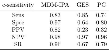
[image:20.612.209.403.387.570.2]5 nodes and the MDM with 11 nodes) have a similar variability of connections over time. When Smith et al. (2011b) compared the results of data over different numbers of nodes, they concluded that the classification order of methods considering c-sensitivity and d-accuracy measures is extremely similar for 5, 10, and 15 nodes. Here, considering the algorithms GES, PC and MDM-IPA, we came to the same conclusion. Table 2
shows that in general the MDM-IPA has the highest c-sensitivity measures and much better scores. While almost 80% of the estimated connections are actually true (PPV measure) for the MDM-IPA in both sets of synthetic data, for the GES this percentage was 85% in 5-node networks and it decreased to around 20% in 11-node networks (the PC provided a similar pattern). A plausible reason for this is that the number of false positive connections is dramatically higher for the GES and the PC than for the MDM-IPA in 11-node networks,i.e.the average #F P over replications for the GES, the PC and the MDM-IPA, respectively, was around 0.7, 0.4 and 1.0 in 5-node networks, and around 10, 18 and 2 in 11-node networks. Although the prevalence of FP increases with the number of nodes, their connectivity strengths usually are close to zero, as shown below.
c-sensitivity MDM-IPA GES PC
Sens 0.83 0.85 0.74
Spec 0.97 0.64 0.80
PPV 0.82 0.23 0.32
NPV 0.98 0.97 0.96
[image:21.612.216.395.325.407.2]SR 0.96 0.67 0.79
Table 2:The average over 50 replications of thesensitivity(Sens) =T P/(T P+F N);specificity
(Spec) =T N/(T N+F P);positive predictive value(PPV) =T P/(T P+F P);negative predictive value(NPV) =T N/(T N+F N); (SR)success rate= (T P+T N)/(total number of connections) for three methods: the MDM-IPA, the GES and the PC, considering 11-node networks synthetic data.
Regarding the d-accuracy criteria, the MDM-IPA also demonstrated greater power in detecting the direction of connectivity than the GES and the PC — 60%, 45% and 26% of directed edges were detected correctly in 11-node networks for the MDM-IPA, the GES and the PC, respectively.
In addition, we evaluated the proportion of timeP Trithat the true value of
connec-tionifor node ris inside the 95% smoothed highest posterior density (HPD) interval. As a result, the average of P Tri over all replications, considering only TP connections
(green edges in Figure4), was 96%, and therefore the MDM-IPA was shown to be effi-cient not only in detecting the edges, but also in estimating the connectivity strengths.
There are two kinds of FP connections: (situation 1) the edges exist in both the true and the estimated networks, but with opposite directions (e.g.connection 9→10 exists in the estimated graph whilst the true connection is 10 →9), and (situation 2) the edges exist only in the estimated network (e.g. connection 4 → 10). Considering the true value of these FP regression parameters as zero, the average P Tri over all
(situation 1) was about 30%. This is no surprise, when the opposite connection strength is higher than zero. In contrast, the average P Tri over all replications, considering
the FP connections that do not exist even on an undirected true network (situation 2) was 75%. This shows that when the MDM-IPA provides spurious connections, the associated connectivity strengths are usually close to zero. It is interesting to note that this appearance of spurious but weak dependences is a well known phenomenon when fitting more standard graphical models using Bayes factor methods. More robust conjugate Bayes model selection methods have recently been investigated using non-local priors (seee.g.Consonni and La Rocca,2011), and analyses of these could provide promising alternatives to the scoring methods in this paper.
5
The Use of Diagnostics in an MDM
In the past, Cowell et al. (1999) have convincingly argued that when fitting graphical models, it is extremely important to customise diagnostic methods, not only to deter-mine whether the model appears to be capturing the data generating mechanism well but also to suggest embellishments of the class that might fit better. Their preferred methods are based on a one step ahead prediction. We use these here. They give us a toolkit of sample methods for checking to see whether the best fitting model we have chosen through our selection methods is indeed broadly consistent with the data we have observed. We modified their statistics to give analogous diagnostics for use in our dynamic context. We give three types of diagnostic monitor, based on analogues for probabilistic networks (Cowell et al.,1999).
First theglobal monitor is used to compare networks. After identifying a DAG pro-viding the best explanation over the LMDM candidate models, the predicted relation-ship between a particular node and its parents can be explored through theparent-child monitor. Finally thenode monitor diagnostic can indicate whether the selected model fits adequately. If this is not so, then a more complex model will be substituted, as illustrated below.
I - Global Monitor
The first stage of our analysis is to select the best candidate DAG using simple LMDMs, as described in Section 4. It is well known that the prior distributions on the hyperparameters of candidate models sharing the same features must first be matched (Heckerman, 1998). In this way, the BF techniques can be successfully applied in the selection of non-stochastic graphs in real data. If this is not done, then one model can be preferred to another, not for structural reasons but for spurious ones. This is also true for the dynamic class of models we fit here.
likelihoods. We describe below how we have nevertheless matched priors to minimise this small effect in the consequent Bayes factor scores driving the model selection.
Just as for the BN to match priors, we can exploit a decomposition of the Bayes factor score for the MDMs. Because of the modularity property, when some features are incorporated within the model class, the relative score of such models only dis-criminates the components of the model where they differ. Thus, consider again the graphical structure in Figure1. For instance, suppose the LMDM is updated because node 3 exhibits heteroscedasticity. On observing this violation, the conditional one-step forecast distribution for node 3 can be replaced by one relating to a more com-plex model. Thus, a new one step ahead forecast density, p∗
t3(yt(3)|yt−1, yt(1), yt(2)),
is (Yt(3)|yt−1, yt(1), yt(2)) ∼ Tnt−1(3)(ft(3), Q
h
t(3)), where the parameters ft(3) and nt−1(3) are defined as before, but Qht(3) is now defined as a function of random
vari-ance, saykt3(Ft(3)′θt(3)) (see details in West and Harrison,1997, section 10.7). The
log Bayes factor comparing the original model with a heteroscedastic model is calculated as
log (BF) =
T
t=1
logpt3(yt(3)|yt−1, yt(1), yt(2))− T
t=1
logp∗t3(yt(3)|yt−1, yt(1), yt(2)).
We set prior densities over the same component parameters over different models, because the model structure is common for all other nodes. The BF then discriminates between two models by finding the one that best fits the dataonly from the component where they differ: in our example the component associated with node 3. Even in larger scale models like the ones we illustrate below, we can therefore make a simple modifi-cation of scores in order to use the IP algorithm derived above, and in this way adapt the scores over graphs almost instantaneously.
In this setting we have found that the distributions for hyperparameters of different candidate parent sets is not critical for the BF model selection, provided that early predictive densities are comparable. We have found that a very simple way of achiev-ing this is to set the prior covariance matrices over the regression parameters of each model a priori so that they are independent with a shared variance. Note the hyperpa-rameters and the parameterδ of the nodes 1, 2 and 4 were the same for both models: homoscedastic and heteroscedastic for node 3. Many numerical checks have convinced us that the results of the model selection we describe above are insensitive to these set-tingsprovidedthat the high scoring models pass various diagnostic tests some of which we discuss below.
An Application of the Global Monitor Using Synthetic Data
a simulation experiment. This in turn allows us to search over hypotheses expressing the potential deviations of causations.
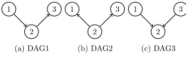
Here simulation of observations from known MDMs were studied using the graphical structure DAG1 (Figure5(a)), sample sizesT = 100, 200 and 300, and different dynamic levels W∗(r) = 0.001Ipr and 0.01Ipr. The impact of these different scenarios on the
[image:24.612.210.398.218.276.2]MDM results was verified regarding 3 regions and 100 datasets for eachT andW∗(r) pair. Details about the simulation process can be seen in Appendix B.
Figure 5: Directed acyclic graphs used in the MDM synthetic study. (a) DAG1 and (b) DAG2 are considered Markov equivalent whilst neither are equivalent to (c) DAG3.
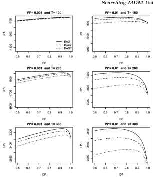
Figure6shows the log predictive likelihood versus different values of discount factor, considering DAG1 (solid lines), DAG2 (dashed lines) and DAG3 (dotted lines). The sample size increases from the first to the last row whilst the dynamic level (innovation variance) increases from the first to the last column. Although the ranges of the LPL differ across the graphs, the range sizes are the same, i.e. 500 so that it is easy to compare them.
An interesting result is that when data follow a dynamic system but are fitted by a static model, the non-Markov equivalent DAGs are distinguishable whilst equivalent DAGs are not. For instance, whenW∗(r) = 0.01Ipr andT = 100 (first row and second
column), the value of the LPL for DAG3 is smaller than the value for the other DAGs, but there is no significant difference between the values of the LPL for DAG1 and DAG2 when δ= 1, which we could deduce anyway since these models are Markov equivalent (seee.g.Ali et al.,2009). In contrast, there are important differences between the LPL of DAGs when dynamic data are fitted with dynamic models (δ <1), DAG1 having the largest LPL value. In particular, MDMs appear to select the appropriate direction of connectivity with a high success rate. However, their performance varies as a function of the innovation variance and sample size (note how the distance between the lines changes from one graph to another). For instance, as might be expected, the higher the sample size, the higher the chance of identifying the true DAG correctly. On the other hand,T has the greatest impact on the results when the dynamics of the data are very slowly changing (W∗(r) = 0.001Ipr). In this case the percentage of replications in which
the correct DAG was selected was 40%, 80% and 95%, for a sample size equal to 100, 200 and 300, respectively, whilst almost all the replications selected the DAG correctly for whicheverT andW∗(r) = 0.01Ipr.
II - Parent-child Monitor
Figure 6: The log predictive likelihood versus different values of discount factor (DF), for DAG1 (solid lines), DAG2 (dashed lines) and DAG3 (dotted lines). The sample size increases from the first to the last row whilst the dynamic level (innovation variance) increases from the first to the last column. The range of they−axis (LPL) is the same size: 500 for all graphs.
{Ypa(r)(1), . . . ,Ypa(r)(pr−1)}, then
log(BF)ri= logpr{y(r)|P a(r)} −logpri{y(r)|P a(r)\ypa(r)(i)},
for r = 1, . . . , n and i = 1, . . . , pr−1; where {P a(r)\Ypa(r)(i)} means the set of all
parents ofY(r) excluding the parent Ypa(r)(i).
III - Node Monitor
Again the modularity ensures that the model for any given node can be embellished based on residual analysis. For instance, consider a non-linear structure for a founder node r, i.e. one with no parents. On the basis of the partial autocorrelation of the residuals of the logarithm of the series, a more sophisticated model of the form
logYt(r) =θt(1)(r) +θ (2)
suggests itself. Note that this model still provides a closed form score for these compo-nents. The lower scores and their corresponding model estimation can then be substi-tuted for the original steady models to provide a much better scoring dynamic model, but they still respect the same causal structure as in the original analysis.
Denoting logYt(r) byZt(r), the conditional one-step forecast distribution forZt(r)
can then be calculated using a DLM on the transformed series {Zt}. More generally
if we hypothesize that Zt(r) can be written as a continuous and monotonic function
of Yt(r), sayg(.), and so the conditional one-step forecast cumulative distribution for Yt(r) can be found through
FYt(r)(y) = Ptr(Yt(r)≤y|y
t−1, P a(r))
= Ptr∗(Zt(r)≤g−1(y)|yt−1, P a(r))
= FZt(r)(g
−1(y)).
Thus p∗
tr(yt(r)|yt−1, P a(r)), the conditional one-step forecast density forYt(r) for
this new model can be calculated explicitly (see details in West and Harrison, 1997, section 10.6).
Recall that when the variance is unknown, the conditional forecast distribution is a noncentral t distribution with a location parameter, say ft(r), scale parameter, Qt(r), and degrees of freedom, nt−1(r). The one-step forecast errors are defined as et(r) = Yt(r)−ft(r) and the standardised conditional one-step forecast errors as et(r)/Qt(r)(1/2). The assumption underlying the DLM is that the standardised
condi-tional one-step forecast errors have an approximate Gaussian distribution, whennt−1(r)
is large, and they are serially independent with constant variance (West and Harrison,
1997; Durbin and Koopman, 2012). These assumptions can be checked by looking at some graphs, such as a QQ-plot, standardised residuals versus time, cumulative stan-dardised residuals versus time and the autocorrelation function (ACF) plot (Smith,
1985; Harrison and West,1991; Durbin and Koopman,2012; Anacleto et al.,2013).
6
The Analysis of Real Resting-state fMRI Data
Finally, we demonstrate how our methods can be applied to a recent experiment where the appropriate MDM needs more nodes than in our previous examples so that the IPA becomes essential. We applied the MDM-IPA network learning procedure to a resting-state fMRI dataset (described in detail in Duff et al., 2013). Data were acquired on 15 subjects, and each acquisition consists of 230 time points, sampled every 1.3 seconds, with 2x2x2 mm3voxels. The FSL software2was used for preprocessing, including head
motion correction, an automated artifact removal procedure (Salimi-Khorshidi et al.,
2014) and intersubject registration. We use 11 brain regions defined on 5motor and 6
visual regions. Motor nodes were selected based on activation patterns during a finger-tapping task. The nodes were located within the cerebellum, Putamen, Supplementary Motor Area (SMA), Precentral Gyrus and Postcentral Gyrus (nodes numbered from 1
to 5 respectively). The visual nodes were selected based on activation patterns during presentation of abstract shapes in motion in the central visual field. The visual nodes used are Visual Cortex V1, V2, V3, V4, V5 and task negative (regions in peripheral V1 found to decrease with task in a separate study; nodes numbered from 6 to 11 respectively). The observed time series are computed as the average of fMRI data over the voxels of each of these defined brain areas. We note that these data are not the output of an ICA, which may confound the interpretation of the results.
Here we modelled each subject using the MDM-IPA method, and then compared the graphs of the brain connectivities across individuals. Using a weakly informative prior, the scores of all possible sets of parents for every node were found. The MDM-IPA was then used to discover the optimal graphical structure to explain the data from each subject. We assessed the intersubject consistency of the resulting networks by the prevalence of directed edges and by verifying completely homogeneous connectivity over the network. More specifically, we estimatedpij, the probability that an edgei→j
exists, as the proportion ˆpij of subjects with this particular edge among the identified
regions. The statistic we used measured the extent to whichpij> π, whereπis the edge
occurrence rate under homogeneity, set equal to the average of ˆpij over the 90 possible
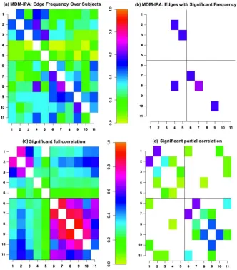
edges. Figure 7 (a) shows ˆpij for all connectivitiesi →j, where i indexes rows and j
columns. Figure7(b) also shows ˆpij, but only for those edges significant with a 5% false
discovery rate correction (FDR; Benjamini and Hochberg,1995). The black horizontal and vertical lines divide the figure into four squares; the top left square represents the connectivity between motor brain regions, whilst the lower right square represents the one between the visual brain regions. Unsurprisingly, most of connectivities are within these two squares. The two other squares represent cross-modalconnections, between motor and visual regions which are less prevalent.
We also consider two other methods of estimating the functional connectivity: full correlation andpartial correlation (Baba et al., 2004; Marrelec et al., 2006). For each subject, for each node pair, we computed the full and partial correlation, and thus Figure7(c) and (d) show the edges which appeared by chance with a probability higher than 0.95, respectively. Note that these techniques provide symmetric results about the principal diagonal. The vast majority of connections exist with high significance (Figure7 (c)), however, connections with the strongest correlation (above 0.6) tend to be intra-modal as discussed above. As expected, the significant MDM edges are a subset of the significant partial correlations (Figure 7 (d)). The nodes are ordered according to the expected flow of information in the brain, and thus it is notable that we find significant edges between consecutive nodes. In short, while full and partial correlations do not account for nonstationarities nor represent a particular joint model, Figure 7
demonstrates that the application of the MDM gives scientifically plausible results.
To illustrate the use of the parent-child monitor and node monitor, we selected subject 7 because its MDM-IPA result contains all edges that are significant in group analysis (Figure4), and so in this sense it was a typical experimental subject. Figure8
with other reports on the nonstationarities of resting-state fMRI (Allen et al., 2014; Ge et al.,2009; Leonardi et al., 2013) and demonstrates a key capability of this model. One possible explanation for the observed apparent changes in connectivity strengths proposed by Chang and Glover (2010) is that the level of attention, arousal and day-dreaming can differ during the resting-state experiment, and this is reflected through the measurements.
Figure 8: (Above) The smoothing posterior mean of connectivities (iny-axis) over time (in
x-axis).(Bottom)Discount factor for each node.
The group network (Figure 7 (b)) was fitted for all subjects and as a result the patterns shown in Figure8are consistent across subjects. For instance, the average DF for nodes that have parents was 0.96 for motor nodes and was 0.80 for visual nodes. It therefore appears that visual nodes have a shorter memory than motor nodes. A possible reason is that the physical/sensory environment is much more constrained/static than the visual environment. With this experiment, subjects were shown a screen with a fixation point. However, they were not explicitly asked to fixate. This might explain the greater perceptual variability in visual relative to sensory-motor areas.
Figure 9:The logBF at each time (dashed lines) and cumulative logBF (solid lines) comparing regions 2, 8, 9 and 10 as the set of parents of region 1 with the same set of parents but without region 8. The final logBF was 1.95 and therefore, there is evidence for the former model. This illustrates the use of the parent-child monitor.
log(BF)12 = logp1{y(1)|y(2),y(8),y(9),y(10)} −logp12{y(1)|y(2),y(9),y(10)},
which, as discussed above (Section 5), can be plotted over time. Figure 9 shows the individual contributions to the log(BF) as well as the cumulative log(BF). While the cumulative log(BF) is sometimes close to zero, there is a surge in evidence for the larger model (that includes 8 as a parent) near time point 110 and again after 180.
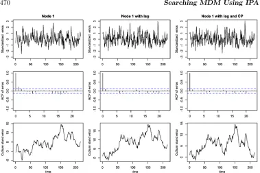
As discussed above, a simple LMDM can easily be embellished in order to solve problems detected by diagnostics measures. For example, Figure10(first column) shows the time series, ACF and cumulative sum plot of the standardised conditional one-step forecast errors for node 1. Note that the ACF-plot suggests autocorrelation at lag 1. This feature can still be modelled within the MDM class by making a local modification. For example, the past of region 1 may be included in its observation equation. That is,
Yt(1) = θ(1)t (1) +θ (2)
t (1)Yt(2) +θ(3)t (1)Yt(8) +θ(4)t (1)Yt(9) +θt(5)(1)Yt(10)
+θ(6)t (1)Yt−1(1) +vt(1).
Figure 10: Time series plot, ACF-plot and cumulative sum of one-step-ahead conditional forecast errors for region 1 (first column), consideringlag 1 (second column) and considering
lag 1 andchange points (third column). This illustrates the use of the node monitor.
particular threshold, a new model is fitted which entertains the possibility that a change point may have occurred.
Adopting this method and comparing the current graph with the graph where there is no parent from region 1, and with a threshold of 0.3, two time points were suggested as change points. It was straightforward to run a new MDM with a change point at the identified point, simply by increasing the state variance of the corresponding system error at these two points (West and Harrison, 1997, ch. 11). Figure 11 shows these two change points (dashed lines) and the filtering posterior mean for all connectivities for this region 1, considering both models, without (blue lines) and with (violet lines) change points. This gives us a different and higher scoring model, one whose score can still be calculated in closed form.
Note that although this naive approach seems to deal adequately with identified change points (see Figure10, third column), it can obviously be improved, for example by using the full power of switching state space models (see e.g.Fr¨uhwirth-Schnatter,
2006, ch. 13) to model this apparent phenomenon more formally, albeit with the loss of some simplicity. Normality and heteroscedasticity tests were also used in this study, but neither detected any significant deviation from the model class.