This is a repository copy of
Nonlinear multigrid methods for second order differential
operators with nonlinear diffusion coefficient
.
White Rose Research Online URL for this paper:
http://eprints.whiterose.ac.uk/82958/
Version: Accepted Version
Article:
Brabazon, KJ, Hubbard, ME and Jimack, PK (2014) Nonlinear multigrid methods for
second order differential operators with nonlinear diffusion coefficient. Computers and
Mathematics with Applications, 68 (12A). 1619 - 1634. ISSN 0898-1221
https://doi.org/10.1016/j.camwa.2014.11.002
[email protected] Reuse
Unless indicated otherwise, fulltext items are protected by copyright with all rights reserved. The copyright exception in section 29 of the Copyright, Designs and Patents Act 1988 allows the making of a single copy solely for the purpose of non-commercial research or private study within the limits of fair dealing. The publisher or other rights-holder may allow further reproduction and re-use of this version - refer to the White Rose Research Online record for this item. Where records identify the publisher as the copyright holder, users can verify any specific terms of use on the publisher’s website.
Takedown
If you consider content in White Rose Research Online to be in breach of UK law, please notify us by
Nonlinear Multigrid Methods for Second Order
Differential Operators with Nonlinear Diffusion
Coefficient
K.J. Brabazona,∗
, M.E. Hubbarda,b, P.K. Jimacka
a
School of Computing, University of Leeds, Leeds, LS2 9JT, UK
b
School of Mathematical Sciences, The University of Nottingham, University Park, Nottingham, NG7 2RD
Abstract
Nonlinear multigrid methods such as the Full Approximation Scheme (FAS) and Newton-multigrid (Newton-MG) are well established as fast solvers for nonlin-ear PDEs of elliptic and parabolic type. In this paper we consider Newton-MG and FAS iterations applied to second order differential operators with nonlinear diffusion coefficient. Under mild assumptions arising in practical applications, an approximation (shown to be sharp) of the execution time of the algorithms is derived, which demonstrates that Newton-MG can be expected to be a faster iteration than a standard FAS iteration for a finite element discretisation. Re-sults are provided for elliptic and parabolic problems, demonstrating a faster execution time as well as greater stability of the Newton-MG iteration. Results are explained using current theory for the convergence of multigrid methods, giving a qualitative insight into how the nonlinear multigrid methods can be expected to perform in practice.
Keywords: Nonlinear Multigrid, Newton’s Method, Nonlinear Diffusion 2010 MSC: 35J60, 35J92, 35K55
1. Introduction
Nonlinear multigrid iterations such as the Full Approximation Scheme (FAS) [9] and Newton-Multigrid (Newton-MG) [12, 48] methods have been widely used to solve elliptic and parabolic nonlinear problems on large scales (cf. [4, 17, 18, 21, 27, 42] amongst others). There exists very little convergence theory for the nonlinear methods (e.g. [2, 22, 25, 28]) and only limited com-parison as to which method should be preferred in practice [23, 26, 33, 34, 47],
∗Corresponding Author
Email addresses: [email protected](K.J. Brabazon),
[email protected](M.E. Hubbard),[email protected]
where the comparisons are limited to specific applications. In this paper we present a more general framework for comparing the relative efficiency of the Newton-MG and FAS methods for a broad class of nonlinear problems. This requires a detailed discussion of the efficient implementation of these schemes, followed by a theoretical assessment of their running times in a finite element setting for a general second order nonlinear operator. The comparison is based upon a detailed analysis of their costs per cycle, followed by a theoretical dis-cussion of their convergence properties and how this theory may be used when comparing the techniques. As there exists no algebraic variant of FAS multigrid, the geometric algorithms are compared.
The remainder of the paper is structured as follows. In section 2 we briefly present the linear and nonlinear multigrid iterations, followed by a detailed discussion of the theoretical running time of Newton-MG and FAS in section 3. Section 4 describes and applies the relevant convergence theory for linear and nonlinear multigrid iterations. In section 5 model problems are introduced, which are used to produce results in section 6, to demonstrate the applicability of the theory from sections 3 and 4. Conclusions are given in section 7, which summarise the reasons why a Newton-MG iteration should be preferred over an FAS iteration when using a finite element discretisation.
2. Background
In this section we introduce the basic concepts and notation required for the definition of both linear and nonlinear geometric multigrid algorithms. A more detailed introduction can be found in [12, 22, 48]. The problem to be solved is presented as an operator equation. Once an operator is discretised, and an appropriate basis for a discrete subspace has been chosen, the discrete operator equation may be considered an algebraic system of equations. In the following we move between considering operator equations and the corresponding alge-braic systems of equations, as appropriate.
2.1. Linear Multigrid Algorithms
We wish to solve the linear operator equation given by
Au(x) =f(x), x∈Ω (2.1) where the domain Ω∈ Rd has boundary ∂Ω, and A :V → V for some vector space V. From this point on we omit the explicit dependence on x ∈ Rd. It
is assumed that there is a unique u∗
∈ V satisfying equation (2.1). We are interested in the approximate solution of (2.1) based upon discretisations using a sequence of finite-dimensional grids
Ω1⊂Ω2⊂. . .⊂ΩJ, (2.2)
which are sets of connected points in Ω. We also consider the sequence of finite-dimensional function spaces
where eachVl,l = 1, . . . , J is defined on grid Ωl. Given (2.3), we consider the
discretised system of equations
Alul=fl (2.4)
where Al : Vl → Vl is the projection of the continuous operator A onto the
finite-dimensional spaceVl. We assume there are uniqueu∗l ∈Vl, l = 1, . . . , J
that satisfy (2.4). For the purposes of this paperVl,l= 1, . . . , Jis the standard
piecewise linear finite element function space defined on grid Ωl.
2.1.1. Linear Multigrid as a Solver
In this section we describe the linear geometric multigrid method and in-troduce some notation. A discussion of necessary conditions for convergence of geometric multigrid is presented in section 4.
We introduce operators
Rl:Vl→Vl−1, l= 2, . . . , J Pl:Vl−1→Vl, l= 2, . . . , J,
(2.5) which are restriction and prolongation operators, respectively, that allow the transfer of functions between different subspaces. Since the exact solution to (2.4) isu∗
l ∈Vl, the erroreland defectrlin approximationul, defined by
el=u∗l −ul, rl=fl−Alul,
satisfy the operator equation
Alel=rl. (2.6)
We assume there exist operators Sl : Vl →Vl, l = 2, . . . , J, called smoothing
operators, that have the property that they are effective at removing high fre-quency components from the error [12, 48]. A correction term is calculated on a coarser grid in thecoarse grid correctionstep. We fix a numberνof smooths to perform before (pre-smoothing) and after (post-smoothing) a coarse grid cor-rection step. In general the number of pre- and post-smooths may differ, and one of the smoothing steps may be left out entirely [12, 22, 48].
Consider that we wish to solve (2.4) on grid Ωl,l6= 1, for the exact discrete
solution u∗
l ∈ Vl. A single step of the geometric multigrid algorithm is then
outlined in algorithm 2.1, whereu(lj) ∈Vl represents the approximation to the
solutionu∗
l afterjiterations of linear multigrid have been performed. This
iter-ation can be performed until some appropriate convergence / failure criteria are met. On the coarsest grid level the exact inverse is very inexpensive to compute, provided that|Ω1| is small, and the running time of the algorithm isO(n) for
particular choices ofA (cf. [12, 48]). There is a closed form representation of the linear multigrid V-cycle operator, which for the rest of this paper is denoted
Ml :Vl→Vl. The exact representation can be found in [48]. A multigrid
Algorithm 2.1Multigrid V-Cycle
Require: Al, Al−1, Sl, Pl, Rl
1: functionLinear-MG(l, u(j)
l , fl, ν)
2: Setu′
l=Slνu
(j)
l
3: if l= 2thenCalculate ˜el−1=Al−−11Rl(fl−Alu′l)
4: else Set ˜el−1=Linear-MG(l−1,0, Rl(fl−Alu′l), ν)
returnu(lj+1)=Sν l(u
(j)
l +Ple˜l−1)
2.1.2. Multigrid Preconditioned Linear Iterations
Multigrid iterations are frequently used as a preconditioner for a different iterative method. For a more thorough discussion of such methods see [43]. The discrete problem (2.4) can be solved iteratively using a right-preconditioned Krylov subspace method, such as conjugate gradients (CG) or GMRES [43]. As the preconditioner we use a single multigrid V-cycle such that we solve
AlMlvl=fl, Ml−1ul=vl. (2.7)
Multigrid V-cycles used as a preconditioner for a Krylov subspace solver have been shown to be optimal in many situations (e.g. [13, 16, 49]).
2.2. Nonlinear Multigrid Algorithms
In this section we introduce nonlinear multigrid methods, using concepts introduced for linear multigrid methods.
2.2.1. Newton-Multigrid (Newton-MG)
An inexact Newton method is presented, which is given in detail in [14]. Consider the discrete nonlinear system
FJ(uJ(x)) = 0, (2.8)
for nonlinear operator FJ : VJ → VJ. ΩJ and VJ are the finest grid, and
associated subspace, in the hierarchies (2.2) and (2.3), respectively. Assume there exists a solutionu∗
J to (2.8) and that this is unique in
Bu∗
J ≡ {uJ ∈VJ :||uJ−u
∗
J||VJ < δ},
for someδ > 0. LetFJ be Fr`echet differentiable [38] in Bu∗
J and assume that
this derivative is invertible. A single step of an inexact Newton method is then given by algorithm 2.2.
Algorithm 2.2. Inexact Newton
uJ(j+1)=uJ(j)−AuJFJ(u
(j)
In algorithm 2.2 u(Jj) is the approximation after j inexact Newton iterations, and AuJ is some approximation to the inverse of the Fr´echet derivative ofFJ
(i.e. AuJ ≈F
′
J(u
(j)
J )
−1). The definition of A
uJ is required, which may be any
linear operator that approximates the inverse of the derivative of FJ at u
(j)
J .
LettingAuJ be a number of iterations of the linear multigrid operatorMJ (i.e.
AuJ =M
p
J for some (p∈N)>0) applied to the equationF
′
J(u
(j)
J )eJ =FJ(u
(j)
J )
gives a Newton-Multigrid (Newton-MG) iteration. We may use other choices forAuJ, including iterative Krylov subspace methods, and their preconditioned
variants, as described in section 2.1. 2.2.2. Full Approximation Scheme (FAS)
Brandt [9] was one of the first to introduce nonlinear multigrid, which seeks to use concepts from the linear multigrid iteration and apply them directly in the nonlinear setting. The iteration devised in [9] is called the Full Approximation Scheme (FAS) and it is this version of nonlinear multigrid that is considered in this paper. The Nonlinear Multilevel Method (NMLM) of Hackbusch [22] is a generalisation of FAS, but adds extra parameters into the algorithm. For brevity of discussion we consider only the FAS algorithm here, but note that the NMLM is a globally convergent iteration [25, 40]. Consider the discrete nonlinear problem
Al(ul) =fl, l= 1, . . . , J, (2.9)
with exact solution u∗
l unique in some Bu∗
l. This is equivalent to (2.8) with
Fl(ul) =Al(ul)−fl. The defect equation reads
Al(u∗l) =rl+Al(ul), (2.10)
where the defectrl=Al(ul∗)−Al(ul). As in the linear case, FAS is a
combina-tion of smoothing and coarse grid correccombina-tion. The smoothing operatorsSl are
nonlinear, but should possess the smoothing property, as in the linear case [22]. There are nonlinear variants of standard Jacobi and Gauss-Seidel smoothers, including variants to perform block smoothing (cf. [9, 12, 22, 48]). Using the prolongation and restriction operators given in (2.5), the nonlinear V-Cycle is defined in algorithm 2.3.
Algorithm 2.3FAS Multigrid
Require: Al, Al−1, Sl, Pl, Rl
1: functionFAS(l, u(j)
l , fl, ν)
2: Setu′
l=Slν(u
(j)
l )
3: Setu′l−1=Rlu′l ;fl−1=Rl(fl−Al(u′l)) +Al−1(u′l−1)
4: if l= 2thenCalculate ˜ul−1=A−1l−1(fl−1)
5: else Set ˜ul−1=FAS(l−1, u′l−1, fl−1, ν)
returnu(lj+1)=Sν l(u
′
l+Pl(˜ul−1−u′l−1))
of the error in the approximation. If the operators are linear then algorithm 2.3 is algebraically equivalent to algorithm 2.1 and hence is a generalisation of geometric multigrid to the nonlinear setting.
3. Computational Cost of FAS versus Newton-MG
There are several papers in which FAS multigrid is compared against Newton-MG for particular model problems [23, 33–35, 47]. Most of these compare the running times as well as the convergence factors, and come to the same con-clusion - that the execution time for Newton-MG methods is less than for FAS multigrid [33–35, 47]. For a finite difference discretisation the running times of the algorithms are shown to be much closer [26]. For finite differences the calcu-lation of the nonlinear residual is cheaper than for finite elements, as integrals over elements do not have to be calculated. The framework developed here can be used to show that this means that the execution time of an FAS iteration, relative to a Newton-MG iteration, will be less than for finite elements. For brevity this is not discussed in this paper.
In this section we consider the Newton-MG and FAS iterations applied to a general nonlinear problem. A theoretical bound on the running time is de-veloped that allows a direct comparison between the two methods and makes it clear why Newton-MG methods perform faster than FAS multigrid methods. In section 6 the sharpness of these bounds is demonstrated for model problems introduced in section 5. A note to make is that [23] finds that the Nonlinear Multilevel Method (NMLM) [22] performs better than a standard Newton-MG iteration. This is to be expected, though, as NMLM is a global algorithm. The same advantages of using Newton-MG over FAS can be found when compar-ing a global version of Newton’s method to the NMLM iteration, although this comparison is not presented in this paper.
We characterise the amount of computational effort required to perform each of the algorithms in terms of awork unit. One work unit (denoted Wl) is the
amount of time required to calculate the nonlinear residual on grid Ωl. The
amount of work required depends on the number of dimensions in which we are working, as well as the discretisation and choice of smoothers. In this section we present a general formula for calculating the amount of computational time required for a single linear or nonlinear V-cycle when using a finite element discretisation with piecewise linear basis functions on simplexes in arbitrary dimension. We then take an illustrative example to demonstrate the sharpness of the estimates.
We consider that we are working with the grid hierarchy described in (2.2), where Ωl⊂Rd, l = 1, . . . , J. We consider a linear finite element discretisation
with nodal basis functions such that span{ϕl i}
Nl
i=1=Vl,l= 1, . . . , J on a
quasi-regular simplicial partitioningTl(i.e. a triangulation in two dimensions, and a
partitioning into tetrahedra in three dimensions) on grid Ωl. The superscriptl
for the basis functions is dropped when it is apparent from the context which grid is referred to. Nl is the number of unknowns on grid Ωl. A fine grid simplicial
simplicial partitioning in one, two or three dimensions, respectively. In two dimensions and example of a quadrisection method is gained by connecting the mid-points of the edges of the elements. Hence, ifNlrepresents the number of
unknowns on grid Ωl, the number of unknowns on the next finest grid Ωl+1 is
given by
Nl+1≈2dNl. (3.1)
We consider that a problem has been given in weak form as
F(u, ϕ) = 0, ∀ϕ∈ V (3.2) and solve the discrete weak form given by
Fl(ul, ϕi) = 0, i= 1, . . . , Nl, (3.3)
for l = 1, . . . , J. The application of Fl can be calculated as a sum over the
elementsK ∈ Tlas follows:
Fl(ul, ϕi) =
X
K∈supp(ϕi)
Fl(K)(ul, ϕi), (3.4)
whereFl(K)is the discrete operator restricted to elementK ∈ Tl. Let the Fr`echet
derivative ofF(u, ϕ) atube denoted by
Fu(ψ, ϕ) =D[F(u, ϕ)] (ψ) (3.5)
and assume that this exists and is invertible for allu∈ V. Then the Jacobian matrix
h
Fu,l(ϕj, ϕi)
iNl
i,j=1 (3.6)
exists and is invertible, where Fu,l(·,·) is the discretisation of the Fr`echet
derivative on grid Ωl. For practical purposes we assume that the entries in the
Jacobian matrix are calculated using numerical differentiation, as for complex problems this requires less computational time to calculate than using exact formulas for the derivative. The entry in rowi, columnjof the Jacobian matrix is constructed as follows:
Fu,l(ϕj, ϕi)≈
X
K∈supp(ϕi)∩supp(ϕj)
Fl(K)(ul+ǫϕj, ϕi)−F(
K)
l (ul, ϕi)
ǫ . (3.7)
The valueFl(K)(ul, ϕi) is used in the calculation of the nonlinear residual, and
cost of calculating the Jacobian matrix and the residual is (d+ 2)Wl, whereWl
is the cost of calculating the residual on grid Ωl. Using similar reasoning we see
that calculating the diagonal entries of the Jacobian matrix requires an extra local function evaluation per node on each element. Hence the cost to calculate the nonlinear residual and the diagonals of the Jacobian matrix is 2Wl. The
diagonals of the Jacobian matrix are used in the nonlinear smoothing operator. We finally note that using (3.1) we can characterise the cost of calculating the nonlinear residual on grid Ωl−1 as
Wl−1≈
1
2dWl. (3.8)
LetCNMG(l) be the cost of performing a single Newton iteration on grid Ωl, and
CFAS(l) the cost of performing a single FAS V-cycle. From algorithms 2.2 and 2.3 we see that
CNMG(l) ≈CRJ(l)+
l−1 X
i=1
CJ(i)+pCLMG(l) (3.9)
CFAS(l) ≈CS(l)(ν1+ν2) +CRHS(l) +C (l−1)
FAS (3.10)
for CRJ(l) the cost of calculating the nonlinear residual and Jacobian; CJ(l) the cost of calculating the Jacobian; p the number of linear V-cycles to perform per Newton iteration; CLMG(l) the cost of performing a linear V-cycle; CS(l) the cost of a nonlinear smoothing operation; ν1 and ν2 the number of pre- and
post-smoothing iterations, respectively; and CRHS(l) the cost of calculating the perturbed right-hand side for FAS. In the characterisations (3.9) and (3.10) we have made the assumption that the nonlinear operations dominate the execution time of the two iterations, except for the inclusion of the linear multigrid cycle. As will be seen this is a fair assumption for the simple model problems presented, and becomes more accurate the more complicated the nonlinear operator is.
In (3.9) we see that the cost of the Newton iteration is given as the cost of calculating the residual and Jacobian matrix on the current grid level plus the cost of performing the linear multigrid iterations. We also include the calculation of the Jacobian matrix on the coarser grid levels here. This is because the results presented are for when the linearisation of the nonlinear operator is re-discretised on each grid level. We may instead use a Galerkin coarse grid operator (cf. [12, 48]), in which case the cost of interpolating the fine grid operator onto coarser grids should replace the cost of re-discretising the Jacobian on each grid level.
In (3.10) we see that the cost of the FAS iteration is given as the cost of smoothing on the current grid, calculating the perturbed right-hand side for the next coarsest grid, and performing an FAS V-cycle on the next coarsest grid. From previous discussion we have that
To calculate the cost of the nonlinear smoother we need to know which nonlinear smoother we are using. Assuming that we are performing a pointwise nonlinear smooth, such as nonlinear Jacobi (cf. [38]) we have to calculate the nonlinear residual in each iteration, as well as the diagonals of the current Jacobian matrix. Using previous discussion the cost of this is
CS(l)= 2Wl. (3.12)
This cost is accurate if we are performing a pointwise nonlinear Jacobi iteration. A pointwise Gauss-Seidel iteration requires the recalculation of the operator over the support of a basis function every time that a pointwise value is updated [47]. Hence a full pointwise nonlinear Gauss-Seidel iteration is considerably more expensive than the Jacobi iteration. If some block smooth is performed we need to calculate at least some off-diagonal entries in the Jacobian matrix. This means that the cost of a block smooth will also be considerably higher than the cost of the pointwise Jacobi smoother. In this investigation we consider the case of a Jacobi smoother, as this gives the smallest cost per iteration. Note that it is possible that a novel nonlinear smoother may be developed which is more efficient, or has much improved convergence properties, compared to a pointwise Jacobi iteration. Then FAS may become more competitive. However, it is highly unlikely that a novel smoother will give a large increase in performance, as when dealing with a nonlinear operator the nonlinear residual must be re-calculated in each smoothing step.
Finally we need to find the cost of calculating the perturbed right-hand side for the next coarsest grid level. From algorithm 2.3 we see that to calculate the perturbed right-hand side we calculate the residual on the current grid level, and apply the nonlinear operator to the restricted approximation on the coarser grid. The cost of applying the nonlinear operator is approximately the cost of calculating the residual on a given grid. Hence we have that
CRHS(l) =Wl+Wl−1= (1 + 2−d)Wl. (3.13)
We can now characterise the cost of both of the nonlinear iterations. We first consider Newton-MG, leaving the characterisation of the running time of the linear multigrid iteration until later. We find that
CNMG(l) = (d+ 2)Wl+ l−1 X
i=0
(d+ 2)Wi+pC
(l) LMG
= (d+ 2)
l
X
i=1
1
2idWl+pC
(l) LMG
≤(d+ 2) 2
d
2d−1Wl+pC
(l) LMG.
(3.14)
We are interested in knowing the running time per linear V-cycle, so we intro-duce a scaled variable
˜
CNMG(l) ≡C
(l) NMG
to be the cost per linear V-cycle of the Newton-MG algorithm.
Now consider the FAS multigrid iteration. We can approximate the cost of a single nonlinear V-cycle using the previous discussions as
CFAS(l) = 2Wl(ν1+ν2) + (1 + 2−d)Wl+C(l
−1) FAS
= ¡
2(ν1+ν2) + 1 + 2−d ¢
Wl+C(l
−1) FAS
= ¡
2(ν1+ν2) + 1 + 2−d¢ µ
Wl+
Wl
2d
¶
+CFAS(l−2)
= · · ·
= ¡
2(ν1+ν2) + 1 + 2−d¢ Ãl−1
X
i=1 Wl
2d(i−1) !
+CFAS(1)
≤ ¡
2(ν1+ν2) + 1 + 2−d¢
2d
2d−1Wl,
(3.16)
where in the last step we have assumed that the time taken to solve on the coarsest grid levelCFAS(1) is negligible compared toWl. This is usually the case,
but requires that the solution of the nonlinear equation is well approximated on the coarsest grid. If this is not the case then higher dimensional coarse spaces are required and the cost of the coarsest grid solve starts to have an adverse effect on the execution time.
We now compare the cost of a single nonlinear V-cycle to the cost of a linear V-cycle for a more specific problem. We restrict ourselves tod= 2 and estimate the running time of the linear multigrid algorithm in terms of a work unit. From empirical experiment we have found that an upper limit for a single V-cycle is given by
CLMG(l) ≤ 3
2Wl, (3.17)
where three linear pre- and post-smooths are performed. This ratio is a very good estimate for a simple model problem (cf. discussion of the p-Laplacian in section 5), and becomes more and more pessimistic as the complexity of the nonlinear operator increases. As the complexity of the nonlinear operator increases the cost of a work unit Wl increases. However, the cost of the a
linear multigrid iteration remains constant as we calculate the linear operators required prior to starting the linear iteration. Hence, the more complicated the problem the less time a linear V-cycle takes compared to the cost of calculating the nonlinear residual. Therefore, the results presented here are for a worst-case scenario.
We consider the case that we perform equal numbers of pre- and post-smooths by setting ν1 = ν2 = ν, and consider the amount of time spent per
FAS iteration to get
CFAS(l) ≈
µ
4ν+5 4
¶
4 3Wl=
7Wl, ν = 1
37
3Wl, ν = 2
53
3Wl, ν = 3.
The cheapest iteration therefore costs approximately 7Wl. We compare this to
the cost of the Newton-MG iteration per linear V-Cycle
˜
CNMG(i) ≈
µ16
3p+
3 2
¶ Wl=
41
6Wl, p= 1 25
6Wl, p= 2
59
18Wl, p= 3.
(3.19)
The most expensive cost per iteration for Newton-MG is less than the cheapest cost per iteration for FAS, and see that the more accurately we solve the Newton step (i.e. the more linear cycles we perform) the less the cost per linear V-cycle is. Hence a good approach for the Newton-MG method would be to minimise the number of Newton iterations, whilst maximising the convergence factor per linear V-cycle. There are discussions on how to do this (for example [48]). For the discussion in this paper we concentrate on using a fixed number of linear iterations per Newton step, which is often enough to get an efficient optimal order iteration. In practice it is found that using three linear V-cycles per Newton step often gives the fastest execution time for the iteration.
Increasing the number of smoothing iterations for the FAS iteration increases the cost per V-cycle, but does improve the convergence factor. Our empirical experiments suggest that three smoothing steps per FAS V-cycle are often op-timal. Using three pre- and post-smoothing steps the cost per FAS V-cycle is approximated by
CFAS(l) =53
3 Wl (3.20)
and the cost per linear V-cycle for Newton-MG is approximated by ˜
CNMG(l) = 59
18Wl. (3.21)
The ratio between the costs per iteration is then given by
CFAS(l)
˜
CNMG(l) =
318
59 ≈5.4. (3.22)
This shows that, so long as we don’t perform more than 5.4 times more lin-ear V-cycles in the Newton-MG iteration than nonlinlin-ear FAS V-cycles to get convergence, the Newton-MG will be the quicker iteration. Results supporting this, as well as demonstrating that similar numbers of V-cycles are required for convergence for Newton-MG and FAS, are given in section 6, indicating that Newton-MG is faster than FAS in terms of running time. The results given in section 6 also highlight the sharpness of the estimates presented above.
4. Convergence Theory
multigrid methods, including some of the most relevant gaps, for which the theory is still lacking. We begin with a discussion of the convergence theory for linear multigrid and apply this in the case of Newton-MG. We then compare and contrast what is known about the convergence of nonlinear multigrid methods. 4.1. Linear Multigrid
The linear multigrid theory is well established for the case of symmetric posi-tive definite operators. There are three main ways in which a multigrid iteration can be analysed: the theory suggested by Hackbusch [22]; local Fourier analysis [9, 10, 32, 37, 50]; and subspace correction theory [7, 8, 52]. In this overview we concentrate on subspace correction theory, as this gives the strongest results, although in practice it is often useful to use the local Fourier analysis, as this is capable of giving quantitative estimates on the convergence factor of a multigrid iteration [12, 48, 50].
For the problem
Au=f, x∈Ω,
u= 0, x∈∂Ω, (4.1)
in the case whereAis a symmetric positive definite linear operator the subspace correction theory [52] tells us that whenAcontains a coefficient function that varies mildly over the spatial domain then the multigrid convergence factor is independent of mesh parameters and the coefficient function. There are no regularity assumptions made on the solution u or the right-hand side f, as there were prior to [7]. In the case where coefficient functions inAare highly varying, and possibly discontinuous, over the domain, the theory by Scheichl et al [44] tells us in which situations the convergence of a multigrid method is independent of the size of the jumps in coefficient.
As well as the convergence factor being independent of mesh parameters, it can be shown [12, 48] that the time complexity of geometric multigrid isO(n) (fornthe number of unknown nodes on a grid) when a reduction in the norm of a residual is required below a fixed tolerance. This means that multigrid is referred to as an ‘optimal order’ algorithm.
Convergence proofs for symmetric positive definite operators representing linear second order differential operators use the fact that the energy norm can be used to define a norm on a Hilbert space, which is equivalent to theH01(Ω)
norm [5, 52]. The extensive theory from Hilbert spaces can then be used to demonstrate the convergence of the iteration in the H1
0(Ω) norm under mild
assumptions (cf. [44] and [52]).
correction theory is not applicable in the non-symmetric or indefinite cases, as the operator can no longer be used to define an inner product on a Hilbert space. Hence the theory by Hackbusch [22] or local Fourier analysis needs to be applied.
4.2. Newton-Multigrid (Newton-MG)
Newton methods are well established and there are many resources regarding the implementation and analysis of the technique. The monograph by Deuflhard [14] is referred to often here, although there is a wealth of other resources avail-able. The convergence theory of Newton methods may be classified as local or global convergence proofs. Local proofs show that a standard Newton method applied to the discrete problem
F(u) = 0 (4.2)
will converge to a local solution u∗ given some initial approximation u(0) ∈
Bu∗ ≡ {u : ku−u∗k < δ} for some δ > 0. Bu∗ is termed a ball of
guaran-teed convergence. Local convergence results for Newton’s method often show quadratic convergence of the method as the approximation approaches the exact solution.
Global Newton methods use some damping parameter such that the iteration reads
u(j+1)=u(j)−γF′
(u(j))−1F(u(j)), γ >0. (4.3)
The parameterγ can be chosen to depend onu(j), F(u(j)), and/orF′
(u(j)) to
extend the radius of the ball of guaranteed convergence [14], and hence give a more global convergence. Here we have used the notationF′
(u) to denote the Jacobian matrix ofF evaluated at u.
We now introduce the general second order PDE with homogeneous Dirichlet boundary conditions given by
−∇ · {a(u,∇u, x)∇u}+b(x)∇u+c(x)u= 0, x∈Ω
u= 0, x∈∂Ω. (4.4)
In this paper we allowato depend on either uor ∇u, but, for simplicity, not both. Letc ≥ 0 for allx ∈Ω be a bounded function. We assume that there exists a weak solutionu∗
∈ V unique in Bu∗ ≡ {u: ku−u ∗
kV < δ} for some δ >0. The weak formulation of (4.4) is given by
F(u, v)≡
Z
Ω
a(u,∇u, x)∇u∇v+b(x)∇uv+c(x)uvdx= 0, ∀v∈ V (4.5) and the Fr`echet derivative
Fu(w, v)≡D[F(u, v)](w) =
Z
Ω
D[a(u,∇u, x)] (w)· ∇u∇v+a(u,∇u, x)∇w∇v+b(x)∇wv+c(x)wv dx.
(4.6) The notationFu(w, v) is chosen to reflect that the Fr`echet derivative is linear
in bothwand v. It is assumed that Fu exists and is invertible inBu∗.
For this paper we consider a particular structure for (4.5) such that the linear multigrid theory can be applied to the linear inner iteration. We set
b(x) = 0, because, depending on the choice of the nonlinear functiona(u,∇u, x), a non-symmetric term similar to that multiplied bybmay arise in the Fr`echet derivative. It should be clear from later discussions what effect the addition of the extra function b(x) has on the convergence of an iteration. We split the Fr`echet derivative into a symmetric and non-symmetric part
Fu(w, v) =Fus(w, v) +Funs(w, v) (4.7)
with symmetricFs
u and non-symmetricFuns. The model problems in section 5
will consider the case ofFns
u = 0 and kFusk ≫ kFunskfork · ksome appropriate
norm. This leaves the following linear equation to solve forw∗∈
H01(Ω) at each
Newton iteration
Fu(w, v) =−F(u, v), ∀v∈ V, x∈Ω
w= 0, x∈∂Ω. (4.8)
In (4.8) we note that the homogeneous Dirichlet boundary condition is main-tained from (4.4). In fact, any boundary conditions specified for the nonlinear problem become homogeneous for the arising linearisation. This is an advan-tage of the Newton method over FAS, as the treatment of difficult boundary conditions is made a lot simpler in the homogeneous case.
it must exist in the Sobolev space W01,p(Ω) for some p > 2 [28] (see [11, pg. 235-6] for a detailed discussion). As is usual W01,p(Ω) is the set of functions in W1,p with compact support in Ω. To the best of our knowledge there are
no fixed-step techniques that can guarantee convergence in the W01,p norm. In [28], the convergence of the Newton iteration is proved in this case, but a special iterative operator needs to be constructed in order to make the energy norm equivalent to the norm in some Hilbert space [28, §5]. In section 6 we demonstrate that when using a standard geometric multigrid algorithm we can observe mesh independent convergence of a Newton-MG method, such that we can avoid the construction of these linear operators. To the authors’ knowledge there is no theory that proves convergence in this case, which is the most simple to implement, often giving optimal results.
4.3. Nonlinear Multigrid (FAS)
There are very few rigorous results regarding the convergence of nonlinear multigrid methods, in particular the FAS scheme. An almost complete bibliog-raphy on the matter is given by [22, 24, 25, 40, 41, 46, 51], although most of these deal with the case of the Nonlinear Multilevel Method (NMLM) proposed by Hackbusch [22], which is a generalisation of the FAS scheme. The most com-plete results in the field were obtained by Reusken and Hackbusch [25, 40, 41], in which convergence was proven for a class of nonlinear elliptic problems where the nonlinearity occurs in the zero order term. To the best of our knowledge there exists no valid theory for the convergence of FAS for the case where the nonlinearity is in the highest order term. This is due, in part, to the fact that it is not known how to show that the method is convergent in the naturalW1,p
norm forp >2. The theory by Xie [51] and Hackbusch [22] are set in Banach spaces, but the assumptions required to be satisfied are not easy to show in the case where the nonlinearity is in the highest order derivative.
Whilst there does not exist any theory for FAS in the case where the non-linearity is in the highest order derivative, there does exist some convergence theory for the case of nonlinear iterations (such as nonlinear Gauss-Seidel and Jacobi iterations) [38] which could give a qualitative insight into the convergence behaviour of an FAS iteration. In [38,§10] it is shown that the convergence of nonlinear Jacobi (Gauss-Seidel) iterations is bounded by the convergence of an inexact Newton iteration using linear Jacobi (Gauss-Seidel) iterations. A condition for the convergence, therefore, of the nonlinear iterations is that a Newton method should be convergent. Since FAS is a combination of nonlinear smooths it seems sensible to assume that a similar result could hold for FAS. This conjecture is supported by results given in section 6.
5. Model Problems
5.1. 4-Laplacian
Thep-Laplacian operator is given by
−∇ ·¡
|∇u|p−2∇u¢
=f(x), x∈Ω,
u= 0, x∈∂Ω. (5.1)
In this paper we concentrate on the casep= 4 as this example allows us to high-light differences between Newton-MG and FAS methods. Qualitatively similar results are observed in numerical experiments forp >4, so the results are not presented here. A ball of guaranteed convergence is found to shrink as p is increased. A more careful treatment is required in the discretisation of the problem for p ∈ (1,2) than will be presented here, cf. [15]. Existence and uniqueness of solutions for thep-Laplacian are known for p∈(1,∞) [15]. The weak formulation of the problem is given by
F(u, v)≡
Z
Ω
|∇u|2∇u∇v dx−
Z
Ω
f v dx= 0, x∈Ω, u= 0, x∈∂Ω
(5.2)
and the Fr`echet derivative by
Fu(w, v) =
Z
Ω
|∇u|2∇w∇v dx+
Z
Ω
2(∇u∇w)(∇u∇v) dx. (5.3) By inspection of (5.3) we see thatFu(w, v) gives a symmetric positive definite
bilinear form. Using the linear multigrid theory we can therefore say that under mild assumptions a standard geometric linear multigrid method will be conver-gent for the linear inner iteration, as is supported by empirical results in section 6.
Three perturbations of the 4-Laplacian are presented in this paper, given by
−∇ ·¡
α|∇u|2∇u¢
=f (5.4a)
−∇ ·¡©
1 +α|∇u|2ª
∇u¢
=f (5.4b)
−∇ ·¡ α©
1 +|∇u|2ª
∇u¢
=f (5.4c)
for piecewise constant functionα(x)>0,x∈Ω, which may be highly varying.¯ The domain considered is the unit square Ω≡(0,1)2. The model problems in
(5.4b) and (5.4c) include a linear Laplacian term (and hence the Jacobian is still symmetric positive definite), and are used to show the convergence behaviour of a Newton-MG iteration as the size of the nonlinearity grows compared to the linear term.
5.2. Porous Medium Equation
The porous medium equation is given by [36]
ut=∇ ·(um∇u), x∈Ω≡(−1,1)2, t > t0, u= 0, x∈∂Ω,
u(t0) =u0.
For a discussion on the finite element formulation see [1]. In this paper we consider the case ofm= 2.
Equation (5.5) may be discretised in time using a single-step implicit method such as backward Euler or Crank-Nicolson to give (at each time-step) an equa-tion of the form
u(n+1)−∆t
K ³
∇ ·((u(n+1))2∇u(n+1))´=f(u(n)), (5.6) foru(n)=u(·, t
n),tn=t0+n∆tfor fixed ∆t. The right-hand sidef(u(n)) and
the constantK depend on the time discretisation scheme that is used. Treating the function u(n+1) as the unknown variable and considering f(u(n)) as some
given right-hand side we can consider equation (5.6) to be of the form
u−C∇ ·¡ u2∇u¢
=f, (5.7)
for unknown u, known f, and constant C > 0 having the same effect as the time-step in (5.6). This is the form of equation to which a nonlinear multigrid method is applied in an implicit time discretisation. Hence the evaluation of how the nonlinear multigrid methods will behave for the solution of a porous medium equation with an implicit time discretisation requires only to evaluate how each nonlinear method operates for the problem (5.7) with homogeneous Dirichlet boundary conditions.
We consider the weak form of (5.7), given by
F(u, v)≡
Z
Ω
uvdx+C Z
Ω
αu2∇u∇v dx−
Z
Ω
f v dx (5.8) and the Fr`echet derivative
Fu(w, v) =
Z
Ω
wv dx+C Z
Ω
2uw∇u∇v dx+C Z
Ω
u2∇w∇vdx. (5.9) There is a symmetric positive definite and a non-symmetric part of the Fr`echet derivative given by
Fus(w, v) =
Z
Ω
wv dx+C Z
Ω
u2∇w∇vdx, (5.10)
Fns
u (w, v) =C
Z
Ω
2uw∇u∇vdx. (5.11) From the discussion of the convergence of standard geometric multigrid algo-rithms in section 4, we should find that, so long askFs
uk ≫ kFunsk, a standard
linear multigrid algorithm will be convergent for the inner iteration. We note that this condition can be controlled by ensuring thatC is small enough, and hence we can always obtain a convergent iteration. Results provided in section 6 support these statements. We note that the form of the non-symmetric part is similar to the inclusion of the functionb(x) in (4.4), which contributes to the non-symmetric part of the linearisation. This does not change the condition
kFs
uk ≫ kFunskfrom the above discussion, but may require a smaller time-step
6. Empirical Results
In this section we present results demonstrating the superiority of the Newton-MG iteration over the FAS iteration. For the results presented the coarsest grid used for all experiments was a uniform 4×4 grid, with 9 interior nodes and 32 triangular elements.
6.1. Running time of Newton-MG vs FAS
In tables 1 and 2 we contrast the predicted with the actual running time to perform one hundred nonlinear iterations (either Newton iterations or FAS V-cycles). We show the predictions for varying numbers of linear V-cycles per Newton iteration (Table 1) and varying number of pre- and post-smooths for the FAS V-cycle (Table 2). The timing results show the cost of performing the nonlinear iterations and disregard the amount of time taken to initialise the algorithms (e.g. calculation of the right-hand sides for the nonlinear equation, grid set-up, memory (de-)assignment, etc.). A single work unitWl was taken
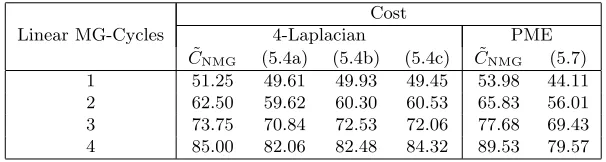
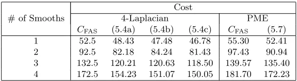
as the average time to perform one thousand residual calculations (note that the choice of coefficientα(x) has no effect on the running time). The grid for which the results are presented is a regular 512×512 triangular grid. The work unit for the 4-Laplacian was found to be 0.075s, and for the PME 0.079s, on this grid. These values were used in equations (3.19) and (3.18) to calculate the approximate execution time (denoted ˜CNMGfor Newton-MG andCFASfor FAS
multigrid).
Linear MG-Cycles
Cost
4-Laplacian PME
˜
CNMG (5.4a) (5.4b) (5.4c) C˜NMG (5.7)
[image:19.612.154.457.358.439.2]1 51.25 49.61 49.93 49.45 53.98 44.11 2 62.50 59.62 60.30 60.53 65.83 56.01 3 73.75 70.84 72.53 72.06 77.68 69.43 4 85.00 82.06 82.48 84.32 89.53 79.57
Table 1: Predicted and actual running times (s) for the execution of 100 Newton iterations with varying numbers of linear V-cycles applied to the model problems from section 5
# of Smooths
Cost
4-Laplacian PME
[image:20.612.160.451.73.153.2]CFAS (5.4a) (5.4b) (5.4c) CFAS (5.7) 1 52.5 48.43 47.48 46.78 55.30 52.41 2 92.5 82.18 84.24 81.43 97.43 90.94 3 132.5 120.21 120.63 118.50 139.57 135.40 4 172.5 154.23 151.07 150.05 181.70 172.23
Table 2:Predicted and actual running times (s) for the execution of 100 FAS V-cycles with varying numbers of smooths applied to the model problems from section 5
The results in table 2 show that the theoretical bound is not as accurate for the FAS iteration for the 4-Laplacian as it is for Newton-MG, but the estimate is better for the PME. The estimates for the 4-Laplacian are pessimistic because the cost of calculating the Jacobian diagonals is less than double the cost of calculating the residual for the 4-Laplacian, whereas it is much closer to double for the PME.
In the calculation of the linearisation we note that we perform more calcu-lations per element in Newton-MG than in FAS and so reuse calculated values more often. Therefore there is a greater opportunity for computational savings naturally available for inexact Newton iterations which is not the case for FAS. The theoretical bound is therefore likely to be approximated more sharply in the case of FAS the more complicated an operator becomes. This highlights that the Newton-MG is likely to become faster (per iteration) compared to FAS for more complex nonlinear operators.
In section 3 the prediction was made that the ratio between the per V-cycle execution time for FAS compared to Newton-MG, when performing three linear V-cycles per Newton iteration and three pre- and post-smoothing steps per FAS V-cycle, would be approximately 5.4. LetCNMG(4L) (CNMG(PME)) represent the actual cost for the 4-Laplacian problem (5.4a) (PME) per linear V-cycle using three linear iterations per Newton step, andCFAS(4L)(CFAS(PME)) the actual cost for the 4-Laplacian problem (5.4a) (PME) using three pre- and post-smoothing iterations in the FAS iteration. Then
CFAS(4L)
CNMG(4L) ≈5.09 and
CFAS(PME)
CNMG(PME) ≈5.85.
The running times of a single iteration of each of the algorithms does not tell us about the convergence behaviour of the algorithms. In the next subsections we present results for the FAS and Newton-MG iterations that demonstrate the stability and efficiency of the algorithms.
6.2. 4-Laplacian
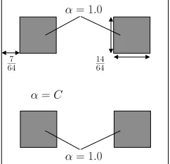
We consider the solution of the 4-Laplacian problems (5.4a), (5.4b) and (5.4c) on the domain Ω≡(0,1)2. The coefficient function α is piecewise
con-stant, and the distribution of the coefficient on the domain is shown in figure 1. The right-hand side is chosen such that the exact solution isu∗
whenα(x)≡1.0. The results in this section are presented where the initial ap-proximationu(0)= 0.7u∗
. A note is made at the end what effect using a nested iteration (cf. [12, 48]) to obtain an initial approximation on the finest grid has on the convergence of the two methods. The coarsest uniform grid on which the discontinuities in the coefficient function are fully captured (i.e. all discontinu-ities coincide with element edges) is a 64×64 grid. In the bulk of the domain the functionα takes some constant valueC, and in the shaded regions we fix
α= 1.0. From the theory in [44] we know that convergence of a linear multigrid iteration will not be independent of the size of the jump in the coefficient when a localquasi-monotonicityproperty [44] fails to hold on coarse grid levels. In the example given this occurs for the case whereC <1. In the case whereC > 1 the convergence of a linear multigrid iteration will be independent of the jumps in the coefficient. We should therefore find that convergence of the Newton-MG iteration deteriorates for decreasingC <1, and may find that the convergence is independent of the size of the jumps in the coefficient for the case C > 1. There exists no theory to suggest how FAS should perform.
α=C
14 64 7
64
α= 1.0
[image:21.612.245.366.280.397.2]α= 1.0
Figure 1: Sample distribution ofαon the domain Ω≡(0,1)2
Figures 2a and 2b show the number of V-cycles required to reduce the initial residual in the approximation by a factor of 10−7. Absence of any point from
the graphs indicates non-convergence. In figure 2a convergence is not obtained for problems (5.4a) and (5.4c) for values ofC <10−2. As predicted by the linear
theory the Newton-MG algorithm breaks down for decreasingC <1. For values ofC >1 we find that the convergence of the nonlinear iteration is independent of the size of the jump in the coefficient. We see similar behaviour for the FAS multigrid algorithm, except that the algorithm is significantly less stable for small values of C. For larger values of C the number of V-cycles required for convergence is comparable in the two cases.
A representative set of running times on different grids for problem (5.4b), using the distribution of αgiven in figure 1 with C = 105, is shown in figure
10−4 10−2 100 102 104 106 10 15 20 25 30 35 40 C Linear V−Cycles Newton−MG (5.4a) (5.4b) (5.4c)
(a) Number of linear V-cycles for conver-gence of 4-Laplacian type problems with
αas in figure 1
10−4 10−2 100 102 104 106 10 15 20 25 30 35 40 FAS C FAS V−Cycles (5.4a) (5.4b) (5.4c)
(b) Number of FAS V-cycles for conver-gence of 4-Laplacian type problems with
[image:22.612.141.468.74.265.2]αas in figure 1
Figure 2: Convergence of Newton-MG and FAS multigrid cycles for 4-Laplacian type problems on a 512×512 grid
FAS. In practice we find that (due to the fact that the implementation requires time to set up various approximations; (de-)allocate memory; perform I/O; and other operations) the actual speed up for the Newton-MG iteration is 3.12. For problems in which more Newton / FAS iterations need to be performed we find that the execution time of the nonlinear iterations will begin to dominate the overall running time and we will see a move towards the predicted improvement in running times.
10−1 100 101 102 103 Grid Size Time (s)
642 1282 2562 5122 10242 20482 Newton−MG FAS Slope 1
(a) Running time of 4-Laplacian for Newton-MG and FAS multigrid for the caseC= 105
in figure 1
10−1 100 101 102 103 104 Grid Size Time (s)
322 642 1282 2562 5122 10242
Newton−MG Newton−GMRES FAS Slope 1
(b) Execution time for FAS and Newton-MG for the PME with time-step ∆t=h
for grid spacingh
Figure 3: Comparison of execution times for model problems
[image:22.612.138.465.376.548.2]convergence behaviour of the FAS multigrid iteration seems to be very similar to that of the Newton-MG iteration in the case of using pointwise (non)linear smoothers.
We make a note on how the two methods are applied in a nested iteration (cf. [12, 48]), as this is often useful in practice to obtain an initial approxi-mation on a fine grid. In the nested iteration, approxiapproxi-mations are interpolated from coarse grids to finer grids, where a number of iterations of some iterative solution method are performed on each grid in order to obtain a ‘good’ initial approximation to the solution on the next finest grid. It is well known that in practice the convergence of a Newton iteration may not be monotonic, unless an approximation is in a ball of guaranteed convergence. On the other hand the authors have not observed a situation in which the FAS iteration does not converge monotonically (assuming it converges). FAS can be used effectively within a nested iteration, with often only a single FAS iteration required to give a ‘good’ approximation on the next finest grid. However, it may be the case that several Newton iterations are required to obtain the same reduction in the residual gained by the first FAS iteration. Hence the relative cost of perform-ing a nested iteration with the FAS algorithm may be less than performperform-ing a nested iteration with Newton’s method. However, it is still expected that the running time of a Newton iteration is superior to an FAS iteration if a nested approximation is used.
The problem of finding a ‘good’ initial approximation may be of some concern for the case of an elliptic type problem, such as the p-Laplacian, but is not important in the time dependent setting, where a good initial approximation may be gained using information from the solution at the previous time-step. Results are presented in the next section demonstrating the superiority of a Newton-MG iteration over the FAS iteration for a time dependent problem. 6.3. Porous Medium Equation (PME)
In this section we present results for Newton-MG, FAS and a Newton method where the linear system is approximated by a multigrid preconditioned GMRES iteration (Newton-GMRES) applied to the PME for the case where the solution is a self-similar solution of Barenblatt [3]
u(x, t) = 1
µ2 "
max
(
1−
µ r
r0µ ¶2
,0
)#m1
,
r=
q x2
1+x22, µ= µ
t t0
¶2(1+1m)
, t0= r02m
4(1 +m),
(6.1)
settingm = 2. We solve this on the domain Ω≡(−1,1)2, and impose
it is shown that, for a Lipschitz continuous solutionu to the porous medium equation, the convergence rate deteriorates proportional to the grid spacing. To prevent the error in the time derivative from dominating the time step should be taken proportional to the grid spacing, and hence the nonlinear multigrid methods remain of optimal order. We note that (6.1) is not Lipschitz continu-ous, but we still observe the same optimal behaviour (cf. table 3 and figure 3b). The restriction on the time-step also holds in the case of FAS, and the maximum allowable time-step (i.e. the largest time-step for which each nonlinear method gives a convergent iteration) for the FAS is bounded by the maximum allowable time-step for a corresponding Newton iteration. This supports the conjecture put forward in section 4.3 that convergence of the FAS iteration is dependent on the convergence of a Newton iteration.
Grid Size Backward Euler Crank-Nicolson
MG FAS GMRES MG FAS GMRES
32×32 0.255 0.101 >10 0.348 0.111 >10 64×64 0.0930 0.0389 >10 0.0828 0.0560 6.74 128×128 0.0189 0.0147 4.01 0.0215 0.0158 0.544 256×256 0.00732 0.00599 0.242 0.00968 0.00702 0.138 512×512 0.00340 0.00282 0.0353 0.00452 0.00311 0.0423 1024×1024 0.00140 0.00120 0.0114 0.00193 0.00134 0.0145 2048×2048 0.000669 0.000627 0.00417 0.000924 0.000702 0.00568
Table 3: Maximum allowable time-step (s) for FAS and inexact Newton iterations for the PME with exact solution given by (6.1) withr0= 0.3
Results are also presented for a multigrid preconditioned Newton-GMRES iteration. The preconditioner is a single V-cycle applied to the symmetric part of the Jacobian. From table 3 we see that the GMRES iteration gives a more stable algorithm. From figure 3b we see that there is very little extra cost in performing the GMRES iteration for a large increase in the stability of the method. The results for the multigrid-preconditioned GMRES iteration are included to demonstrate that it is relatively simple to increase the stability of an inexact Newton method by utilising a more suitable linear inner iteration. This flexibility is not present for the FAS multigrid. Even changing the smoother from the pointwise Jacobi to a pointwise Gauss-Seidel gives a large increase in the execution time of the algorithm.
In order to model materials with different diffusivities on the domain we may introduce a piecewise constant coefficient function, similar to that used in the 4-Laplacian (cf. (5.4a)). The problem to solve is then given by
ut=∇ ·(αum∇u).
term dominates. The distribution of the coefficientαon the domain again has the same effect as described for the 4-Laplacian (results not shown), and as predicted in [44].
The execution time of the algorithms is optimal with regard to the grid spacing (cf. figure 3b) with the execution time of the Newton-MG being quicker than that of the FAS iteration. On a 512×512 grid and 1024×1024 grid the execution time for the Newton-MG iteration has stabilised to be a little more than twice as fast as the FAS iteration.
7. Conclusions
The results presented here suggest that a Newton-MG method should be preferred over an FAS iteration for reasons of:
i Efficiency: The Newton-MG iteration may be much more efficient than an FAS iteration. In particular the theory in section 3 shows that as a nonlin-ear operator becomes more complicated, the cheaper the Newton iteration becomes with respect to a work unit Wl on a grid Ωl. This does not hold
true for the FAS iteration. We also observe a faster execution time for Newton-MG in practice.
ii Stability: The stability of the Newton method appears slightly better than that of an FAS iteration and numerical experiment supports a conjecture made in section 4 that the convergence of an FAS iteration requires the convergence of a Newton iteration.
iii Flexibility: There is far greater flexibility to choose components in the al-gorithm for an inexact Newton method. In particular, FAS is a solver for elliptic and parabolic problems. On the other hand Newton’s method may be used in conjunction with a suitable linear iteration that is preconditioned by multigrid. This may increase robustness and can provide a basis for solving a wider range of PDEs.
In any multigrid algorithm the operator that is most important for conver-gence of the algorithm is the smoothing operator. Changing the smoother in the linear case does not require frequent updates of the linear operator or residual, and hence one incurs less heavy cost penalties when choosing more sophisticated smoothers. In the nonlinear setting, even choosing a nonlin-ear pointwise Gauss-Seidel iteration as a smoother requires a considerable amount of work to update the nonlinear residual after each pointwise up-date. Hence, for the FAS, a faster execution time, relative to a work unit, is observed for simple problems in which a pointwise Jacobi smoother is appropriate.
theory can be used to infer how a Newton-MG iteration will perform for a nonlinear problem. Sophisticated algorithms may be developed by tak-ing advantage of the knowledge of these two methods individually, such as the truncated non-smooth Newton multigrid [20]. In addition, there are no spectral variants of the FAS such as algebraic multigrid (cf. [48]), and no methods such as monotone and truncated multigrid methods [30, 31] which can be used to take advantage of certain properties of the underlying operator, or to overcome difficulties presented by the underlying operator. There are some situations, however, in which the FAS iteration may be of more use than a Newton iteration. The memory requirements are less for the FAS iteration than for a Newton iteration, as the (large) sparse Jacobian matrices do not need to be stored in memory [33, 34, 47]. In situations in which memory requirements are an issue Jacobian-free Newton-Krylov (JFNK) methods [29] provide a less memory-intensive way of implementing an approx-imate Newton-Krylov method. Implementations include multigrid precondi-tioned GMRES variants, e.g. [19, 39]. However, JFNK methods do not remove the need to store at least a preconditioning matrix (if preconditioning is to be performed). For very large problem sizes it could be the case that there is not enough memory available to perform an approximate Newton iteration, but there is for an FAS iteration. In this situation an FAS iteration would be preferred.
The conclusions drawn here have been shown to hold in the case of simple systems of equations (cf. [33–35]), but should hold for more complex systems of equations as well. The estimates for the relative execution times can be used for adaptively refined grids and hierarchies in which the grids are non-overlapping, so long as the number of points on each grid is estimated accurately enough.
This paper gives a framework for assessing the performance of nonlinear multigrid methods in the case of a scalar nonlinear equation implemented se-quentially. It would be interesting to observe in more detail how the algorithms perform in the case of systems of equations and implementations in parallel, which can be the basis for future investigations.
8. Acknowledgements
We would like to thank Robert Scheichl and Eike M¨uller for valuable discus-sions, in particular regarding the theory of multigrid methods. The first author acknowledges the EPSRC for their financial support.
[1] M. Baines, M. Hubbard, P. Jimack, A. Jones, Scale-invariant moving fi-nite elements for nonlinear partial differential equations in two dimensions, Applied Numerical Mathematics 56 (2006) 230–252.
[3] G. Barenblatt, Scaling, self-similarity, and intermediate asymptotics: di-mensional analysis and intermediate asymptotics, volume 14 of Cambridge Texts in Applied Mathematics, Cambridge University Press, 1996.
[4] P. Bastian, O. Ippisch, F. Rezanezhad, H. Vogel, K. Roth, Numerical simu-lation and experimental studies of unsaturated water flow in heterogeneous systems, in: W. J¨ager, R. Rannacher, J. Warnatz (Eds.), Reactive Flows, Diffusion and Transport, Springer Berlin / Heidelberg, 2005.
[5] D. Braess, Finite Elements: Theory, fast solvers, and applications in solid mechanics, second ed., Cambridge University Press, 2001.
[6] J. Bramble, D. Kwak, J. Pasciak, Uniform convergence of multigrid V-cycle iterations for indefinite and nonsymmetric problems, SIAM Journal of Numerical Analysis 31 (1994) 1746–1763.
[7] J. Bramble, J. Pasciak, J. Wang, J. Xu, Convergence estimates for multigrid algorithms without regularity assumptions, Mathematics of Computation 57 (1991) 23–45.
[8] J. Bramble, J. Pasciak, J. Wang, J. Xu, Convergence estimates for product iterative methods with applications to domain decomposition, Mathematics of Computation 57 (1991) 1–21.
[9] A. Brandt, Multilevel adaptive solutions to boundary value problems, Mathematics of Computation 31 (1977) 333–390.
[10] A. Brandt, Rigorous local mode analysis of multigrid, in: Preliminary Proc. 4th Copper Mountain Conf. on Multigrid Methods, Copper Mountain, Col-orado.
[11] S. Brenner, L. Scott, The Mathematical Theory of Finite Element Methods, number 15 in Texts in Applied Mathematics, 3rd ed., Springer, 2008. [12] W. Briggs, V. Henson, S. McCormick, A Multigrid Tutorial, 2nd ed.,
Soci-ety for Industrial and Applied Mathematics, 2000.
[13] J. Brown, B. Smith, A. Ahmadia, Achieving textbook multigrid efficiency for hydrostatic ice sheet flow, SIAM Journal on Scientific Computing 35 (2013) B359–B375.
[14] P. Deuflhard, Newton Methods for Nonlinear Problems: Affine Invariance and Adaptive Algorithms, number 35 in Springer Series in Computational Mathematics, Springer Berlin / Heidelberg, 2004.
[16] M. Donatelli, M. Semplice, S. Serra-Capizzano, Analysis of multigrid pre-conditioning for implicit PDE solvers for degenerate parabolic equations, SIAM Journal on Matrix Analysis and Applications 32 (2011) 1125–1148. [17] M. Donatelli, M. Semplice, S. Serra-Capizzano, AMG preconditioning for
nonlinear degenerate parabolic equations on nonuniform grids with applica-tion to monument degradaapplica-tion, Applied Numerical Mathematics 68 (2013) 1–18.
[18] P. Gaskell, P. Jimack, M. Sellier, H. Thompson, Efficient and accurate time-adaptive multigrid simulation of droplet spreading, International Journal for Numerical Methods in Fluids 45 (2004) 1161–1186.
[19] L. Ge, F. Sotiropoulos, A numerical method for solving the 3D unsteady incompressible navier-stokes equations in curvilinear domains with complex immersed boundaries, Journal of Computational Physics 225 (2007) 1782– 1809.
[20] C. Gr¨aser, R. Kornhuber, Multigrid methods for obstacle problems, Journal of Computational Mathematics 27 (2009) 1–44.
[21] J. Green, P. Jimack, A. Mullis, J. Rosam, An adaptive, multilevel scheme for the implicit solution of three-dimensional phase-field equations, Numer-ical Methods for Partial Differential Equations 27 (2011) 106–120.
[22] W. Hackbusch, Multi-Grid Methods and Applications, volume 4 ofSpringer Series in Computational Mathematics, Springer-Verlag, 1985.
[23] W. Hackbusch, Comparison of different multi-grid variants for nonlinear equations, Zeitschrift f¨ur Angewandte Mathematik und Mechanic 72 (1992) 148–151.
[24] W. Hackbusch, A. Reusken, On global multigrid convergence for nonlinear problems, in: W. Hackbusch (Ed.), Robust Multi-Grid Methods, Notes on Numerical Fluid Dynamics, Vieweg, Braunschweig, 1988, pp. 105–113. [25] W. Hackbusch, A. Reusken, Analysis of a damped nonlinear multilevel
method, Numerische Mathematik 55 (1989) 225–246.
[26] V. Henson, Multigrid methods for nonlinear problems: An overview, in: Proceedings of the Society of Photo-Optical Instrumentation Engineers (SPIE), pp. 36–48.
[27] G. Jouvet, C. Gr¨aser, An adaptive Newton multigrid method for a model of marine ice sheets, Journal of Computational Physics 252 (2013) 419–437. [28] T. Kim, J. Pasciak, P. Vassilevski, Mesh-independent convergence of the
[29] D. Knoll, D. Keyes, Jacobian-free Newton-Krylov methods: a survey of approaches and applications, Journal of Computational Physics 193 (2004) 357–397.
[30] R. Kornhuber, Monotone multigrid methods for elliptic variational inequal-ities I, Numerische Mathematik 96 (1994) 167–184.
[31] R. Kornhuber, Monotone multigrid methods for elliptic variational inequal-ities II, Numerische Mathematik 72 (1996) 481–499.
[32] S. MacLachlan, C. Oosterlee, Local Fourier analysis for multigrid with over-lapping smoothers applied to systems of PDEs, Numerical Linear Algebra with Applications 18 (2011) 751–774.
[33] D. Mavriplis, Multigrid approaches to non-linear diffusion problems on un-structured meshes, Numerical Linear Algebra with Applications 8 (2001) 499–512.
[34] D. Mavriplis, An assessment of linear versus non-linear multigrid methods for unstructured mesh solvers, Journal of Computational Physics 175 (2002) 302–325.
[35] J. Molenaar, Multigrid Methods for Fully Implicit Oil Reservoir Simulation, Technical Report, TWI, Delft University of Technology, 1995.
[36] J. Murray, Mathematical Biology: An Introduction, 3rd ed., Springer, 2002. [37] A. Napov, Y. Notay, Smoothing factor, order of prolongation and actual
multigrid convergence, Numerische Mathematik 118 (2011) 457–483. [38] J. Ortega, W. Rheinboldt, Iterative Solution of Nonlinear Equations in
Several Variables, Computer Science and Applied Mathematics, Academic Press, 1970.
[39] H. Park, D. Knoll, R. Rauenzahn, C. Newman, J. Densmore, A. Wollaber, An efficient and time accurate, moment-based scale-bridging algorithm for thermal radiative transfer problems, SIAM Journal on Scientific Computing 35 (2013) S18–S41.
[40] A. Reusken, Convergence of the multigrid full approximation scheme for a class of elliptic mildly nonlinear boundary value problems, Numerische Mathematik 52 (1988) 251–277.
[41] A. Reusken, Convergence of the multilevel full approximation scheme in-cluding the V-cycle, Numerische Mathematik 53 (1988) 663–686.
[43] Y. Saad, Iterative Methods for Sparse Linear Systems, 2nd ed., Society for Industrial and Applied Mathematics, 2003.
[44] R. Scheichl, P. Vassilevski, L. Zikatanov, Multilevel methods for elliptic problems with highly varying coefficients on non-aligned coarse grids, SIAM Journal on Numerical Analysis 50 (2012) 1675–1694.
[45] M. Semplice, Preconditioned implicit solvers for nonlinear PDEs in monu-ment conservation, SIAM Journal on Scientific Computing 32 (2010) 3071– 3091.
[46] V. Shaidurov, Multigrid Methods for Finite Elements, 2nd ed., Kluwer Academic Publishers, 1995.
[47] L. Stals, Comparison of non-linear solvers for the solution of radiation transport equations, Electronic Transactions on Numerical Analysis 15 (2003) 78–93.
[48] U. Trottenberg, C. Oosterlee, A. Sch¨uller, Multigrid, Academic Press, 2001. [49] E. Vecharynski, A. Knyazev, Absolute value preconditioning for symmetric indefinite linear systems, SIAM Journal on Scientific Computing 35 (2013) A696–A718.
[50] R. Wienands, W. Joppich, Practical Fourier Analysis for Multigrid Meth-ods, Chapman and Hall/CRC, 2005.
[51] D. Xie, New nonlinear multigrid analysis, in: Seventh Copper Mountain Conference on Multigrid Methods, pp. 793–808.