Adaptation in the forest deer mouse:
evolution, genetics, and development
The Harvard community has made this
article openly available.
Please share
how
this access benefits you. Your story matters
Citation Kingsley, Evan Prentice. 2015. Adaptation in the forest deer mouse: evolution, genetics, and development. Doctoral dissertation, Harvard University, Graduate School of Arts & Sciences.
Citable link http://nrs.harvard.edu/urn-3:HUL.InstRepos:17467192
Terms of Use This article was downloaded from Harvard University’s DASH repository, and is made available under the terms and conditions applicable to Other Posted Material, as set forth at http://
© Evan Prentice Kingsley
Dissertation Advisor: Hopi Hoekstra Evan Prentice Kingsley
Adaptation in the forest deer mouse: evolution, genetics, and development
Abstract
Variation in the shape, size, and number of segments along the vertebral column underlies a
vast amount of vertebrate diversity. Although the molecular pathways controlling vertebrate
segmentation during normal development are well understood, the genetic and developmental
underpinnings responsible for the tremendous variation in size and number of vertebrae are
relatively unexplored. The main goal of this dissertation is to explore the genetic and developmental
mechanisms influencing naturally occurring variation in the vertebral column. To this end, I focus
on intraspecific skeletal variation, with an emphasis on tail length, in the deer mouse, Peromyscus
maniculatus. In Chapter 1, I employ a phylogeographic framework to show that longer tails have
evolved independently in different populations of forest-dwelling mice. Closer investigation of the
underlying morphology shows that long-tailed mice have both (1) a greater number of tail vertebrae
and (2) individually longer vertebrae, compared to ancestral short-tailed mice. Chapter 2 explores the
genetic basis of tail length variation. I use quantitative trait locus mapping to uncover six loci that
influence differences in total tail length (3 associated with vertebral length and 3 with vertebrae
number). Finally, in Chapter 3 I combine comparative data from quantitative measurements of tissue
dynamics during somitogenesis in fixed embryos and ex vivo explant culture to show that embryos of
forest mice make more segments because they produce more presomitic mesoderm, and not because
of any significant difference in the timing of somitogenesis. Together, this work integrates
phylogeographic, genetic, and developmental studies to pinpoint the ways that natural selection
modifies development to produce the repeated evolution of an evolutionarily important trait, and
Introduction
If we want to understand why two branches of life look or behave differently—essentially,
why organisms are the way they are—we must uncover the paths those organisms took to become
what they are. But these paths have multiple scales. At the evolutionary level, the direction of
evolutionary change depends entirely on what already exists: evolution is a historically contingent
process that is constrained by the past. On another level, evolution has, through selective and
neutral processes, shaped patterns of genetic change through time. And on yet another scale, these
genetic changes, as molded by evolution, remodel the body of multicellular organisms by modifying
the process of development. In the spirit of the integrative nature of evolutionary change, in this
dissertation I explore evolutionary, genetic, and developmental aspects of adaptive skeletal variation
in the deer mouse, Peromyscus maniculatus.
Because all evolutionary variation begins as intraspecific variation, understanding the genetic
underpinnings of local adaptation is especially relevant to the study of adaptive traits. There are two
main advantages to exploring evolutionarily important traits within a species. The first is conceptual:
all evolutionarily important differences among species originated as intraspecific variation, which is a
compelling argument for the importance of understanding the origin and fate of polymorphic
variation within species. The second is practical: a variety of approaches to uncover the loci
underlying phenotypic differences—QTL mapping, for example—can only be applied to differences
between interfertile organisms, i.e. those of the same, or very closely related, species. On the other
hand, the obvious downside to studying intraspecific variation is that there is not often that much of
it. Necessarily, the vast majority of evolutionary change is not present within a species but has
accumulated between species. By exploring the genetic and developmental mechanisms underlying
variation that has evolved over small time scales, i.e., within a species, we may gain insight into
Intraspecific variation in P. maniculatus is a rewarding source for studies of adaptation. Deer
mice have been studied for over one hundred years in a natural historical context (e.g. Dice 1941;
Blair 1950) and the abundant adaptive phenotypic variation present across the continent-wide range
of this species has, in the last ten years, led to a number of fruitful investigations into the genetic
basis of adaptive traits, including cryptic pigmentation (Linnen et al. 2009, 2013) and high-altitude
adaptation (Storz et al. 2007, 2009; Cheviron et al. 2012)
This dissertation fits into a set of classic natural history observations about two ecotypes
within deer mice: the forest and prairie forms. As early as Osgood’s (1909) revision of the genus,
researchers have classified this species into forest forms and prairie forms: the former having longer
tails and larger hind feet (Dice 1940; Blair 1950), which Horner (1954) showed, through an extensive
set of observational and manipulative experiments, to be correlated with climbing ability. Though
some work has suggested that the forms may be partially reproductively isolated in some locations
(Dice 1931; Hooper 1942) and mice from some forest populations show strong habitat preference
(Harris 1952; Wecker 1963), more recent work has shown substantial gene flow at microsatellite loci
across habitat interfaces (Yang & Kenagy 2011). The fact that differences in foot and tail length
persist in the face of strong gene flow suggests that natural selection acts strongly to maintain
variation in these traits.
The genetic architecture of adaptive traits is of special interest to evolutionary biologists.
Here, I investigate the numbers and effects of loci underlying differences in skeletal morphology,
with a special interest in the vertebral column of the tail, with the goal of understanding how
underlying genetic architecture and genetic correlations can influence the evolution of complex traits
(Klingenberg 2008; Flint & Mackay 2009; Armbruster 2014). The genetic architecture of skeletal
variation has been extensively studied in the laboratory mouse (e.g. Cheverud et al 2001;
body size, but the genetic architecture of traits may be different in natural and artificial selection
regimes (Mackay 2001; Hansen 2006). The genetics of naturally selected skeletal variation has been
studied extensively in sticklebacks (e.g. Shapiro et al. 2009; Miller et al. 2014), but few studies have
examined the genetic architecture of adaptive skeletal variation in mammals.
Variation in the vertebral column underlies an enormous amount of vertebrate diversity and,
though much attention has been paid to how the identities of vertebrae shift through changes in
development (e.g. Burke et al. 1995), less is known about the developmental and evolutionary
changes that can generate differences in segment number. Gomez et al. (2008) recently showed that
differences in the timing of the segmentation clock correlate with the massive disparity in segment
number between snakes and mice, and Kimura et al. (2012) suggest that differences in somite size
may influence vertebral number differences in medaka, but evidence regarding the developmental
basis of vertebral number evolution is scant. Thus, the adaptive difference in caudal vertebrae
number between forest and prairie deer mice examined in this dissertation is a unique opportunity to
study the evolutionary, genetic, and developmental bases of differences in vertebral number in a
mammal.
Outline of the dissertation
Chapter 1 explores intraspecific convergent evolution of the forest deer mouse in
geographically distant populations. I show that long-tailed forest mice are evolving independently in
eastern and western regions of the species range, and that, when accounting for non-independence
of populations within a species, mice in forests do indeed have longer tails than prairie mice. I go on
to investigate the skeletal nature of forest-prairie tail length differences and find that both eastern
and western forest populations have longer vertebrae and a greater number of vertebrae in their tails
natural populations, I show that number and length are not genetically correlated: a population of
recombinant individuals from a forest-prairie intercross shows no correlation of vertebral counts
with vertebral length. Together, these results show that independently evolving populations of forest
mice have converged on the long-tail phenotype by similar morphological mechanisms—increasing
number and length of skeletal elements—despite these mechanisms being genetically unconnected.
In Chapter 2, I investigate the genetic basis of this skeletal variation. Using an F2
forest-prairie intercross population, I explore structures of genetic correlations among bone traits and
uncover morphological modules that are genetically coupled. I then employ a quantitative trait locus
(QTL) mapping approach to map loci influencing tail length trait variation. Six major-effect loci
control tail length variation in this cross. These loci coincide with loci underlying the tail’s
constituent traits: three of the six overlap vertebral count loci and the other three coincide with loci
affecting vertebral length. Additionally, at all six tail-length loci the forest allele has a positive effect
on tail length, further supporting the idea that natural selection maintains tail length variation in deer
mice. Finally, I identify candidate genes from QTL intervals and discuss the implications of
polygenic architecture on tail length evolution.
Chapter 3 examines the developmental mechanisms underlying variation in vertebral number
in deer mice. Variation in the number of somites, the earliest developmental precursor to vertebrae,
could be due to differences in timing of somitogenesis, differences in rates of posterior growth in
the embryo, or both. By observing segmentation in ex vivo tail explant cultures, I show that there is
no difference in the timing of somite formation in forest and prairie embryos. I present evidence
that the segment number difference between forest and prairie deer mice is due to a difference in the
rate of posterior outgrowth, specifically in the rate of presomitic mesoderm shortening, and that the
evidence, I discuss future directions for developmental investigations of segment number variation
Chapter 1
Convergent evolution of long-tailed forest deer mice
Evan P. Kingsley1, Krzysztof Kozak2, and Hopi E. Hoekstra1
1Department of Organismic and Evolutionary Biology, Museum of Comparative Zoology, Howard Hughes Medical Institute
Harvard University, 26 Oxford Street, Cambridge, Massachusetts 02138, USA and Department of Molecular and Cellular Biology
Harvard University, 16 Divinity Avenue, Cambridge, Massachusetts 02138, USA
INTRODUCTION
Convergent evolution occurs when similar phenotypes evolve in different lineages.
Convergence has been defined at both ends levels of biological organization: at the smallest, most
specific scale, the same phenotypes can be produced by the exact same mutations occurring in
different lineages, thereby producing identical genetic and morphological outcomes; i.e. true
parallelism. But at a larger scale, convergence is also defined simply as natural selection favoring
similar phenotypes in different lineages, with nothing implied about the underlying biological
mechanisms. The level at which convergent evolution occurs—whether two lineages fix the same
adaptive mutation, different mutations at the same gene, different genes in the same biochemical
pathway, or by totally different genetic mechanisms—informs us about the ways that selection and
constraint influence evolutionary outcomes (Arendt & Reznick 2008; Manceau et al. 2010; Elmer &
Meyer 2011).
Variation among populations of the deer mouse, Peromyscus maniculatus, provides a system for
understanding the organismal basis of convergent evolution by local adaptation. This species has the
widest range of North American mammals (Hall 1981) and populations are adapted to their local
environments in many parts of the range. This variation has served for the basis of several studies of
the genetics of adaptive traits (e.g. Snyder 1981 and Storz et al. 2007, Dice 1941 and Linnen et al.
2009), and the repetition of similar selective pressures in geographically distant parts of its range
suggest the possibility of repeated convergent adaptations. Previous authors have placed deer mouse
populations into two roughly-defined categories: forest-dwelling and prairie-dwelling (Osgood 1909,
Blair 1950). Mice in these categories are differentiated behaviorally and morphologically: mice found
in forests tend to have smaller home ranges (Howard 1949, Blair 1942), bigger ears, longer hind feet,
northerly and southerly parts of the species range, respectively (Fig. 1); it is thought that P.
maniculatus populations expanded northward into forests following the Pleistocene glaciation (King
1968; Hall 1981) and thus that the deer mouseancestor was a prairie form.
It is not known whether the widespread forest populations reflect a single origin of the
forest morphology that has spread across the continent, or if the forest phenotype has evolved by
convergent evolution, i.e., selection acting independently in different populations to produce local
adaptation. Previous work on the phylogenetic relationships among deer mouse subspecies has
suggested convergence—allozyme (Avise et al. 1979) and mitochondrial studies (Lansman et al.
1983; Dragoo et al. 2006) have shown there to be a split between eastern and western populations—
but no studies or which we are aware have explicitly considered morphological and ecological
context in a continent-wide sampling. Additionally, mitochondrial-nuclear discordance is common in
this species (e.g., Taylor & Hoffman 2012), which complicates the interpretation of mitochondrial
studies when traits of evolutionary interest, in this case skeletal variation, are likely controlled by loci
in the nuclear genome. Furthermore, though previous work has compared the morphology of forest
and prairie mice from different populations, these studies have not accounted for the fact that
populations do not represent statistically independent sources of data due to shared evolutionary
history and gene flow between those populations (reviewed by Stone et al. 2011).
Previous work has shown that deer mice use their tails extensively while climbing. Horner
(1954) carried out a survey of climbing behavior in Peromyscus, and found not only a correlation
between tail length and climbing ability, but also provided experimental evidence that within P.
maniculatus, forest mice are more reliant on their tails for their climbing proficiency than their
short-tailed counterparts. Smartt and Lemen (1980) showed that, within populations of two other
Peromyscus species, tail length correlates with degree of arboreality, and climbing ability was shown to
Here, we investigate the evolution of the deer mouse tail in two complementary ways. First,
we reconstruct phylogeographic relationships among populations of P. maniculatus to test hypotheses
about the convergent evolution of tail length. We show that forest-dwelling deer mice do not belong
to a single phyletic group or genetic cluster and thus that forest forms are convergent. We also show
that longer tails are correlated with forest habitation, even when taking account of shared history
and gene flow among populations. Then we investigate the morphological basis of tail length
differences in two geographically distant convergent populations, implicating similar but
quantitatively different mechanisms for the generation of these differences. Finally, we show that,
despite correlation in the wild, differences in the constituent traits of tail length between forest and
prairie mice can be genetically separated in the lab. Together, these results strongly suggest that
natural selection maintains multiple locally adapted forest populations, and sets a stage for further
investigations of the genetic and developmental bases of an adaptive skeletal trait.
METHODS
Morphometric measurements from museum specimens
Records of P. maniculatus were downloaded from the Mammal Network Information System
(MaNIS; www.manisnet.org) and the Arctos database (www.arctos.database.museum/home.cfm).
We inspected all specimens available at Harvard's Museum of Comparative Zoology. As nearly all
specimens were present in the collection as stretched skins, we considered the original collector’s
data to be the most reliable source of measurements. Juvenile specimens were excluded based on the
characteristic grey pelage.
We excluded all specimens labeled as “juvenile”, “subadult” or “young adult” or having any
tail abnormalities or injuries. We also deleted any individuals with total length below 106 mm or tail
Figure 1. Deer mouse geography and tail length variation. A. Map of North America showing the roughly defined range of P. maniculatus. Forest and prairie range limits were obtained from Osgood (1909) and Hall (1981). Dots show locations from which we have samples and the style of the dots show 1) the GIS land cover-defined habitat of the sites and 2) which analyses they were used in. The dashed outline for “x-ray samples” indicates that we used samples from those locations for our comparison of vertebral number and length (see Figure 4). The red circle indicates that the population was used in the intraspecific contrasts analysis for FST estimates (see Figure 3). B. Box-and-whisker plot of tail:body length ratio variation among deer mice subspecies in museum collections. Box color indicates habitat, as described for each subspecies by Hall 1981; tan = prairie, grey = intermediate, green = forest. Note that these do not always match the land cover-defined habitat designations.
luteus bairdii blandus rufinus nebrascensis fulvus borealis gambelii sonoriensis rubidus gracilis abietorum nubiterrae 0.6 0.8 1.0 1.2
ratio of tail length to body length
−120 −110 −100 −90 −80 −70
20
30
40
50
abietorum
gambeliigambeliigambelii gambelii nubiterrae sonoriensissonoriensis nebrascensis gambelii gambelii rubidus borealis gracilis blandus borealis borealis borealis bairdii bairdii nebrascensis fulvusfulvus nubiterrae sonoriensis sonoriensis rufinus blandus rubidus gambelii gracilis luteus bairdii luteus A B forest range prairie range
land cover forest land cover prairie
Peromyscus maniculatus has highly stable subspecies ranges and subspecific identity can be
determined reliably based on appearance and location (Gunn & Greenbaum 1986; Hall 1981; King
1968). We scanned the original distribution maps from Hall (1981) and georeferenced them in
ArcGIS v. 9.2 (ESRI 2007). Subspecies were then assigned based on original identification where
available and on mapping the coordinates digitally. Subspecies with fewer than three specimens
available were excluded.
Morphometric statistics from museum specimens
We calculated two types of dependent variables. Ratios of tail length to body length were
used as a simple representation of the relation between the two measurements. We also applied a
linear transformation of the data to address potential non-linear scaling of the two lengths (Fox &
Weisberg, 2011). We fitted a linear model of tail length vs. body length. 30 individuals were randomly
selected from each subspecies with over 30 records available in order to reduce bias resulting from
large number of records for some common subspecies. We fitted log, square and Box-Cox
transformations of the response variable and included quadratic and cubic terms for the predictor.
All possible models were compared using ANOVA and the adjusted R2 values. Due to very low fit
of the best model (R2 = 0.11) we decided that simple ratios are an appropriate test statistic. The
normality of the ratio distribution was rejected with p < 0.001 using the Kolmogorov-Smirnoff test.
We therefore used the non-parametric Mann-Whitney U Test to compare the ratios between
arboreal and non-arboreal mice. We used the car package (Fox & Weisberg 2011) in R (R
Development Core Team 2005) for all computation.
We extracted DNA (Qiagen DNeasy kit) from of 25-50 mg of liver from 78 individuals that
comprise samples from our lab collections, loans from other researchers, and from museum tissue
loans (see Appendix for details) and combined this with data from another ongoing study in the
Hoekstra Lab for a total of 104 samples. The sampling encompassed the range of P. maniculatus and
included 33 locations. We assigned animals to habitat types based on their sampling locations: we
used ArcGIS (ESRI) to extract land cover, i.e., habitat type, information from the North American
Land Change Monitoring System 2010 Land Cover Database (NALCMS, 2010) with a 1 km-radius
buffer around each sampling location. We split land cover categories into forest and
non-forest/prairie designations for all analyses: we called classes 1-6 and 14 forest (Temperate or
sub-polar needleleaf forest, Sub-sub-polar taiga needleleaf forest, Tropical or sub-tropical broadleaf
evergreen forest, Tropical or sub-tropical broadleaf deciduous forest, Temperate or sub-polar
broadleaf deciduous forest, Mixed Forest, Wetland) and others non-forest/prairie (Tropical or
sub-tropical shrubland, Temperate or sub-polar shrubland, Tropical or sub-sub-tropical grassland, Temperate
or sub-polar grassland, Cropland, Urban and Built-up).
Array-based capture and sequencing of short-read libraries
To assess genome-wide population structure, we used an array-based capture library and
sequenced region-enriched genomic libraries using the Illumina platform (Gnirke et al. 2009). Our
MYbaits (MYcroarray; Ann Arbor, MI) capture library sequences have 5114 randomly chosen
regions of the Peromyscus maniculatus genome averaging 1.5kb in length (5.2Mb of unique,
non-repetitive sequence) and are identical to the regions used in Domingues et al. (2012) and Linnen et
al. (2013). We extracted genomic DNA using DNeasy kits (Qiagen; Germantown, MD) or the
Autogenprep 965 (Autogen; Holliston, MA) and quantified using Quant-it (Life Technologies).
and Illumina sequencing libraries were prepared and enriched following Domingues et al. (2012) and
Linnen et al. (2013). Briefly, we prepared multiplexed sequencing libraries in five pools of 16
individuals each using a “with-bead” protocol (Fisher et al. 2011) and enriched the libraries
following the MYbaits protocol. We pulled down enrichment targets with magnetic beads
(Dynabeads, Life Technologies), PCR amplified with universal primers (Gnirke et al. 2009), and
generated 150bp paired end reads on a HiSeq2000 (Illumina Inc.; San Diego, CA).
Short-read sequence analysis
To process the capture-enriched sequence data, we used custom Python software available at
github.com/brantp/. In brief, this software uses Stampy to map merged paired-end reads to the P.
maniculatus genome scaffolds (Baylor 2012 version) and then combines reads, by individual, into
BAM files with Picard (broadinstitute.github.io/picard/). We then used GATK (McKenna et al.
2010; DePristo et al. 2011) to call variants with UnifiedGenotyper in a larger sample of maniculatus
individuals. We filtered these variants for those present in more than 75% in our 106 individuals and
with GQ>20. This filtering produced 12721 variants.
Genetic principal components analysis (PCA)
To assess population structure across the range of P. maniculatus, we used SMARTPCA and
TWSTATS (Patterson et al. 2008) with the genome-wide SNP data from the enriched short-read
libraries described above. We condensed the significant principal components (eigenvectors) by
multidimensional scaling in the Python module scikit-learn (Pedregosa et al. 2011) into two
dimensions for Figure 3A. To visualize genetic relationships inferred by the PCA, we generated a
significant eigenvectors of the SMARTPCA output. The Python code to produce bootstrapped trees
can be found at github.com/kingsleyevan/phylo_epk.
Within-species comparative analysis
Samples from different populations within a species are non-independent because of shared
ancestry and gene flow (Stone et al. 2011), so we must consider these factors when analyzing
phenotypes across populations. We used two measures of genetic similarity to control for this
non-independence. First, we pared our data down to populations from which we had three or more
individuals and estimated global mean and weighted FST between populations using the method of
Weir and Cockerham (1984) as implemented in VCFtools (Danecek et al. 2011) (see “in population
contrasts” in Appendix). Second, we used a measure of genetic similarity (“--relatedness2” in
VCFtools: the kinship coefficient of Manichaikul et al. 2010) between all individuals in the dataset
for which we have tail and body measurements (“in individual contrasts” in Appendix). For both the
population- and individual-level analyses, we used a general linear mixed model approach, as
implemented in the R package MCMCglmm (Hadfield 2010), to test for an effect of habitat
(forest/prairie) on population average tail:body ratio or individual tail:body ratio when including FST
or kinship coefficient as a random effect.
Vertebral morphometrics of wild-caught specimens
We x-ray imaged the skeletons of wild-caught mice from four populations (see Appendix for
specimen details) with a Varian x-ray source and digital imaging panel in the Museum of
Comparative Zoology Digital Imaging Facility. Then we used ImageJ’s segmented line tool to
measure the lengths of each individual vertebra, starting from the first vertebra and proceeding
vertebral column is not always clear, so for consistency’s sake we call the first six vertebrae (starting
with the first sacral-attached) the sacral vertebrae; the caudal vertebrae are all the vertebrae posterior
to the sixth sacral vertebra.
Because tail length scales with body size in our sample, we fitted a linear model with the lm
function in R (R Development Core Team 2005) to adjust all vertebral length measurements for
body size. We regressed total tail length (R2 = 0.62) and the lengths of individual vertebrae (R2 =
0.14–0.59) on the sum length of the six sacral vertebrae, and used the residuals from the linear fit for
all subsequent analyses. We obtain similar results when we regress length measurements on femur
length instead of sacral vertebral length (results not shown).
F2 intercross trait correlation analysis
All mice bred in this cross were in the Hoekstra lab colony at Harvard University. We
obtained prairie deer mice, P. m. bairdii, from the Peromyscus Genetic Stock Center (University of
South Carolina), which we crossed with forest deer mice, P. m. nubiterrae, from Westmoreland
County, Pennsylvania. We mated one male and one female of each subspecies—two mating pairs,
one in each direction—and used their offspring to establish 10 F1 sibling mating pairs. We x-ray
imaged 96 F2 offspring from these F1 pairs and measured them as described in the “Vertebral
morphometrics. . .” section above and we used the lm function in R to assess correlations in the
resulting measurements. All animals were between 80 and 100 days old when measured.
RESULTS
Non-monophyly of forest forms
We used an array-based capture approach to resequence and call SNPS in >5000 genomic
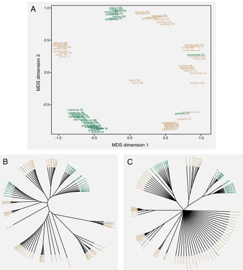
Figure 2. Genetic principal components analysis shows that forest forms are not a single genetic group.A. Multi-dimensional scaling (MDS) of genetic PCA into two dimensions. B. Neighbor-joining tree based on Euclidian distances in PCA-space allows visualization of genetic clustering. C. Same as B, but with clades collapsed that are not present in >50% of 1000 bootstrap replicates. Note that forest forms from the east and west do not cluster. Color indicates GIS land cover-defined habitat (tan = prairie, green = forest).
rubidus OR rubidus OR rubidus OR rubidus OR
rubidus ORrubidus OR rubidus OR rubidus OR rubidus CA
gambelii OR gambelii OR
gambelii ORgambelii ORgambelii OR
gambelii OR gambelii OR nebrascensis WY nebrascensis UT rufinus NM rufinus NM sonoriensis AZ sonoriensis AZ sonoriensis AZ sonoriensis CA blandus NM blandus NM blandus NM blandus NM
blandus CHborealis AB
fulvus VE fulvus TL
blandus NMblandus NM
bairdii NE bairdii NE
nubiterrae PA
abietorum ME nubiterrae PAnubiterrae PA
nubiterrae PA nubiterrae PA nubiterrae PA gracilis ON gracilis ON gracilis MI gracilis MIgracilis MI gracilis MI gracilis MIgracilis MIgracilis MI gracilis ON nubiterrae PA nubiterrae VA sonoriensis CA gambelii CA gambelii CA gambelii CA
gambelii CAgambelii CA
gambelii CA gambelii CA gambelii CA
gambelii CA borealis AB
borealis ABborealis AB
blandus CH gambelii OR gambelii OR 1.0 0.5 0.0 -0.5
-1.0 -0.5 0.0 0.5 1.0
luteus NE gambelii CA sonoriensis AZ rubidus OR blandus NM nebrascensis UT rubidus CA blandus NM bairdii SD bairdii SD nubiterrae PA rubidus OR sonoriensis CA luteus NE gambelii OR gracilis MI bairdii SD rubidus OR bairdii SD fulvus VE rufinus NM luteus NE luteus NE bairdii NE nubiterrae PA nebrascensis UT rubidus OR bairdii SD gambelii CA gracilis ON bairdii SD luteus NE luteus NE luteus NE bairdii SD gracilis MI gambelii OR sonoriensis AZ luteus NE gracilis MI luteus NE luteus NE rubidus OR nebrascensis WY blandus NM gambelii CA abietorum ME lueus NE fulvus TL bairdii SD gracilis ON nubiterrae PA blandus NM gambelii CA borealis AB gambelii CA gambelii OR gambelii OR
rubidus OR nubiterrae PA
gambelii OR blandus CH luteus NE luteus NE gambelii CA gambelii OR luteus NE gracilis ON gambelii CA gambelii OR gambelii OR gambelii OR rubidus OR nubiterrae PA bairdii SD gracilis MI nubiterrae PA blandus NM luteus NE borealis AB rubidus OR luteus NE blandus NM bairdii SD gracilis MI
luteus NE luteus NE
nubiterrae VA nubiterrae PA gracilis MI gracilis MI luteus NE gambelii CA rubidus OR luteus NE sonoriensis CA gambelii CA borealis AB sonoriensis AZ blandus NM rubidus OR sonoriensis CA bairdii SD nebrascensis UT bairdii SD gambelii OR luteus NE luteus NE bairdii SD gambelii OR luteus NE luteus NE blandus CH sonoriensis AZ rufinus NM nubiterrae PA blandus CH nubiterrae PA gambelii OR luteus NE borealis AB nebrascensis WY gracilis ON luteus NE gambelii OR gambelii OR gambelii CA gambelii CA abietorum ME bairdii NE rubidus CA blandus NM gambelii OR nubiterrae PA gambelii OR rubidus OR gambelii CA bairdii SD rubidus OR bairdii SD sonoriensis CA fulvus TL nubiterrae PA gracilis MI gracilis MI borealis AB rubidus CA sonoriensis AZ gracilis ON bairdii SD gambelii CA rufinus NM rubidus OR bairdii SD rubidus OR luteus NE bairdii SD bairdii SD borealis AB fulvusVE blandus NM luteus NE nubiterrae PA luteus NE luteus NE rubidus OR nubiterrae PA blandus NM bairdii SD rubidus OR gracilis MI gracilis MI gracilis MI luteus NE bairdii NE luteus NE gambelii CA luteus NE gambelii OR luteus NE blandus NM gambelii CA luteus NE luteus NE gracilis MI rubidus OR blandus NM nubiterrae PA nubiterrae VA borealis AB gambelii CA gracilis ON luteus NE sonoriensis AZ gracilis MI luteus NE gambelii CA luteus NE rubidus OR gambelii CA luteus NE gambelii OR nebrascensis UT
A
B
C
MDS dimension 2
resequenced regions, we explored genetic similarity among the sampled individuals by genetic
principal components analysis (PCA) (Patterson et al. 2008).
Genetic PCA methods show that individuals from forests (we determined habitat, forest vs.
non-forest, using GIS land cover data, as described in Methods, above) do not compose a single,
monophyletic group. Instead, we see the mice of the putatively derived forest forms clustering with
nearby non-forest forms. To visualize the distances among individuals in the genetic PCA, we
generated a neighbor-joining tree from MDS-scaled distances (Fig. 2B). In 1000 bootstrap replicates
of this tree (a 50% majority rule tree is shown in Fig. 2C), none produced a tree in which forest mice
formed a single group. These results show that forest forms are evolving independently in eastern
and western parts of the species range.
Variation in tail length correlates with habitat
To assess whether differences in the length of the tail are significant even when accounting
for non-independence of populations created by gene flow and shared ancestry, we included
measures of genetic similarity among populations and individuals in a set of generalized linear mixed
models. In these models, we ask whether animals in different habitats have significantly different
tail:body ratios when including measures of genetic similarity as random effects.
First, we considered whether forest and prairie populations of differ in their mean tail
lengths. When taking pairwise FST (Fig. 3) between populations (Appendix) into account, we find
that habitat has a significant effect in our mixed model (p = 0.002 for weighted mean FST, p < 0.001
for global mean FST; fit by Markov Chain Monte Carlo [Hadfield 2010]). Next, we assessed whether
individuals from forest and prairie habitats differ in tail length when accounting for genetic
similarity. We find a significant effect of habitat on tail:body ratio in our mixed model with kinship
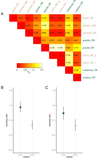
model-Figure 3. Tail length differs between habitats even when accounting for genetic non-independence. A. Matrix of genome-wide mean FST between populations used in the within-species comparative analysis (see Appendix for
samples used). Larger values indicate more allele-frequency difference between two populations; smaller values indicate more similarity. B. Tail:body length ratios for each population predicted by a generalized linear mixed model taking genetic differentiation (FST) between populations into account. C. Tail:body length ratios for prairie and forest
individuals predicted by a similar model as in B, but with pairwise genetic relatedness (kinship coefficient [Manichaikul et al. 2010]) between individuals taken into account. Error bars in B and C represent 95% confidence intervals.
bairdii_SD blandus_NM gambelii_ORgracilis_ON gracilis_MIluteus_NE_g luteus_NE_inubiter rae_ PA rubidus_OR rubidus_OR nubiterrae_PA luteus_NE_i luteus_NE_g gracilis_MI gracilis_ON gambelii_OR blandus_NM bairdii_SD 0 0 0.103
0 0.140 0.039
0 0 0.140 0.039
0 0.150 0.150 0.086 0.112
0 0.071 0.076 0.076 0.057 0.061
0 0.040 0.098 0.018 0.018 0.092 0.015
0 0.033 0.075 0.136 0.042 0.042 0.126 0.051
0 0.035 0.012 0.042 0.103 0.013 0.013 0.096 0.030
0 0.05 0.1 0.15
[image:22.612.149.465.82.594.2]predicted population means in Figure 3B and the predicted individual means by habitat in Figure 3C.
Together, these results robustly show that, even when taking non-independence of populations into
account, deer mice from forested habitats do indeed have longer tails than those from prairie
habitats.
Convergence in skeletal morphology
We x-rayed specimens from two pairs of geographically distant forest-prairie populations
(see Figure 1 and Appendix) and measured their vertebrae. These four populations were chosen
because individuals from the two forest populations (West forest [rubidus] and East forest [nubiterrae])
are each more closely related to a nearby non-forest population than they are to each other (Figure
2), thereby representing independently evolving forest populations. We measured the total tail
length, the lengths of the longest caudal vertebra and the number of caudal vertebrae and found
that, in both comparisons, forest mice had 1) significantly longer tails (Wilcoxon test, East: W = 49,
p < 0.001; West: W = 49, p < 0.001) significantly longer vertebrae (Wilcoxon test, East: W = 49, p
< 0.001; West: W = 49, p < 0.001) significantly more vertebrae (Wilcoxon test, East: W = 49, p <
0.002; West: W = 49, p-value < 0.003) than their nearby prairie form (Fig. 4). Importantly, forest
forms 1) do not have different numbers of trunk vertebrae (all samples had 18 or 19), and 2) we
performed all these tests on body-size-corrected data, which means that these forest-prairie
differences are specific to the tail. Additionally, when we compared the lengths of the individual
caudal vertebrae along the tail we found that not all caudal vertebrae are longer in the forest than in
prairie mice. In the eastern population pair, caudal vertebrae 4 through 15 had median lengths in the
forest mice than the longest caudal vertebra in prairie mice. The corresponding segment in the
Figure 4. Convergent tail vertebral morphology in eastern and western forest-prairie population pairs. A. Forest mice have more caudal vertebrae than prairie mice in the east and west. Horizontal red lines represent medians. B.
Forest mice have longer vertebrae than prairie mice in the east and west. Dashed line represents the median length of the longest prairie vertebra; the segment of the forest tail with longer vertebrae is 4–16 and 4–15 for western and eastern populations, respectively. C. Summary of tail vertebral differences between forest and prairie mice. Lines represent mean cumulative tail lengths. Dashed line is the cumulative length of the mean prairie tail with three extra vertebrae added, which represents an estimate of the maximum contribution of difference in number of vertebrae to the difference in
0 5 10 15 20 25
0 20 40 60 80 100
0 5 10 15 20 25
1 5 10 15 20 25
1 5 10 15 20 25
0 20 40 60 80 100
cumulative tail length (mm)
0 2 4 6 ve rteb
ra length (mm)
0 2 4 6 subspecies subspecies
vertebra number vertebra number
West East 21 22 23 24 25 26 27 bairdii nubiterrae 21 22 23 24 25 26 27 gambelii rubidus n
umber of caudal
ve
rteb
We also estimated the relative contributions of differences in vertebral length and vertebral
number to the overall difference in tail length. To do this, we simulated the forest and prairie mice
having an equal number of vertebrae by inserting three long vertebrae into the center of the prairie
tails. These simulated “prairie+3” tails compensated for 42% and 53% of the average difference in
overall tail length between the eastern and western forms, respectively (Fig. 4C). These figures
represent an upper bound of the contribution of the difference in vertebral number relative to
vertebral length in these populations. Finally, a linear model of the form total length ~ longest vertebra
length + number of caudal vertebrae has an R2 = 0.98, suggesting that differences in length of vertebrae
and number of vertebrae are the main factors contributing to differences in total tail length.
Vertebrae length and vertebrae number are genetically separable
In the four populations examined above, both forest populations have both 1) longer caudal
vertebrae and 2) more caudal vertebrae. Could these differences be correlated in natural populations
because they are under the control of the same genetic loci? To test this hypothesis, we generated 96
F2 recombinant individuals from an intercross between P. m. nubiterrae and P. m. bairdii and generated
x-ray images from each individual. Using these images, we measured the correlation between the
length of the longest caudal vertebra and the number of caudal vertebrae. We detect no significant
correlation (Fig. 5; t = 0.87, df = 94, p = 0.39) between vertebral length and vertebral number in the
tails of our F2 animals (96 individuals allows an 80% probability of detecting a correlation of r >
0.25 at p < 0.05).
DISCUSSION
The “convergence” in an episode of convergent evolution can occur on many different
Figure 5. No significant correlation between number and length of caudal vertebrae in a laboratory F2
intercross. Each point is represents the length of the longest caudal vertebra and the number of caudal
vertebrae measured from a radiograph of an F2 nubiterrae x bairdii individual. 96 individuals allows 80% power to detect a correlation of r > 0.25.
20 21 22 23 24 25
3.5 4.0 4.5 5.0
length of longest vertebra
n
umber of
ve
rteb
phenotype’s repeated evolution allows us to make inferences not only about the selective conditions
under which the phenotype evolves but also about the constraints that limit the production of
variation in that phenotype. Repeated evolution of a phenotype usually implies two
non-mutually-exclusive explanations: 1) there are intrinsic limits to the phenotypic variation that can be produced,
to the extent that similar phenotypes are a frequent outcome of neutral evolution, or 2) similar
selection pressures favor similar phenotypic adaptations. In both the neutral and selected cases, the
repeated evolution of the phenotype can be due to similar or identical evolution at any level: the
same gross phenotypic change could be produced in different evolutionary lineages by identical
genetic mutations, similar changes in tissue morphogenesis, similar environmental changes that
induce convergent phenotypic change, or anything in between. Only for the case in which selection
plays a role, however, are similar phenotypic changes induced by the enhanced survival and/or
reproduction of individuals with those phenotypes. It is this case in which we are most interested—
understanding the organismal response to repeated bouts of selection allows insight into the process
of adaptation that studying a single instance does not.
In his 1950 survey of adaptive variation in Peromyscus, W. Frank Blair wrote that the forest
form of P. maniculatus “ranges through the Appalachians from northern Georgia northward and
extends on northward to Labrador.” He discussed the two main forms—one grassland and one
forest—as two separate groups when he continued: “It ranges across the continent in the Canadian
forests…and extends south through the Rocky Mountains and the mountains of the Pacific coast….
The grassland form occupies the grasslands of the interior of the continent and is surrounded on
three sides by the long-tailed forest type.” Other authors have also described the two forms of P.
maniculatus as single, separate entities (Osgood 1909) and the work of Dice (1931) and Hooper
(1942) suggested that the two forms failed to interbreed, suggesting that forest deer mice might
Since those studies, several investigations have inferred the relationships among populations
of P. maniculatus using molecular data. Avise et al. (1979) surveyed biochemical variation in 21
allozymes and showed that there is a broad similarity in allele frequencies in populations spanning
most of the range of P. maniculatus. They report that “gene flow among widely separated populations
of P. maniculatus cannot account for the similarity of their allelic contents. Either the populations of
P. maniculatus have not been separated long enough for greater differentiation to have occurred by
chance, and/or some form of natural selection is acting to help maintain similarity in electromorph
configuration.”
These conclusions are broadly consistent with subsequent studies that used restriction sites
in mitochondrial DNA (Lansman et al. 1983) and mitochondrial DNA sequences (Dragoo et al.
2006) to show, though these reports did not explicitly explore forest-prairie dynamics, that
well-supported phylogenetic clades are reconstructed that contain forest and prairie subspecies,
sometimes with identical mitochondrial haplotypes. Though consistent in the sense that they do not
recover monophyletic forest or prairie clades, the mtDNA studies conflict with the allozyme study
in two ways: first, the specific topologies of the trees/networks are different, but second, and more
importantly, Avise et al. report populations with some of the highest allozyme heterozygosities that
had been reported at that time, while Lansman et al. recovered monomorphic mtDNA clades from
those same populations.
This cytonuclear discordance was explicitly studied in deer mice populations on the west
coast of the United States by Yang and Kenagy (2009) and in the Upper Peninsula of Michigan by
Taylor and Hoffman (2012). Both studies found significant disagreement between patterns of
genetic differentiation as determined at nuclear microsatellite loci versus mitochondrial sequence,
Lansman et al. 1983; Dragoo et al. 2006), suggest that relationships based on mtDNA sequence may
not be as relevant as patterns of nuclear genomic differentiation for studies of ecological adaptation.
In the present study, we examine the phylogeography of P. maniculatus in the context of
intraspecific ecological adaptation, and specifically in the framework of the classic forest-prairie
dichotomy that has been recognized in this species for over one hundred years. Previous
phylogeographic studies that have considered samples from across the range of P. maniculatus have
only tangentially discussed adaptation, but we explore the phylogeography of the species using >
12000 genome-wide markers and examine correlation between habitat and morphology, making the
current study the first to explicitly study the adaptation to forest habitats in P. maniculatus in a
continent-wide sample. We chose to use a non-tree-based method, genetic principal components
analysis (PCA), given the difficulty of constructing bifurcating phylogenetic relationships among
intraspecific samples from populations experiencing gene flow.
The results of our genetic PCA are concordant with those of previous studies that found
that forest mice are not a single monophyletic group. The pattern of genomic differentiation we see
in our PCA data is roughly similar to that recovered by Avise et al. (1979), with a group of
populations from eastern North America that are clearly separated from populations in the western
half of the continent. But we also see some less expected patterns. Individuals from forest
populations of the east, subspecies nubiterrae and gracilis, have the greatest affinity to the blandus
populations from New Mexico and Mexico (Fig. 2B-C).
When we assigned habitat values to those populations using GIS land cover data, we found
that populations captured in forest habitats have longer tails than those in non-forest habitats, when
taking gene flow among populations into account. Thus, we support the interpretation of this
pattern made by Lansman et al. (1983): “It is thus very probable that the currently recognized
more likely that environmental selection pressures have led to the independent evolutionary
appearance of these two morphs in different maniculatus lineages.” Our data support at least two,
one eastern and one western, independently evolving groups of forest P. maniculatus—western North
American populations are less differentiated from each other than they are from those in the east,
making it difficult to confirm more than a single group of forest mice in the west.
We show that the eastern and western forest forms are convergently evolving at the
population level. By this, we mean that similar environments—forests—appear to favor similar
phenotypes—long tails—in two phylogenetic groups that are not closely related to each other (in
terms of population differentiation within this species). Furthermore, in two forest-prairie
population pairs, one eastern and one western, we find that both pairs differ in the two components
of the caudal skeleton that could vary to produce differences in tail length, namely the number of tail
vertebrae and the length of those vertebrae. This coupling of vertebral length and vertebral number
could be explained in two ways: 1) number and length of vertebrae are controlled by identical, or
linked, regions of the genome, or 2) multiple genetic variants controlling number and length of
vertebrae have independently fixed in eastern and western populations.
To distinguish between these hypotheses, we examined 96 F2 individuals from a laboratory
intercross between a forest form, P. m. nubiterrae, and a prairie form, P. m. bairdii. If differences in the
length and number of vertebrae are controlled by variants in the same region(s) of the genome, we
expect them to be correlated in the F2 individuals. On the other hand, if the two traits are under
control of variants in different genomic regions, recombination during the production of gametes in
the F1 parents should decouple these traits in the F2 generation, and we should detect no
correlation between these traits. We find the latter: we detect no significant correlation between
number and length of vertebrae in the F2 (Fig. 5). This result implies that forest environments have
populations. It may be advantageous, biomechanically, to have more and longer caudal vertebrae
when climbing, or it may be simply that longer tails are favored, and alleles affecting length and
number were present in the source population from which the forest mice evolved, and thus alleles
affecting both traits increased in frequency from standing genetic variation in these populations.
There is some precedent to variation in number and length of vertebrae being produced by
separate genetic mechanisms. Rutledge et al. (1974) performed a selection study in which they
applied selection on body length and tail length in replicate mouse strains. The authors found that,
in two replicate lines selected for increased tail length, one line had evolved a greater number of
vertebrae and the other evolved longer vertebrae. That the number and lengths of vertebrae can be
genetically uncoupled may not be surprising, given the timing of processes in development that
affect these traits. The process of somitogenesis, which creates segments in the embryo that presage
the formation of vertebrae, is completed in the Mus embryo by 13.5 days of development (Tam
1981), while the formation of long bones does not begin until much later in embryogenesis and
skeletal growth continues well into the early life of the animal. Chapters 2 and 3 of this dissertation
investigate the genetic and developmental bases of these morphological differences.
In this study, we aimed to explore the possible convergent evolution of an adaptive
phenotype within a species. We confirmed that long-tailed forest-dwelling deer mice are evolving
independently in eastern and western parts of its range, and that tail length does indeed differ in
forest versus prairie habitats. Furthermore, we showed that longer tails, in both eastern and western
forest mice, are due to convergent differences in the number of caudal vertebrae and the lengths of
those vertebrae. Finally, we show that, despite the observation that caudal vertebrae number and
length evolve in tandem in our natural population samples, the genetic mechanisms producing those
differences can be decoupled in a lab intercross. Together, these results put over one hundred years
phylogeographic footing, along with establishing a framework for studying the genetic basis of local
Chapter 2
QTL mapping of skeletal traits in Peromyscus maniculatus reveals the genetic basis of arboreal adaptation
Evan P. Kingsley1, Lorena Benitez2, and Hopi E. Hoekstra1
1Department of Organismic and Evolutionary Biology, Museum of Comparative Zoology, Howard Hughes Medical Institute
Harvard University, 26 Oxford Street, Cambridge, Massachusetts 02138, USA and Department of Molecular and Cellular Biology
Harvard University, 16 Divinity Avenue, Cambridge, Massachusetts 02138, USA
INTRODUCTION
Understanding the genetic architecture of complex traits is a key goal of evolutionary
biology. The number, effect size, dominance, and pleiotropy of loci underlying complex adaptive
traits can all significantly influence the process of evolution, and, furthermore, the architecture itself
can evolve (Hansen 2006; Rajon & Plotkin 2013). Recent studies have leveraged powerful
approaches like quantitative trait locus mapping and genome-wide association studies to gain insight
into the evolution of a variety of complex traits in a variety of organisms from social organization of
ants (Purcell et al. 2014) to diet in sticklebacks (Arnegard et al. 2014), to burrow construction in
oldfield mice (Weber et al. 2013).
Examining genetic correlations among traits can inform our understanding of how
adaptation proceeds in natural populations (Klingenberg 2008; Armbruster et al. 2014).
Measurements of two traits that share the same underlying genetic or developmental mechanisms
will covary. This morphological integration among traits can constrain evolution: a particular value
of one trait may be favored by natural selection, but if its value covaries with that of another trait,
then its selective advantage is tied to—and perhaps constrained by—selection on the other trait
(Lande 1979, 1980). On the other hand, if the selective advantage of two covarying traits is in the
same direction as the covariance, the integration between them can promote, and even accelerate,
morphological evolution. This integration reflects a shared genetic basis for variation—pleiotropy—
and/or a shared developmental mechanism. With greater integration may come greater constraint: a
cost of complexity (Schluter 1996; Orr 2000; but see Wagner et al. 2008). In sum, the covariance
structure among traits is a key determinant of evolutionary outcomes.
Variation in the number and size of skeletal elements underlies much of mammalian
diversity (Pilbeam 2004; Asher et al. 2011). Previous studies seeking to understand the genetic basis
strains (Morris et al. 1999; Cheverud et al. 2001; Wada et al. 2000), but the patterns of pleiotropy for
alleles fixed by natural selection may be different from those fixed by the strong artificial selection in
the laboratory (Otto 2004). Crucially, an allele’s likelihood of fixation by natural selection may
depend on the particular pattern of pleiotropy for that allele (Orr 2000; Welch & Waxman 2003;
Otto 2004). It is unclear whether we should expect patterns of trait correlation and pleiotropy to be
similar between even closely related taxa. Perhaps they should be similar: much of mammalian
development comprises similar mechanisms tweaked by evolution to produce different forms. On
the other hand, patterns of pleiotropy are known to be allele-specific. Indeed, mutations in different
parts of the same gene—cis-regulatory versus protein-coding regions, for example—are expected to
have different pleiotropic effects (Stern 2000; Stern and Orgogozo 2008).
In this chapter, we investigate the genetics of adaptive skeletal differences between
populations of the deer mouse, Peromyscus maniculatus. There exists extensive intraspecific variation in
this species, and much of it is proposed to be the result of local adaptation (see Chapter 1). This
implies that natural selection has favored different alleles that are now at high frequency in different
populations, despite the homogenizing effect of gene flow among populations experiencing
divergent selective regimes. Deer mice in forests have longer tails than their prairie counterparts and
these differences reliably exist across environmental gradients from forest to prairie (Chapter 1; Blair
1950; Yang & Kenagy 2011) and the longer tail of the forest deer mouse is used extensively when
climbing (Horner 1954).
The longer tails of forest deer mice have more vertebrae and longer vertebrae than those of
prairie deer mice. Importantly, these differences are specific to the tail: the number and lengths of
trunk vertebrae are not significantly different between forms (Chapter 1). Though these traits are
correlated in natural populations, we have shown that variation in number and length of caudal
and prairie deer mice are accompanied by differences in the size of the hind foot (Blair 1950; Horner
1954), also thought to be an important factor in arboreal locomotion. Here, we explore variation in
limb and tail traits, examine how traits covary in an experimental cross, and map loci underlying
variation in those traits, all in the context of evolutionary adaptation of complex traits.
METHODS
F2 intercross
To establish our genetic mapping population, we established crosses between prairie (P. m.
bairdii) and forest (P. m. nubiterrae) deer mice. The bairdii mice were descendants of mice obtained
from the Peromyscus Genetic Stock Center (University of South Carolina), originally from prairie
habitat in Washtenaw County, Michigan. The nubiterrae were descendants of 18 wild-caught mice that
we captured from maple-birch forest in Westmoreland County, Pennsylvania, in 2010. The mapping
cross consisted of two families: one cross in each direction (family “0”: female bairdii x male
nubiterrae; family “1”: female nubiterrae x male bairdii). Each family began with two mice, one of each
subspecies. Because the alleles for most skeletal traits act in a codominant manner in the F1
offspring (Fig. 6B-D), we used an F2 intercross design for QTL mapping (Lynch and Walsh 1998).
We established 14 F1 breeding pairs, which produced 495 F2 animals for analysis. When F2s
reached 70-120 days old, they were sacrificed, measured for gross morphology (total length, tail
length, ear length, hind foot length, and mass), and radiographed in the Museum of Comparative
Zoology Digital Imaging Facility (MCZ DIF).
Morphometric statistics
This study is concerned with the bones of the tail and limbs. We and other authors have
that two subspecies of P. maniculatus, nubiterrae and bairdii, differ in a number of skeletal traits (see
Chapter 1 of this dissertation and references therein). We measured these traits in four individuals
each of nubiterrae and bairdii, 14 F1 animals, and 495 F2 animals by measuring x-ray radiographs. We
used a digital x-ray system (Varian Medical Systems, Inc.; Palo Alto, CA) to obtain radiographs of
whole specimens mounted such that plane containing the anterio-posterior and medio-lateral axes
was orthogonal to the imaging plane. We measured all traits with Fiji/ImageJ (Schindelin et al. 2012;
Rasband 1997–2014) using an included standard to determine scale. Figure 6A describes how we
measured each trait. We performed all analyses in R (R Core Team 2008), performed principal
components analysis (PCA) using the psych (Revelle 2015) package, and used ggplot2 (Wickham 2009),
reshape2 (Wickham 2007), scales (Wickham 2014), and RColorBrewer (Neuwirth 2014) packages to
display data.
We measured the lengths of 68 bone traits (67 are bone lengths and 1 is a count, caudal
vertebra number) (Fig. 6). Most bone length traits were correlated with body size in our cross, so we
corrected for body size using linear regression on sacrum length. Sacrum length represents a
standard for body size (sacrum length vs. body mass: Pearson’s r = 0.55, 95% CI: 0.48–0.60; vs.
ruler-measured body length: r = 0.62, 95% CI: 0.56–0.67) and a section of the vertebral column that
is anterior to the caudal vertebrae and that does not significantly differ between subspecies
(Wilcoxon test, W = 38, p = 0.1). We corrected for body size by regressing raw trait measures
against the sum length of the six sacral vertebrae, then adding the residuals from that regression to
the trait mean to put the corrected measurements in the ranges of the raw measurements.
In previous work (see Chapter 1) we found that nubiterrae tails have 1) a larger number of
caudal vertebrae and 2) longer caudal vertebrae than the tails of bairdii. To summarize these
differences, we used three summary statistics to describe these differences: 1) the number of caudal
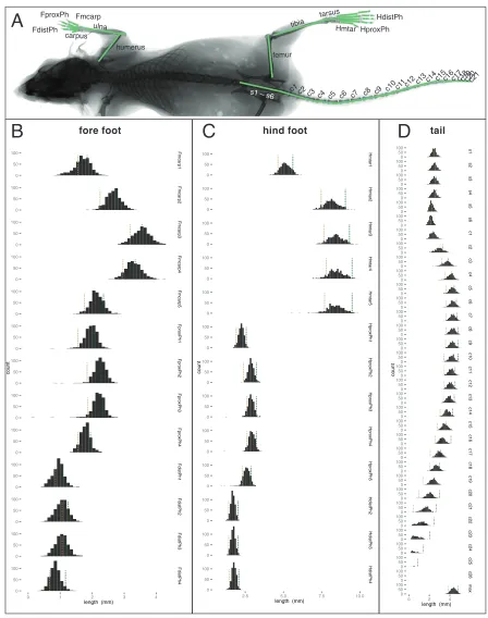
Figure 6. Trait distributions in QTL mapping cross. A. Radiograph showing traits analyzed in the F2 QTL mapping
cross. B. Histograms showing distributions of forefoot length traits in the F2. C. Hindfoot length traits in the F2. D.
Vertebral length traits in the F2; “max” is the longest vertebra in the tail. Dashed vertical lines represent parental means for each trait; green lines represent nubiterrae values and tan lines represent bairdii values.
0 50 100 0 50 100 0 50 100 0 50 100 0 50 100 0 50 100 0 50 100 0 50 100 0 50 100 0 50 100 0 50 100 0 50 100 0 50 100 Hmtar1 Hmtar2 Hmtar3 Hmtar4 Hmtar5 Hpr o xPh1 Hpr o xPh2 Hpr o xPh3 Hpr o xPh4 Hpr o xPh5 HdistPh2 HdistPh3 HdistPh4
2.5 5.0 7.5 10.0
length (mm)
count 0 50 100 0 50 100 0 50 100 0 50 100 0 50 100 0 50 100 0 50 100 0 50 100 0 50 100 0 50 100 0 50 100 0 50 100 0 50 100 Fmca rp1 Fmca rp2 Fmca rp3 Fmca rp4 Fmca rp5 Fpr o xPh1 Fpr o xPh2 Fpr o xPh3 Fpr o xPh4 FdistPh1 FdistPh2 FdistPh3 FdistPh4
0 1 2 3 4
length (mm)
count 0 50 100 0 50 100 0 50 100 0 50 100 0 50 100 0 50 100 0 50 100 0 50 100 0 50 100 0 50 100 0 50 100 0 50 100 0 50 100 0 50 100 0 50 100 0 50 100 0 50 100 0 50 100 0 50 100 0 50 100 0 50 100 0 50 100 0 50 100 0 50 100 0 50 100 0 50 100 0 50 100 0 50 100 0 50 100 0 50 100 0 50 100 0 50 100 0 50 100 s1 s2 s3 s4 s5 s6 c1 c2 c3 c4 c5 c6 c7 c8 c9 c10 c11 c12 c13 c14 c15 c16 c17 c18 c19 c20 c21 c22 c23 c24 c25 c26 max
0 2 4
length (mm)
count
A
B
fore footC
hind footD
tailFmcarp
carpus ulna
humerus
Hmtar
c1 c2 c3 c4 c5 c6 c7 c8 c9 c10c11 c12 c13 c14
c15c16c17c18c19c20c21
s1 – s6
tail, maxvert; and 3) the total length of the tail, tail_total. A model in which the former two
measurements are the explanatory variables (tail_total = vert_count + maxvert + ε) explains r2 = 0.89 of
the variance in the total length of the tail, suggesting that differences in the length and number of
vertebrae are the main constituent traits describing total tail length.
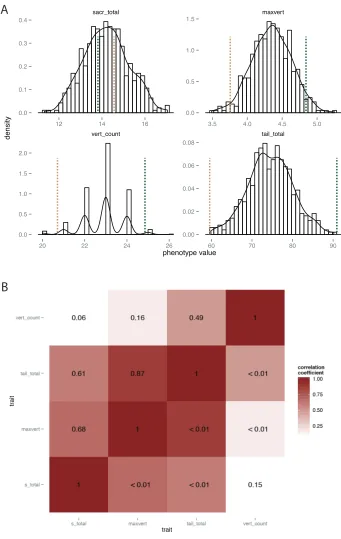
To explore which skeletal traits are influenced by the same genetic variation, we used
correlation coefficients (Pearson’s r) to explore the basic correlation structure among traits in the F2
animals. We followed that with a PCA with a varimax rotation (as implemented in the “principal”
function in the psych package in R). Before PCA, we scaled the standard deviations for each trait to 1
and centered the means of each trait to 0. Based on scree analysis, we retained the first four principal
components for F2 tail traits and F2 limb traits (see scree plots, Fig. 8B,D). The first four
components represent 82% of the variance in tail traits and 63% of the variance in limb traits.
Genotyping
We genotyped parent, F1, and F2 animals with the double digest restriction-site associated
DNA sequencing (ddRADseq) method as described in Peterson et al. (2012). Briefly, we extracted
genomic DNA from alcohol-preserved liver tissue with the AutoGenprep 965 (AutoGen; Holliston,
MA) in the Bauer Core Facility in the Harvard FAS Center for Systems Biology. We digested
genomic DNA with EcoRI and MspI (New England Biolabs; Ipswich, MA) and ligated end-specific
adapters, P1 and P2; the former includes individual barcodes, the latter is biotin labeled. Next, we
combined samples into 48-individual pools and size-selected each pool to 216-276 bp on a Pippin
Prep (Sage Science; Beverly, MA), after which we used streptavidin beads (Dynabeads M-270; Life
Technologies; Carlsbad, CA) to eliminate fragments without P2 adapters. We PCR-amplified these
pools (10 cycles) with an indexed primer. We quantified the mass of these pools using a TapeStation
5.0 nM) and combined them in equimolar ratios. We sequenced these pools in 150 bp paired-end
rapid runs on an Illumina HiSeq 2500 in the Bauer Core Facility.
To process the ddRADseq data, we used custom Python software described in Peterson et
al. (2012) and at github.com/brantp/. In brief, this software uses Stampy to map merged paired-end
reads to the P. maniculatus genome scaffolds (Baylor 2013 version) and then combines reads, by
individual, into BAM files with Picard (broadinstitute.github.io/picard/). We then used GATK
(McKenna et al. 2010; DePristo et al. 2011) to call variants with UnifiedGenotyper. From 4.3e8 raw
reads, this analysis produced 1.1e7 called variants. We hard filtered these variants for those that were
fixed in the parents of the cross, those with QD > 5, GQ > 30, and those present in more than half
the F2 individuals in our sample (using HTSeq; Anders et al. 2014). This filtering produced 4527
variants, which we used to construct the maniculatus genetic map.
Genetic map construction and quantitative trait locus (QTL) mapping
We used R/qtl to construct a linkage map for the F2 intercross between P. m. bairdii and P.
m. nubiterrae. We generated an R/qtl input file with 4527 variants using custom Python software
(github.com/brantp/rtd/vcf_to_rqtl.py) and followed the guidelines for generating linkage maps
provided by Broman and Sen (2009). We removed individuals with fewer than 1000 genotypes and
also those that were more than 90% identical. We filtered redundant markers (if a pair of markers
had identical patterns of segregation, we removed one) and removed markers that had unexpected
genotype frequencies (p < 1e-5). Using the remaining markers, we generated linkage groups using a
maximum recombination fraction of 0.35 and a minimum LOD score threshold of 10. This
produced 24 linkage groups (n of P. maniculatus is 24 [Bradshaw & George 1969]). We ordered
markers within linkage groups by permuting orders over 8-marker windows and minimizing the