Assessment of the performance of the inter-arrival time algorithm to
identify ice shattering artifacts in cloud particle probe
measurements
A. Korolev1and P. R. Field2
1Environment Canada, Toronto, Canada
2Met Office, Exeter, UK, and University of Leeds, Leeds, UK Correspondence to: A. Korolev ([email protected])
Received: 18 August 2014 – Published in Atmos. Meas. Tech. Discuss.: 8 October 2014 Revised: 22 December 2014 – Accepted: 20 January 2015 – Published: 17 February 2015
Abstract. Shattering presents a serious obstacle to current airborne in situ methods of characterizing the microphysi-cal properties of ice clouds. Small shattered fragments result from the impact of natural ice crystals with the forward parts of aircraft-mounted measurement probes. The presence of these shattered fragments may result in a significant overes-timation of the measured concentration of small ice crystals, contaminating the measurement of the ice particle size distri-bution (PSD). One method of identifying shattered particles is to use an inter-arrival time algorithm. This method is based on the assumption that shattered fragments form spatial clus-ters that have short inter-arrival times between particles, rel-ative to natural particles, when they pass through the sample volume of the probe. The inter-arrival time algorithm is a successful technique for the classification of shattering arti-facts and natural particles. This study assesses the limitations and efficiency of the inter-arrival time algorithm. The analy-sis has been performed using simultaneous measurements of two-dimensional (2-D) optical array probes with the standard and antishattering “K-tips” collected during the Airborne Ic-ing Instrumentation Experiment (AIIE). It is shown that the efficiency of the algorithm depends on ice particle size, con-centration and habit. Additional numerical simulations indi-cate that the effectiveness of the inter-arrival time algorithm to eliminate shattering artifacts can be significantly restricted in some cases. Improvements to the inter-arrival time algo-rithm are discussed. It is demonstrated that blind application of the inter-arrival time algorithm cannot filter out all shat-tered aggregates. To mitigate against the effects of shatter-ing, the inter-arrival time algorithm should be used together
with other means, such as antishattering tips and specially designed algorithms for segregation of shattered artifacts and natural particles.
1 Introduction
Ice particle size distributions (PSDs) are used in atmospheric models for computing both the radiative impact of ice clouds and the microphysical process rates that control ice cloud evolution. Therefore, an inaccurate representation of the ice PSD can have adverse impacts on the accuracy of climate and weather prediction models. Measurements of ice PSDs from aircraft-based observations form the basis of size distri-bution representations in models. Prior to entering the instru-ment sample volume, an ice particle may impact the probe’s upstream tips or inlet and shatter into many small fragments. These shattering products can then significantly contaminate measurements of airborne particle probes.
Over three decades the abundance of small ice particles measured by particle probes in the tropospheric clouds re-mained an intriguing problem. Recent studies using simulta-neous measurements of standard and modified probes (Ko-rolev et al., 2011, 2013b) have unambiguously demonstrated that in many cases measurements made with standard cloud probes are adversely affected by shattering artifacts.
shat-tered particles towards the sample volume (Korolev et al., 2013a). This method can lead to a significant reduction in the effect of shattering but is not able to completely eradicate the problem (Korolev et al., 2011, 2013b; Lawson, 2011).
The second approach is a postprocessing methodology based on the fact that shattering products are spatially clus-tered. Because of close spacing, the time difference between two successive shattered fragments passing through the sam-ple volume will be much shorter than that for naturally oc-curring particles. This time difference is usually referred to as “inter-arrival time”.
Cooper (1977) suggested that these artifacts could be fil-tered out by identifying the characteristically short inter-arrival times of particles associated with these shattering products.
Field et al. (2003) used a fast forward scattering spectrom-eter probe (FSSP) to measure particle spacing in ice clouds. The inter-arrival time distribution in ice clouds was found to have a bimodal shape with modes at 10−2and 10−4s corre-sponding to approximately 1m and 1 cm spatial separations. The particles from the long and short inter-arrival time modes corresponded to estimated concentrations of 0.1–1 cm−3and
∼100 cm−3respectively. No conclusions were drawn as to whether the latter localized clusters of high particle concen-tration were natural or artifacts. Assuming they were arti-facts, their inter-arrival time algorithm suggested average and maximum concentration overestimates of a factor of 2 and 5 respectively.
Field et al. (2006) applied an inter-arrival time algorithm (ITA) to filter out shattering artifacts, choosing a threshold inter-arrival time in the range 10−4to 10−5s, depending on the instrument and the aircraft type used for the data col-lection, to reject the short inter-arrival mode. It was found that the OAP-2DC and CIP concentrations were reduced by up to a factor of 4 when the mass-weighted mean size ex-ceeded 3 mm. The ice water content (IWC) estimate was re-duced by up to 20–30 %, most notable in cases of narrow size distributions. It was also found that the corrected PSDs could show a reduction in particle concentrations over a wide range of sizes from 200 microns for narrow distributions up to 1000 microns for the broadest distributions that are subject to the most shattering.
It should be noted that the time separation between parti-cle arrivals through the probe’s sample volume depends on true air speed. The relevant metric, which should be used to segregate shattered artifacts and natural particles is inter-particle distance along the flight direction (1x). It is ac-knowledged that the community is accustomed to referring to “inter-arrival time”1tsince this parameter is measured in the probes. In the following discussion we will be using both metrics1xand1t.
The ITA is now routinely used in two-dimensional (2-D) probe data processing to eliminate shattering artifacts (e.g., Baker et al., 2009; Lawson, 2011; Jackson et al., 2014). Moreover, it is recognized that the best practice for the
op-eration of cloud probes in the presence of ice is provided by a combination of modified tips and the application of the inter-arrival time filtering together (e.g., Korolev et al., 2011; Baumgardner et al., 2012).
While it has been demonstrated that the ITA reduces the effects of shattering, its accuracy and efficiency remains poorly quantified. For instance, can the ITA alone identify all shattering artifacts? Is the efficiency of the ITA depen-dent upon the probe specifications such as pixel resolution, response time, sample area, and inlet configuration?
Motivation for improving our understanding of the limita-tions and efficiency of the ITA is threefold. Firstly, there is a need to determine if the ITA can be used to successfully rean-alyze the historical data collected over the past thirty years. Secondly, an improved quantitative understanding of the lim-itations of the ITA will provide statements of the accuracy of the measurements of the particle number concentration, ice water content, extinction coefficient and other PSD derived parameters. Thirdly, knowledge of the efficiency of the ITA will aid in the design process of future cloud probes.
The objective of this paper is to evaluate the efficiency and limitations of ITA. A detailed description and the main as-sumptions underlying the algorithm are presented in Sect. 2. Section 3 considers general limitations of the algorithm. Analysis of the results of the OAP-2DC data processing us-ing the ITA are presented in Sect. 4. In Sect. 5 statistical sim-ulations of ice particle shattering are used to explore the lim-itations of the ITA. Finally, Sect. 6 provides a summary.
2 Description of the inter-arrival time algorithm 2.1 Basic assumptions
In the following discussion the term “shattering event” will be applied to the group of shattered fragments, that (a) formed as a result of impact of a single particle with the up-stream tips (or inlet) of a probe, and (b) at least one particle from the group of the shattered fragments was registered by the probe. It should be noted that if the particle rebounds to the sample area without shattering, it still falls in the defini-tion of the “shattering event”.
The successful application of the ITA is predicated on two basic assumptions: (1) the maximum inter-arrival time of the shattered fragments is shorter than the minimum inter-arrival time between intact particles; (2) shattered particles are al-ways passing through the sample volume as a group of no less than two particles.
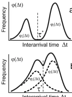
Figure 1. Conceptual diagram of the distribution of inter-arrival timesφ (1t )with well separated short and long inter-arrival time modes (a), when shattering artifacts can be segregated from the in-tact particles. When the distributions of inter-arrival time associated with intact particles φi(1t )and shattered fragmentsφs(1t )have significant overlap, then segregation of intact particles and shattered artifacts is hindered (b).
particles satisfy the condition1t < τ∗, whereas all intact par-ticles and only intact parpar-ticles are associated with 1t > τ∗
(Fig. 1a). Given this assumption it is trivial to identify the shattered artifacts and intact particles based simply on a com-parison of measured inter-arrival time1t between two suc-cessive particles and the cut-off timeτ∗.
The second assumption forms the second necessary condi-tion to identify shattered artifacts. A minimum of two closely spaced particles is necessary to allow artifacts to be identi-fied.
The conceptual diagram in Fig. 2a demonstrates these two basic assumptions about particle spacing that is required for the successful segregation of shattered artifacts and intact particles using an ITA. In reality, the challenges of image sampling and the statistical nature of particle spacings im-pose limitations on the performance of the ITA in the segre-gation of shattered artifacts and intact particles. As will be shown below, the first assumption cannot be satisfied due to statistical limitations, whereas the second condition is neces-sary but not sufficient.
2.2 Inter-arrival time algorithm
Here we describe the sequence of operations composing the basic ITA. This algorithm in its basic form will be used in the present study.
1. The inter-arrival time algorithm starts from the calcu-lations of the distribution of inter-arrival times φ (1t )
as in Fig. 1. The calculation of φ (1t ) are performed for each averaging time interval. Similar to Field et
Figure 2. Conceptual diagram of (a) idealised spatial sequence of intact particles and shattered artifacts passing through the sample volume. Case (c) when the inter-arrival time algorithm may confuse shattered artifact with intact particles, and (b, d, e, f) when intact particles may be confused with shattering artifacts.
al. (2003, 2006) the time bins inφ (1t )were logarithmi-cally spaced. The width of the time bins was optimized to trade-off accuracy of the estimation ofτ∗and the sta-tistical significance related to the number of counts in each time bin.
2. The cut-off-timeτ∗was calculated for each averaging time interval as a minimum between two maxima as-sociated with long and short time modes (Fig. 1). In cases when only one mode was present,τ∗was forced to be equal to the minimum inter-arrival time found in this averaging interval. It should be noted that the func-tionφ (1t )is a non-normalized distribution of counts in each time bin. Normalization using the bin width leads to a disappearance of the minimum between the short and long time modes inφ (1t ), which hinders calcula-tion ofτ∗.
3. Pairs of particles that satisfied the condition 1t < τ∗
were identified and marked as artifacts. It is important to note that the ITA cannot identify a single-particle shat-tered artifact (singleton) and that the minimum number of particles identified as artifacts is two.
The value ofτ∗ should be calculated for each averaging time interval. As will be shown below,τ∗has a wide dynamic range and it depends on many microphysical, environmental and instrumental parameters (Sect. 4.3). The assumption, that
τ∗remains constant, may result in large errors in identifying shattering artifacts.
[image:3.612.309.546.67.269.2]remained approximately constant at each averaging time in-terval. This assumption works well for a few seconds averag-ing intervals. However, the aircraft speed dependaverag-ing on the altitude may change by as much as a factor of two during the flight operation. This gives another reason to recalculateτ∗
at each averaging time interval.
It is relevant to mention here that alternative techniques for determiningτ∗were used by Field et al. (2003, 2006), Law-son (2011) and JackLaw-son et al. (2014). These techniques were based on fitting the functionφi(1t )by the Poisson distribu-tion.
3 Limitations of the inter-arrival time algorithm This section presents a list of sampling effects that demon-strate how the assumptions underlying the inter-arrival time algorithm can be contravened. These cases impose limita-tions on the ability of the ITA to segregate intact particles and shattering artifacts.
In the following we assume that particles are distributed randomly in space and that their spacing and hence inter-arrival time is well represented by a Poisson distribution. For the Poisson process the density function for counting one in-tact particle during time1t is described by
dP (1t )
dt = e−1t /τ
τ , (1)
whereτ =1/nSu is the average inter-arrival time between intact particles passing through the probe’s sample areaS;n
is the particle concentration;uis the sampling speed. Shat-tered particles detected by the probe were deflected into the sample area after the impact with the inlet. Therefore, the shattered particles have external origin, are intermittent and their distribution can be considered as independent with re-spect to the intact particles. Examination of the short inter-arrival time mode does indicate that these particles also ap-pear to be characterized quite well with a Poisson distribution (e.g., Field et al., 2003, 2006; Sect. 4.3 in this paper). 3.1 Naturally occurring particles with inter-arrival
times shorter than the cut-off-time interval
Two closely spaced intact particles will be identified as a shattering artifact if the inter-arrival time1t < τ∗(Fig. 2d). Such cases break the first assumption in Sect. 2.1. The prob-ability for coincidence of three or more particles falls very rapidly and has been ignored. The probability of two particles arriving withinτ∗can be found from the Poisson statistics as
P2 1t < τ∗= 1 2 τ∗ τ 2
e−τ ∗
τ . (2)
As follows from Eq. (1), the probability of such an event in-creases with increasing particle concentrationn(decreasing
τ) and increases in the cut-off timeτ∗.
3.2 Coincidence of a shattering event particle and an intact particle
The probability of coincidence of the arrival time of an intact particle during the shattered event (Fig. 2b) can be estimated as
P (1t < 1tsh)= 1tsh
Z
0
e−1t /τ
τ d(1t )=1−e
−1tsh/τ. (3)
Here1tsh=P i
1tsh(i)=Lsh/uis the duration of the shat-tering event registered by the probe; 1tsh(i) is the inter-arrival time between two subsequent shattered fragments reg-istered by the probe within the shattered event; Lsh is the spatial length of the shattering event along the flight direc-tion (i.e., distance between the first and last fragments in the shattering event). Equation (2) indicates that even when
1tsh τ, the probability of the arrival of the intact parti-cle in the sample volume during the shattering event remains non-zero. Basically, it means that in principle it is impossi-ble to separate all shattering artifacts and intact particles, and the functions φs(1t ) andφi(1t ) always overlap (Fig. 1b). The relative fraction of the overlapping area ofφs(1t )and φi(1t )characterizes the frequency of misidentifying intact particles and shattering artifacts.
It is possible to attempt to correct for the removal of intact particles using Poisson statistics to estimate the fraction of intact particles rejected and then scale the remaining intact size distribution (e.g., Field et al., 2006).
Figure 3. Examples of diffraction fringes around out-of-focus im-ages measured by CIP at 15 µm pixel resolution. The diffraction fringes and the particle generating the fringes may be confused with shattered fragments and be rejected by the inter-arrival time algo-rithm.
3.4 Partially viewed ice branches
Many ice particles develop branches extending from a few hundred micrometers up to 2–3 mm away from its center (i.e., bullet rosettes, dendrites and aggregated ice particles). The partially viewed branches of such particles could be con-fused with separate particles possessing short inter-arrival time (Fig. 2e), and be identified as artifacts. Rejecting im-ages that are in contact with the edge of the array is one way to mitigate against this problem.
3.5 Diffraction fringes
Most particle imaging probes use coherent sources of light that result in the formation of diffraction fringes around the image of a particle. The binary representations of these fringes may manifest themselves as sparse disconnected pixel images that surround the main particle image. Such optical and imaging instrumentation effects may be con-fused with shattered fragments and result in identifying both diffraction fringes and the intact particle producing these fringes as artifacts.
For spherical particles such fringes become most pro-nounced when the dimensionless distance of the particles from the focal plane is close to Zd ≈1.9 (Korolev, 2007; his Fig. 9) whereZd=4λZD2; λ is the wavelength;Z is the distance from the object plane; D is the particle diame-ter. Non-circular images produce diffraction fringes over a wider range ofZd. The probability of imaging the diffraction fringes increases with the increasing pixel resolution. Thus, for probes with coarse pixel resolution 100–200 µm (e.g., HVPS, PIP, OAP-2DP), diffraction artifacts are quite rare, whereas for probes with 10–15 µm pixel resolution (e.g., 2-D-S, CIP) the effect of the diffraction fringes may have a sig-nificant effect on misidentification of intact particles as shat-tering artifacts. A few examples of diffraction fringes around the CIP out-of-focus images are shown in Fig. 3. These im-ages were identified by the inter-arrival time algorithms as shattering artifacts and rejected. The 2-D data processing
Figure 4. Examples of out-of-focus images measured by 2-D-S at 10 µm pixel resolution. (a) Complete circle out-of-focus images; (b) fragmented out-of-focus images, which were registered in two or three image frames and identified as shattering artifacts by the inter-arrival time algorithm. The fragmented out-of-focus images are re-lated to the particles passing through the sample volume near the edge of the depth-of-field.
software can be tuned to return large images to the pool of accepted images. However, setting the threshold for the sizes of the accepted images is ambiguous, and it may result in accepting shattering artifacts and rejecting intact particles. 3.6 Out-of-focus fragmented images
Out-of-focus images of particles traversing the sample area near the edges of the depth-of-field, whenZd> 6 may appear as disconnected images (Korolev, 2007; Fig. 7). If the out-of-focus fragmented image has a gap along the flight direc-tion, it may be confused with a shattering artifact. Examples of the out-of-focus images, which were identified by ITA as shattered fragments, are shown in Fig. 4b. Out-of-focus im-ages, such as images of transparent plates, quite often appear as fragmented and may also be identified by the ITA as arti-facts.
4 Results of measurements of inter-particle distances Because shattering generates particles by a very different physical process to those that occur naturally, the mode that describes the inter-arrival time distribution of these particles can be very different to that associated with the natural in-tact particles, which usually is well described by the Poisson distribution. This difference in the distribution of the parti-cles manifests itself through differing inter-arrival time pop-ulations. Therefore, the distribution φ (1t ) can be used as one of the metrics for identifying shattering. The purpose of this section is to demonstrate the variety ofφ (1t ) distribu-tions and show their link to the particle size distribudistribu-tions. This consideration is expected to help further understanding of limitations of the ITA.
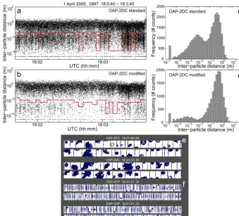
[image:5.612.67.268.66.177.2]Figure 5. Comparison of inter-particle distances measured by standard (a) and modified (b) 2DC. Red lines in (a) and (b) indicate the cut-off distanceχ∗. The distribution of the inter-particle distances for standard (c) and modified (d) probes. Examples of images obtained with an OAP-2DC at 25 µm pixel resolution (e) and an OAP-2DP at 200 µm pixel resolution (f). The measurements were conducted on 1 April during an ascent through ice cloud from approximately 4600 to 5300 m in the Ottawa region. The temperature varied from−12 to−17◦C.
χ∗=τ∗/u will be used instead of φ (1t )and τ∗, respec-tively. We will also keep using the conventional term “inter-arrival time algorithm”, although the term “inter-particle dis-tance algorithm” would be more accurate.
4.1 Description of the data set
The data used here were collected during the Airborne Icing Instrumentation Evaluation Experiment (AIIE) flight cam-paign (Korolev et al., 2011, 2013b). The analysis of the inter-particle distance is focused on the measurements of two OAP-2DCs installed side-by-side in the NRC Convair-580 aircraft. Both instruments have the same pixel reso-lution 25 µm, optics and electronics. However, one of the probes had the standard configuration, whereas the second one had modified arms with the K-tips installed (Korolev et al., 2013a). While K-tips still shatter ice particles, it has been demonstrated that they significantly mitigate the effect of shattering on ice particle measurements. Comparing mea-surements made with the standard and modified OAP-2DCs before and after applying the ITA provides an opportunity to assess the efficiency of the algorithm to successfully identify and filter out shattering artifacts. The 2-D data were
aver-aged over 5-second time intervals. For most clouds sampled during the AIIE project such averaging provided statistically significant particle numbers to estimate the functionφ (1x)
and cut-off-distanceχ∗. In the frame of this study the num-ber of bins inφ (1x) was selected to be 25. This yields a reasonable compromise between the statistical significance of number of counts in each bin and the accuracy of finding
χ∗. Usually, for a typical shape ofφ (1x), a number of par-ticle counts over 100 yielded an acceptable estimate ofχ∗
for the purposes of this work. A higher number of bins for
φ (1x)will require a higher number of counts, and therefore a longer averaging time.
4.2 Examples of the inter-particle distance distribution
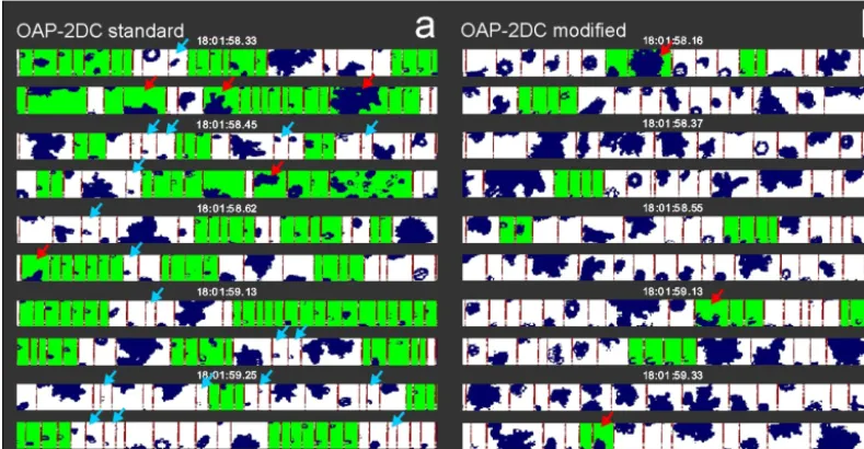
Figure 6. Examples of the results of the image rejection/acceptance processing with the inter-arrival time algorithm. The images of ice particles were simultaneously sampled by the standard (left) and modified (right) OAP-2DC during the time period shown in Fig. 5. Green backgrounds highlight the images identified by the inter-arrival time algorithm as artifacts. Images with a white background were accepted by the algorithm. As seen in (a), in some cases the standard OAP-2DC rejects large particles which appear to be intact (red arrows), at the same time it accepts particles which have the features of shattered fragments (blue arrows).
The last example demonstrates a case where shattering has a negligible effect.
4.2.1 Overlapping modes
Figure 5a and c show the time series of inter-particle dis-tances measured by the standard and modified OAP-2DC in an ice cloud. Each inter-particle distance in Fig. 5a and b is represented by a dot. The red lines indicate the cut-off-distances. As seen from these two diagrams, the density of points below the red line is greater for the standard probe (Fig. 5a) than that for the modified one (Fig. 5b). The concen-tration measured by the modified 2DC, and corrected with the help of the ITA, varied from 20 to 80 L−1. Whereas, the uncorrected concentration measured by the standard 2DC varied from 300 to 1600 L−1. After applying corrections to the standard 2DC measurements its concentration varied in the range 150 to 700 L−1. The ice particle images measured by 2DC and 2DP are presented in Fig. 5e and f. Analysis of these images shows that the ensemble of ice particles was composed of two distinct habits: large spatial dendrites with sizes up to few millimeters and transparent plates with a char-acteristic size of a few hundred micrometers. The maximum particle sizeDmaxcalculated for each averaging time interval remained approximately constant and did not exceed 5 mm.
The distributions of the inter-particle distancesφ (1x) cal-culated from the standard and modified 2DC probe data are shown in Fig. 5c and d. The inter-particle distance distribu-tion,φ (1x), for the standard 2DC displays a significant over-lap between the long and short inter-arrival modes (Fig. 5c).
This may result in rejecting intact particles along with shat-tered artifacts when1x < χ∗, and, vice versa, accepting shat-tered fragments with intact particles for1x > χ∗.
The inter-particle distance distributionφ (1x)for the mod-ified probe has a relatively small overlap between the long and short distance modes, which suggests a better separation of shattered and intact particles. The number of particles as-sociated with the short distance mode for the modified probe (Fig. 5d) is also reduced when compared to Fig. 5b. How-ever, despite the larger separation between the short and long distance modes, the ITA still identifies large particles, which appear intact, as shattered fragments (e.g., Fig. 6b).
artifacts also have a hole in the center, that is the result of the greater likelihood of shatter products entering the sam-ple volume closer to the arms and, consequently, far from the center of the depth-of-field. Further support for the assump-tion that the accepted images indicated by the blue arrows are shattered artifacts is provided by the absence of similar images recorded by the modified 2DC (Fig. 6b).
The apparently erroneous acceptance of the shattered ar-tifacts and rejection of intact images in Fig. 6a is consistent with the large overlap between the short and long distance modes indicated in Fig. 5c. This example demonstrates that the ability of the ITA to segregate shattered artifacts and in-tact particles is reduced when the short and long distance modes become less separated.
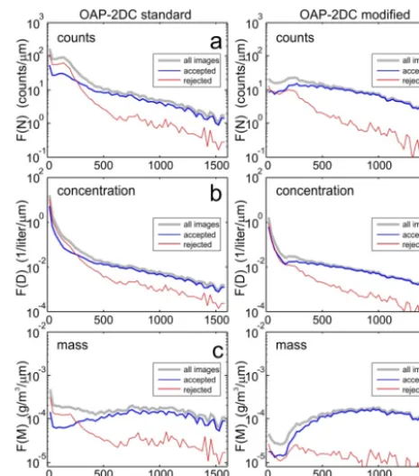
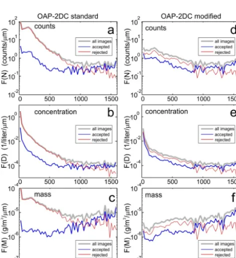
One of the important goals of filtering out shattering ar-tifacts is to obtain an accurate estimation of the PSD. Fig-ure 7 shows the distributions of particle counts, concentra-tion and mass calculated for all images before correcconcentra-tions, after corrections. These distributions were calculated for the image sizes measured along the photodiode array direction (i.e., perpendicular to the flight direction). Equivalent distri-butions are shown for the rejected images. During the im-age processing, the distribution of counts is used as a start-ing point for the followstart-ing calculations of other distributions and bulk microphysical parameters. As seen from Fig. 7a and d for both standard and modified OAP-2DCs the num-ber of small particles rejected by the inter-arrival algorithm is nearly two orders of magnitude greater than for the large par-ticles. This is consistent with the concept that shattered parti-cles are mainly composed of small fragments. Experimental studies indicate that the fragments of ice particles shattered at the aircraft speed have characteristic size from tens to hun-dreds of micrometers (Vidaurre and Hallett, 2009). There-fore, it is hypothesized that rejected particles larger than ap-proximately 1mm (Fig. 7) are likely related to the cases de-picted in Fig. 2b, d, e and f.
[image:8.612.311.544.64.328.2]It is interesting to note that for the modified probe the ITA corrected and uncorrected distributions agree to better than 10 % for particles larger 600 µm (in Fig. 7d–f). However, for the standard probe the separations between ITA corrected and uncorrected distributions remain approximately constant for D> 600 µm (Fig. 7a–c) and it varies from 20 to 30 %. Despite the rejection of a large fraction of small particles (Fig. 7b) in the modified probe, the concentration of small particles (D< 200 µm) is only reduced after correction by a factor of 2 to 3 (Fig. 7e). At the same time, the concentration of particles in the small size bins (D< 200 µm) for the stan-dard probe after ITA correction still remains higher than for the modified probe. This is consistent with the above conclu-sion that the ITA is unable to filter out all shattering artifacts. The corrected concentration of small particles (D< 200 µm) measured by the modified probe is still high. It is difficult to conclude whether these particles are real or associated with shattering artifacts, for instance due to singletons, or other mis-sizing and concentration errors.
Figure 7. Distributions of particle counts (a, d), concentration (b, e), and mass (c, f) calculated for all images (grey), and accepted (blue) and rejected (red) identified by the inter-arrival time algo-rithm. The distributions were calculated for the standard (left) and modified (right) OAP-2DCs data collected in the cloud shown in Fig. 5.
Comparisons of corrected mass distributions for standard and modified probes in Fig. 7c and f show a large difference between them forD< 500 µm. However, since large particles are the major contributors into the total mass, the discrepancy at the small size end of the PSD does not produce any signif-icant effect on the bulk IWC. Integration of the mass dis-tributions for standard and modified probes shows that IWC corrected standard is systematically higher than that for the modified OAP-2DCs. For this particular case, IWC corrected standard is approximately 20 % higher, and the mean IWC values averaged over the entire time interval is approximately 4 % higher than the modified OAP-2DC.
4.2.2 Large particles
Figure 8. Comparison of inter-particle distances measured by standard (a) and modified (b) 2DC. Red lines in (a) and (b) indicate the cut-off distanceχ∗. The distribution of the inter-particle distances for standard (c) and modified (d) probes. Examples of images obtained with an OAP-2DC at 25 µm pixel resolution (e) and an OAP-2DP at 200 µm pixel resolution (f). The measurements were conducted during on 8 April (1st flight) during descent through precipitating dendrites from approximately 1300 to 500 m in the Ottawa region. The temperature varied from−8 to−2◦C.
2DC data its concentration varied in the range 1 to 10 L−1. The appearance of the particle images measured by OAP-2DC and OAP-2DP are shown in Fig. 8e and f.
The distinctive feature of the inter-particle spatial distri-butionφ (1x) calculated for the standard OAP-2DC is that it has an exceptionally high number of counts (88 %) asso-ciated with the short distance mode. This indicates that the standard probe observed mostly shattering artifacts. In con-trast, for the modified probe the distributionφ (1x)the num-ber of counts in the short distance mode is smaller than for the long distance mode.
The results of segregating the intact particles and shattered artifacts for standard and modified OAP-2DC performed by the ITA are shown in Fig. 9. The measurements made with the standard probe are dominated by artifacts with very few accepted images (Fig. 9a). The particle imagery obtained with the modified probe is largely devoid of the small im-ages typically associated with shattered fragments (Fig. 9b). An absence of small particles in subsaturated precipitating regions is consistent with the commonly accepted concept of ice formation. It is worth noting that a few small accepted
images (indicated by the blue arrows) still appear in the stan-dard 2DC imagery in Fig. 9a. It is possible that these small images are related to single fragments as in Fig. 2c and were misidentified by the ITA as intact particles.
Despite the fact that most of the images in Fig. 9b appear to be intact dendrites, many of them were rejected. Visual inspection of the rejected images in Fig. 9b indicates that nearly all of them are partially viewed images. It is likely that the partially viewed branches of dendrites (e.g., Fig. 2e) has led to the ITA confusing the partially observed closely spaced arms of the dendrite with the shattered artifacts (Sect. 3.4).
The results shown in Fig. 9 demonstrate that even for the cases where there is a good separation of the short and long distance modes (Fig. 8c, d) the ITA still misidentifies shatter-ing artifacts and intact particles.
Figure 9. Examples of the results of the image rejection/acceptance processing with the inter-arrival time algorithm. The images of ice particles were simultaneously sampled by the standard (left) and modified (right) OAP-2DC during the time period shown in Fig. 8. A green background highlights the images identified by the inter-arrival time algorithm as artifacts. Images with a white background were accepted by the algorithm. As seen in (a), in some cases the standard OAP-2DC rejects large particles which appear to be intact (red arrows), at the same time it accepts particles which have the features of shattered fragments (blue arrows).
Figure 10. Distributions of particle counts (a, d), concentration (b, e), and mass (c, f) calculated for all images (grey), and accepted (blue) and rejected (red) identified by the inter-arrival time algo-rithm. The distributions were calculated for the standard (left) and modified (right) OAP-2DCs data collected in the cloud shown in Fig. 8.
most of the small image counts as artifacts (Fig. 10a). How-ever, the number of small images accepted for the standard probe is still greater than the modified probe (Fig. 10d). The same conclusion applies to the concentration and mass dis-tributions shown in Fig. 10b, c and Fig. 10e, f.
We note that the shape of rejected distributions for the modified probe is very similar to the shape of the uncorrected distributions (Fig. 10d, e, f). Furthermore, the distributions of the accepted and uncorrected images approach each other only for particle sizesD> 1500 µm (Fig. 10a, b, c), in con-trast to the case shown in Fig. 7. For both probes, the number of rejected large particles remains relatively large, and it is related to misidentifying large particles as shattered artifacts. 4.2.3 Small ice particles
The next example was obtained during a sampling of cirrus clouds at a temperature of−35◦C and altitude of 7500 m. The maximum size of particles varied from 200 to 400 µm, and did not exceed 500 µm. The particle concentration mea-sured by the standard and modified OAP-2DCs agreed well and varied from 20 to 180 L−1.
[image:10.612.50.287.360.619.2]Figure 11. Same as in Fig. 8. The measurements were collected on 8 April (2nd flight) in cirrus clouds at altitude 7500 m and temperature
−35◦C.
demonstrated by the small number of points that lie below the cut-off-distance line (red) in Fig. 10a and b (for which
1x < χ∗), and that Fig. 12 shows very few images identified by the ITA as artifacts.
The distributions of particle counts, concentration and mass are shown in Fig. 13. All three distributions obtained with the standard and modified probes agree well with each other. The fraction of rejected artifacts is small and for prac-tical purposes their effect on the size and mass distributions has negligible effect.
These results show that for this specific case there is not much difference between the measurement obtained by the standard and modified probes. This suggests that for the cases where the ice PSD is narrow (Dmax< 400 µm) the ef-fect of shattering on the standard OAP-2DC measurements is quite small and can be neglected. This finding also im-plies that there exists a threshold size below which shatter-ing of ice crystals does not produce any significant effect on measurements. This will likely vary according to instru-mental and microphysical characteristics. Of course, even though the probes agree for this case, problems relating to mis-sizing and concentration errors for particles smaller than
∼100 microns still exist (Korolev et al., 1998; Strapp et al., 2001).
4.3 Statistical characteristics of inter-particle distances in shattering events
Figures 5a, b, 8a, b and 11a, b contain a plethora of informa-tion about the statistical characteristics of shattering events and their effect on ice particle measurements. This data can also be used in the development of future algorithms for the data processing and numerical simulations of the shattering effects. In this section some of the statistical characteristics of shattering processes will be investigated and compared with microphysical metrics.
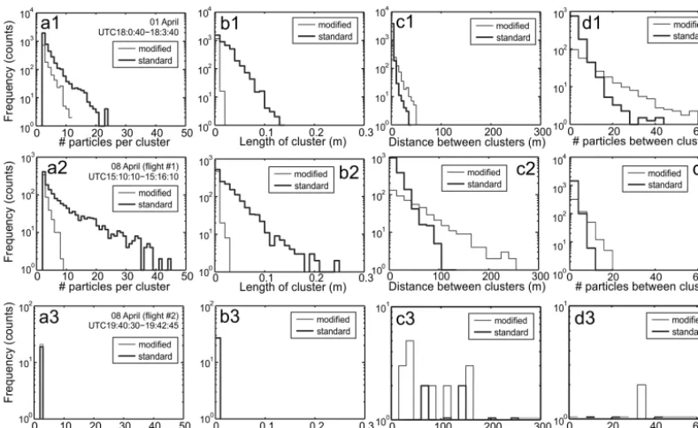
Figure 14 shows distributions of the number of parti-cles Ns within each shattering event (a1–a3), distributions of the length of spatial clusters along the flight directionLs (b1–b3), distributions of distances between shattering events
Li (c1–c3), and the number of particles between shattering eventsNi (d1–d3). These distributions were calculated for the cloud regions shown in Figs. 5, 8 and 11.
Figure 12. Same as in Fig. 6. The measurements of the images were obtained during the time period shown in Fig. 11.
Figure 13. Distributions of particle counts (a, d), concentration (b, e), and mass (c, f) calculated for all images (grey), and accepted (blue) and rejected (red) identified by the inter-arrival time algo-rithm. The distributions were calculated for the standard (left) and modified (right) OAP-2DCs data collected in the cloud shown in Fig. 11.
depends on the presence of large particles in the size distri-bution and is correlated withDmaxsuch that increasingDmax leads to a shallower slope for f (Ns): Figure 14a2 displays
the shallowest slope inf (Ns)for the case with the greater Dmax.
The distribution of f (Ns)monotonically increases with decreasingNs, having a maximum for events with two shat-tered fragments. Extrapolatingf (Ns)towards 1, i.e., shat-tering events with one particle, suggests that the number of singletons may be quite high. Existence of single particle shattering events presents a principal limitation of the inter-arrival algorithm, since such particles cannot be unambigu-ously identified as artifacts merely based on the analysis of
1x.
The maximum number of the shattered fragments in a shattering event measured by the standard OAP-2DC dur-ing the AIIE project reached 60. Whereas for the modified probe, the maximum number of fragments for this data set was found to be 14. Figure 14a1 and a2 also demonstrate that the modified OAP-2DC on average has a smaller number of fragments per shattering event, and therefore the antishatter-ing tips can efficiently mitigate shatterantishatter-ing.
The density function of the length of spatial clusters of shattered fragmentf (Ls)can also be well approximated by an exponential function (Fig. 14b1, b2). Clusters with a short length have the highest probability and they are associated with two-particle shattering events. The spatial length of the shattering clusters is presented by a cascade of scales rang-ing from zero to tens of centimeters. The maximum length of the shattered clusters measured by the standard and modi-fied OAP-2DCs during the AIIE project reached 30 and 3 cm, respectively.
[image:12.612.50.288.317.578.2]Figure 14. Distributions of number of particles per shattering event (a1, a2, a3), length of the clusters of shattered artifacts along the flight direction (b1, b2, b3), distance between the clusters with shattered fragments (c1, c2, c3), number of intact particles between shattered events (d1, d2, d3) calculated for the cases shown in Fig. 5 (top row), Fig. 8 (middle row) and Fig. 11 (bottom row), respectively.
in Fig. 14c3 has the highest total concentration of ice par-ticles. However, only 0.7 % (∼30 counts) of them generate shattering events. As a result thef (Li)in Fig. 14c3 has a sta-tistically insignificant distribution. As in the previous cases
f (Li)can be well approximated by an exponential function and the characteristic value ofLi for modified OAP-2DC is larger than that for the standard probe (Fig. 14c1, c2).
The behavior of the functionf (Ni)in Fig. 14d1–d3 is very similar to that off (Li)(Fig. 14c1, c2, c3). For the case de-picted in Fig. 14d3 the low number of shattering events mean that most of the counts are outside of the scale.
Figure 15 shows the distributions of cut-off distances,
f (χ∗), for the standard and modified OAP-2DCs averaged over all ice clouds sampled during the AIIE project. Because the value ofχ∗depends of the size distribution of ice parti-cles and their habits, the shape of the distribution,f (χ∗), will be determined by a combination of cloud characteristics, air-craft and instrument properties. However, the distributions of
f (χ∗)in Fig. 15 allow a few conclusions to be made. Firstly, for the OAP-2DCχ∗ can vary from tens of micrometers to approximately one meter. Secondly, the standard probe χst∗
has a mode at approximately 10 cm, whereas the modified probeχmdf∗ has a mode at approximately 2 cm.
4.4 Effect of particle sizes
The effect of particle sizes on shattering is demonstrated in Fig. 16 which shows the maximum number of fragments per shattering event Nsmax vs. Dmax for standard and modified
probes. TheNsmaxandDmaxwere calculated for each 5 s av-eraging interval for the entire AIIE project. Figure 16a shows that forDmax< 15 mm,Nsmaxcorrelates well withDmaxand therefore the dependenceNsmax(Dmax)can be parameterized with a linear function (Fig. 16a). However, for the modified probe the correlation coefficient betweenNsmax and Dmax is low (0.57) and theNsmax(Dmax)saturates atNsmax ∼15 whenDmax> 5 mm (Fig. 16b).
Figure 17 shows the maximum length of shattering clus-tersLsmaxvs.Dmaxfor standard and modified probes. Simi-lar to the case in Fig. 16,Lsmax andDmaxwere calculated for each 5 s averaging interval. A relatively high correla-tion coefficient betweenLsmaxandDmax(0.78) for the stan-dard probe allows linear parameterization of Lsmax(Dmax) (Fig. 17a). The correlation coefficient between Lsmax and Dmaxfor the modified probe is quite low (0.29), butLsmax is never longer than 3 cm for allDmaxencountered.
The nearly linear increase ofNsmax andLsmax with the increase ofDmaxfor the standard probe (Figs. 16a, 17a) in-dicates a strong dependence of particle size on particle shat-tering.
5 Monte Carlo simulation of inter-particle distance function
simula-Figure 15. Distribution of cut-off distancesχ∗for standard (a) and modified (b) OAP-2DCs averaged over all ice clouds sampled dur-ing the AIIE project.
tions were used to understand the influence of various param-eters on the shape of the inter-particle distance distribution,
φ (1x).
For each simulation, two fluxes of particles with the same concentrationn0are assumed to interact with the probe. The first flux represents intact particles and passes through the sample areaS0of the probe. The second flux represents the shattered particles and passes through a “shattering” area for the probe,Ssh, rebounds and subsequently passes throughS0. After passing though Ssh, a particle breaks down into Nsh fragments.
The inter-particle distance between the intact particles was simulated assuming a Poisson distribution by combining a random number generator with an exponential distribution with mean distance χ¯0=nS0
0. The inter-particle distance be-tween the shattering events was also simulated using an ex-ponential distribution with mean distance χ¯ev=Snsh0. Based on the results obtained in Sect. 4.3, the number of shattered fragments was simulated by a random number generator with exponential distribution with averageN¯sh. The distance be-tween the shattered fragments in each shattered event was also simulated by the exponential distribution with average
¯
χsh= ¯ Ls
¯
Nsh, where
¯
[image:14.612.83.250.67.338.2]Lsis the average distance of the cluster of shattered fragments. After sorting arrival times, the two flows were merged together to form a time series of intact particles mixed with the shattering artifacts.
Figure 16. Scatter diagram of the maximum number of shattered fragments per event vs. maximum particle sizes for standard (a) and modified (b) OAP-2DCs for all ice clouds sampled during the AIIE project.
The modeling results presented below were performed for
S0=50 mm2,Ssh=5 mm2,L¯s=1 cm andN¯sh=5. The par-ticle size distribution was assumed to be monodisperse.
Figure 18 shows the modeled distributions of the inter-particle distances for intact inter-particles only, φi(1x) (blue), shattered particles only,φs(1x)(red), and all particles that passed through the sample volume,φ (1x)(black). The dis-tribution φi(1x) represents the Poisson process and has a single mode, whereasφs(1x)has two modes. The long dis-tance mode in φs(1x) is determined by the characteristic distance between the shattered eventsχ¯ev, whereas the short distance mode is associated with the characteristic distances between the shattered fragmentsχ¯sh, which passed through the sample volume. The long distance mode inφs(1x)also includes single particle shattering events. This is what we see for the long mode of the red line (rebounders/singletons) and the blue line. Both of these are continuous processes, whereas the shorter shattering mode is intermittent condi-tional on a collision occurring in the shattering volume. It is important to mention that the inter-particle distribution
[image:14.612.343.512.68.332.2]Figure 17. Scatter diagram of the length of clusters of shattered fragments vs. maximum particle sizes for standard (a) and modified (b) OAP-2DCs for all ice clouds sampled during the AIIE project.
Figure 19 shows four distributions φ (1x) calculated for the particle concentrations 1, 10, 100, and 1000 L−1. Fig-ure 19 shows that the long distance mode approaches the short distance mode, when the particle concentrationn0 in-creases. However, the short distance mode is insensitive to the changes of the particle concentration, and it remains at the same position, when n0 increases (Fig. 19a, b, c). The location of the cut-off-distanceχ∗appears insensitive to the changes inn0, remaining approximately constant.
For increasingn0 the reduced separation of the long and short distance mode results in an increased overlap of the dis-tributions associated with these modes. As described above, increasing the overlap of these distributions reduces the effi-ciency of the ITA to segregate intact particles and shattered artifacts. At high concentrations the short and long distance modes merge, resulting in the vanishing of the inter-modal minimum. At that stage the ITA becomes much less efficient or even disabled (e.g., Fig. 19d).
In the above simulations the particle size distribution was assumed to be monodisperse. One of the consequences of this assumption is that all of the particles possessed the same shattering efficiency andN¯shremains the same for all parti-cles. In reality, particle sizes in natural clouds are represented by broad distributions. As indicated above,N¯shdepends on particle sizes and that for small particles with D< 400 µm
¯
Nsh→0. Therefore, the concentrationn0 should be
inter-Figure 18. Results of Monte Carlo simulations of the distribution of inter-particle distanceφ (1x)for intact particles (blue), shattered particles (red), and all particles passed through the sample volume (black). The calculations were conducted for particle concentration n0=100 L−1.
preted as a concentration of the particle’s contribution in the effect of shattering, but not as a total concentration, which included small ice particles which do not affect shattering. For simplicity, the effect of the particle size distribution was not included in the simulation. It should be noted that the threshold 400 µm refers to OAP-2DC. Probes with different pixel resolution, response time, and inlet configuration have different threshold sizes below which the effect of shattering becomes insignificant.
[image:15.612.82.254.68.339.2]ex-Figure 19. Results of Monte Carlo simulations of the distribution of inter-arrival timeφ (1x)for different particle concentrations (a) 1 L−1; (b) 10 L−1; (c) 100 L−1; (d) 1000 L−1.
plained by the fact that the antishattering tips have a signifi-cantly reduced shattering area compared to the standard tips.
6 Conclusions
Based on the analysis of data obtained with standard and modified OAP 2DC probes in a variety of ice cloud con-ditions and Monte Carlo simulations, the following conclu-sions have been obtained:
1. The inter-arrival time algorithm cannot segregate all shattering artifacts from the intact particles in principle. These limitations are imposed by the Poisson statistics of particle spatial distribution. It was demonstrated that the short inter-arrival times are not necessarily associ-ated with shattering artifacts, and that shattered artifacts are not constrained to exhibit short inter-arrival times. In order to mitigate the effect of shattering, the inter-arrival time algorithm should be used together with other means, such as antishattering tips and special al-gorithms to improve its performance (e.g., reacceptance of intact particles, corrections for accepted singletons, etc.).
2. The inter-arrival time algorithm has a range of condi-tions when short and long inter-arrival modes are well separated and it can effectively segregate shattered arti-facts and intact particles (e.g., low concentration). 3. The inter-arrival time algorithm has a number of
limi-tations which under certain circumstances may signifi-cantly degrade its performance or even disable it. Such cases are relevant to the clouds with high particle con-centration, when the spatial separation between shat-tered fragments1xsbecomes comparable with the dis-tance between intact particles1xi, i.e.,1xs∼1xi. For mixed-phase clouds it may not be possible to use the inter-arrival time algorithm with probes that have a fine pixel resolution.
4. It was found that in clouds with particles with
Dmax< 400 µm the effect of shattering on measurements of the standard OAP-2DC can be neglected.
5. The inter-arrival distance and number of registered shat-tered artifacts is well represented by an exponential function. The slope of the distribution is a function of the characteristic particle size. The number of shattered fragments correlates with particle size.
6. The results on the statistics of shattering events open the door for a statistical simulation to study the effect of shattering on measurements. These studies could po-tentially be useful not only for developing correction al-gorithms for historical data sets but also for developing recommendations on how to design probes in the future to best accommodate the ITA.
[image:16.612.83.252.64.549.2]Edited by: A. Lambert
References
Baker, B., Mo, Q., Lawson, R. P., O’Connor, D., and Korolev, A.: The Effects of Precipitation on Cloud Droplet Measurement De-vices, J. Atmos. Ocean. Tech., 7 1404–1409, 2009.
Baumgardner, L., Avallone, A., Bansemer, S., Borrmann, P., Brown, U., Bundke, P., Chuang, Y., Cziczo, D., Field, P., Gallagher, M., Gayet, J.-F., Heymsfield, A., Korolev, A., Krämer, M., McFar-quhar, G., Mertes, S., Möhler, O., Lance, S., Lawson, P., Pet-ters, M. D., Pratt, K., Roberts, G., Rogers, D., Stetzer, O., Stith, J., Strapp, W., Twohy, C., and Wendisch, M.: In Situ, Airborne Instrumentation: Addressing and Solving Measurement Prob-lems in Ice Clouds, B. Am. Meteorol. Soc., 93, ES29–ES34, doi:10.1175/BAMS-D-11-00123.1, 2012.
Cooper, W. A.: Cloud physics investigation by the University of Wyoming in HIPLEX 1977, Bureau of Reclamation Rep, AS, 119, 321 pp., 1977.
Field, P. R., Wood, R., Brown, P. R. A., Kaye, P. H., Hirst, E., Green-away, R., and Smith, J. A.: Ice particle inter-arrival times mea-sured with a Fast FSSP, J. Atmos. Ocean. Tech., 20, 249–261, 2003.
J. Atmos. Ocean. Tech., 24, 376–389, 2007.
Korolev A. V., Strapp, J. W., and Isaac, G. A.: Evaluation of accu-racy of PMS Optical Array Probes, J. Atmos. Ocean. Tech., 15, 708–720, 1998.
Korolev, A., Emery, E. F., Strapp, J. W., Cober, S. G., Isaac, G. A., Wasey, M., and Marcotte, D.: Small ice particles in tropospheric clouds: fact or artifact? Airborne Icing Instrumentation Evalua-tion Experiment, B. Am. Meteorol. Soc., 92, 967–973, 2011. Korolev, A., Emery, E., and Creelman, K.: Modification and tests of
particle probe tips to mitigate effects of ice shattering, J. Atmos. Ocean. Tech., 30, 690–708, 2013a.
Korolev, A. V., Emery, E. F., Strapp, J. W., Cober, S. G., and Isaac, G. A.: Quantification of the effects of shattering on airborne ice particle measurements, J. Atmos. Ocean. Tech., 30, 2527–2553, 2013b.
Lawson, R. P.: Effects of ice particles shattering on the 2D-S probe, Atmos. Meas. Tech., 4, 1361–1381, doi:10.5194/amt-4-1361-2011, 2011.
Strapp, J. W., Albers, F., Reuter, A., Korolev, A. V., Maixner, U., Rashke, E., and Vukovic, Z.: Laboratory Measurements of the Response of a PMS OAP-2DC, J. Atmos. Ocean. Tech., 18, 1150–1170, 2001.