Thesis by
Malcolm B. Gray
far Partial Fulfilment of the Requirements for the Degree of
Doctor of Philosophy
Australian National University Canberra,
Australian Capital Territory
For providing vision, inspiration and tremendous patience, I thank my thesis supervisors Hans-A. Bachor and David E. McClelland. Without their leadership and overall sense of direction this thesis would not have been possible.
For his enthusiasm in both theoretical analysis and experiment, I thank Andrew J. Stevenson.
For his patience, laboratory expertise and attention to detail, I thank Charles C. Harb.
I am grateful to the entire workshop team whose technical support has been invaluable over the past four years. Particularly I thank Brett Brown, Alex Eades, David Cooper and Paul Tant.
This thesis is an account of research undertaken in the Department of Physics and Theoretical Physics, at the Australian National University between February 1991 and December 1994 while I was enrolled for the degree of Doctor of Philosophy.
This research was supervised by Dr Hans-A. Bachor and Dr David E. McClelland, but unless otherwise indicated, the work presented herein is my own.
None of the work presented here has ever been submitted for any degree at this or any other institution of learning.
Malcolm Bruce Gray
A small bench top interferometer, built to study modulation interferometry is described. A number of different interferometer configurations are trialed, all using a continuos wave, Nd:YAG laser. The ability of these configurations to operate at the shot noise limit is documented and technical noise sources that detract from this limit are investigated.
The frequency and intensity noise properties of the Nd:YAG laser, used throughout this work, are documented. It is shown that the free running laser has considerable frequency noise structure from DC to approximately 100kHz. The effects of this frequency noise on interferometry are documented and means of overcoming these problems discussed.
The free running laser is shown to exhibit strong intensity noise structure associated with the resonant relaxation oscillation present in the lasing crystal. The resonant relaxation oscillation is modelled by a noise-driven second order system. This description is used to design an intensity stabilisation servo to suppress the free running laser noise. The performance of the stabilisation system is documented and its ability to suppress laser intensity noise by up to 35dB across a wide bandwidth is demonstrated.
A simple scalar theory, to describe modulation interferometry is developed. All necessary non-ideal parameters are included and accurate predictions of practical interferometer sensitivity are made. The theory is used to analyse the performance of all interferometers tested here.
Bench top interferometer experiments are performed for direct detection, internal modulation, external modulation and power recycling interferometer configurations. The shot noise sensitivity of each configuration is measured and excellent agreement with theory is achieved.
An application for the direct detection interferometer is demonstrated; non- invasive shot noise limited RF electric field measurements. Several circuit boards are mapped using this device and the results presented.
Non-stationary shot noise in internal m odulation interferometers is investigated. Using a large modulation depth and high fringe visibility interferometer, approximately 4.8dB of noise variation dependent on the demodulation phase is achieved. Non-stationary shot noise is shown to cause excess noise (1.7dB) in the signal quadrature, leading to shot noise limited sensitivity of
V(
3/2) worse than direct detection.A complex modulation-demodulation system is then implemented using both the first and third harmonic. The addition of the third harmonic is shown to introduce correlated shot noise that can be used to reduce the excess 1.7dB non- stationary shot noise occurring in the signal quadrature.
Acknowledgments iii
Abstract v
Chapter 1 Introduction 1
Chapter 2 Basic Physics of Quantum Noise Limited Interferometry 9
2.1 Gaussian beams in interferometers. 10
2.2 Beam splitter operation. 10
2.3 Basic interferometer types. 11
2.4 Shot noise and quantum efficiency in optical
measurements. 19
2.5 Electronic mixer operation. 21
2.6 The Pound-Drever error signal. 23
2.7 Spectrum Analyser operation. 24
2.8 Basic servo theory. 28
Chapter 3 Practical Aspects of Photodetectors and Lasers 31
3.0 Perspective. 32
3.1 Photodetector performance. 33
3.2 Laser intensity noise characterisation. 34
3.3 Stabilisation of a Nd:YAG laser. 42
3.4 Laser frequency noise characterisation. 58
3.5 Conclusion to chapter three. 68
4.0 Perspective 71
4.1 Derivation of direct detection theory. 72
4.2 Implications of th e o ry . 75
4.3 Direct detection experiments. 79
4.4 Electric field m apping using direct detection
interferometry. 87
4.5 Conclusion to chapter four. 90
Chapter 5 Internal Modulation Interferometry 93
5.0 Perspective. 94
5.1 Derivation of internal m odulation theory. 95
5.2 Experimental description. 108
5.3 Non-stationary shot noise in internal m odulation
interferometers. 114
5.4 Conclusion to chapter five. 127
Chapter 6 External Modulation Interferometry 129
6.0 Perspective. 130
6.1 External m odulation interferometry:
A generic model. 131
6.2 Experimental configuration. 143
6.3 Experimental results. 148
6.4 Conclusion to chapter six. 161
7.0 I Perspective. 164 7.1 A simple theory to describe power recycling. 165
7.2 Optical and electronic configuration. 169
7.3 Experimental results of power recycling. 176
7.4 Conclusion to chapter seven. 180
Chapter 8. Summary and Recommendations for further work 183
8.0 Summary 183
8.1 Recommendations 186
Cited References 189
Appendix A Photodetector design and development. 195
Appendix B Phase locked loop design and performance. 209
Chapter 1
Introduction
A brief overview
A fundamental limitation in the measurement of any real quantity is set by the Heisenberg uncertainty principle1. The object being measured exhibits quantum mechanical fluctuations that ultimately limit the sensitivity of the measurement that can be made in a finite time, commonly referred to as the
"standard quantum limit". Detailed quantum mechanical analysis of optical interferom eters has shown that using large laser powers, optical interferometers can reach the standard quantum limit2'3. Two physical mechanisms produce the noise responsible for this limit in interferometers: photon counting errors and fluctuating radiation pressure force on the interferometer mirrors. Photon counting errors scale inversely with laser power while fluctuating radiation pressure force scales proportional to optical power. When the two noise sources are equal, the standard quantum limit is achieved. Practical interferometer lasers are however several orders of magnitude too weak to reach this limit2. The limiting source of quantum noise in realistic interferometers is therefore due to photon counting error alone (commonly termed the "shot noise limit ").
Using quantum mechanical operator theory, the sources of quantum noise, in an interferometer measurement can be identified4. The same theoretical approach can also be utilised to demonstrate the advantages of non-classical light states or "squeezed light"5. It has been shown that by using squeezed light sources, rather than coherent light, it is possible to reach the quantum limit at lower laser powers. In principle, one can trade off laser power for the degree of squeezing of the source2'6.
The optical power currently available for interferometric light sources allows us to discard the effects of radiation pressure. Under this 'Tow power" limit, quantum noise limited interferometer sensitivity is proportional to l/V(optical power). Hence high sensitivity interferometers require large laser power9'10'11. For example the estimated shot noise limited strain sensitivity of the VIRGO project of 10'22 A1/1/VHz requires a circulating interferometer power of ~ 1000 watts.
While the shot noise limit sets a practical constraint to interferometer sensitivity, a number of technical noise sources have the potential to seriously degrade this limit in a practical instrument.
Vibrational noise, due to seismic activity, acoustic pick up or thermal excitation are present in all optical components. As it is not possible to discriminate between mirror vibrations due to noise sources and that due to "signals", the presence of vibrational noise limits the achievable sensitivity.
An ideal interferometer is, in principle, immune to both laser intensity and frequency noise. However this is true only for perfectly matched interferometer arms12. Small deviations in the arm length cause frequency noise to produce a phase noise at the beam splitter, producing noise in the signal spectrum. Likewise, an intensity mismatch in the interferometer arms couples fluctuating power to the detectors and the signal spectrum.
All the above noise sources either shake interferometer mirrors directly (vibrational noise) producing an RMS Al or can be modelled as producing an equivalent Al (laser noise etc). The combination of all these technical noise sources produces a sensitivity limit that can be expressed in Al (m/VHz). This limit is many orders of magnitude larger than the standard quantum limit and usually larger than the shot noise limit for moderate signal frequencies (acoustic frequency band).
Fortunately a number of techniques are available to either reduce the size of these technical noise sources directly or reduce their coupling into the signal spectrum.
frequency acoustic noise. Evacuating the interferometer removes direct acoustic pick up.
Thermal noise, an inevitable consequence of the fluctuation-dissipation theorem15, is present in all mechanical interferometer components. By making all the relevant optical components exhibit large mechanical Q's, the thermal energy can be restricted to specific frequency bands, minimising the impact on the signal spectrum15.
Active feedback control can be used to greatly reduce laser frequency noise by locking the instantaneous laser frequency to an acoustically isolated, Fabry- Perot reference cavity16'17. Laser intensity noise can also be dramatically reduced by using a high-gain servo system18'19'20.
Signal modulation/demodulation can be utilised to reduce the noise coupled into the signal spectrum21. Optical phase modulation/demodulation has been shown to give up to ~ 60dB of isolation from common mode interferometer noise22.
For high sensitivity applications, passive isolation, active feedback stabilisation and signal modulation are all required in order to reach the design goals9'10'11. Once technical noise sources have been reduced to the point where sensitivity is limited only by shot noise , several sensitivity enhancing techniques can be used to improve the resulting shot noise limited sensitivity:
Power recycling23 can be used to increase the circulating interferometer power and hence imitate a larger laser power (with a corresponding improvement in the shot noise limited sensitivity). When a Michelson interferometer is operated so that the output port is on a dark fringe, the incident light is directed back to the laser. Placing a partially reflecting mirror between the laser and the interferometer then turns the interferometer into a resonant cavity. The circulating power in the interferometer can be enhanced by up to l/(loss per pass)24 and the shot noise limited sensitivity can be improved by up to V(loss per pass).
be resonant in. Dual recycling therefore, involves a trade off between sensitivity and signal frequency response27.
Motivation
The Australian Consortium for Laser Interferometer Gravitational Wave Detection is currently working towards building a large scale gravity wave interferometer28. In order to build up local expertise, the consortium is funding work in three major areas: laser interferometer techniques, mechanical isolation systems and laser development.
The work reported in this thesis is the first sequence of experiments performed under the consortium direction in order to develop laser interferometer techniques. This thesis therefore fulfils two main aims: it lays the ground work for more complex and realistic experimental prototypes to be developed within the consortium and, it develops local knowledge towards designing and building a large scale interferometer in Australia.
Finally, the interferometry experiments undertaken here have another purpose; they serve to demonstrate the applicability of techniques developed in the Gravity Wave community to a broad scientific audience.
This thesis
This thesis focuses on investigating modulation interferometry techniques on a laboratory bench top interferometer. A simple descriptive theory of modulation interferometry is developed. We treat quantum noise (shot noise) as a purely phenomenological effect occurring at the photodetector. This approach can be justified by noting that here we are considering only "classical " states of light and linear optical operations. Ultimately, the justification for using this simple "classical" approach is that the results are in agreement with the full quantum treatment given by Caves2.
variables are excluded in order to maintain clarity. The theory developed in this thesis therefore includes macroscopic variables such as e (the electronic noise ratio), a (the power split off ratio for external modulation), modulation depth 0m and V (the fringe visibility). Second order variables, such as beam pointing error, mode mismatch and detector surface area responsivity variation, are excluded to maintain the clarity and transparency of the theory. The effect of critical experimental variables, in the theory of this thesis, is clear and the trade-offs necessary for optimum interferometer sensitivity are easily developed.
We derive the signal-to-noise ratio as a function of all the experimental variables included in the model and so we can directly compare, non-ideal experimental results with our theoretical predictions.
A series of modulation experiments are performed starting with direct detection. We investigate increasingly complex systems culminating in the final interferometer configuration explored here; power recycled with external modulation. Quantitative signal-to-noise analysis is performed at each stage and comparison to theory is made.
Solid state diode-pumped, monolithic, Nd:YAG ring lasers are used throughout this thesis. They have a number of significant advantages compared with gas lasers; they are intrinsically more stable29'18, reliable11 and efficient30. Power limitations with diode-pumped, solid state lasers has limited their use in the past, however ongoing research programs are overcoming this drawback31'32.
Considerable effort is directed at characterising the lasers used and improving their noise performance. Both intensity and frequency noise characteristics are determined and an intensity noise stabilisation experiment is performed.
Outline
This thesis is divided into eight chapters covering the bench top interferometry and associated experiments performed over the past four years.
For example, the basic phase response of Michelson, Mach-Zehnder and Fabry- Perot interferometers are derived as well as a brief discussion on the operation of a double balanced mixer.
Chapter three describes practical aspects of both photodetectors and lasers. The performance of the three photodetectors, designed for this thesis, is documented. The intensity noise performance of a diode-pumped Nd:YAG laser is documented and an experiment to suppress this noise by electro-optic feedback, is presented.
Two tests of the frequency noise of a diode-pumped, Nd:YAG laser are then presented and the implications of the noise structure are discussed. The frequency noise results derived in this chapter (for a Lightwave 120 laser) are used several times in later chapters, to explain the presence of frequency noise in the signal spectrum.
Chapter four presents the theory and experimental data concerning direct detection interferometry. The frequency limitations of direct detection are presented and compared to the intensity noise spectrum of the laser (documented in chapter three).
A direct detection polarimeter for sensing RF electric field distributions is described. Several experimental maps of electric field distributions are presented which demonstrate the usefulness of this device.
Internal modulation interferometry, both theory and experiment are covered in chapter five. The theory developed describes both the limiting performance of internal modulation as well as the effects of typical non-ideal parameters (eg electronic noise, poor fringe visibility etc). A comparison between the predicted sensitivity and achieved sensitivity is given, showing excellent agreement.
External modulation interferometry theory is developed in chapter six. This is compared to experiments in both the large and small signal limits. Once again, excellent agreement between theory and experiment is found.
The cause of anomalous noise structure below 100kHz is investigated and found to be due to frequency noise of the laser. The anomalous noise features evident in the external modulation interferometer signal spectrum are in close agreement with the frequency noise spectrum measured in chapter three.
Chapter seven expands the external modulation theory to include power recycling. A power recycling experiment is performed and compared with the theory. Broad agreement is reached, however technical noise in the baseband signal spectrum prevented the measurement from being shot noise limited.
The noise implications of scattered light at the signal photodetectors are experimentally demonstrated. The origins of this noise are developed and means of overcoming the problem are discussed.
Basic Physics of Quantum Noise Limited
Interferometry
The purpose of this chapter is to provide the physical and mathematical background that will be required in later chapters. The topics covered here may appear to be disparate but will be seen to be essential in developing the analysis of future chapters.
The chapter starts with a description of Gaussian beams in free space and explains why our analysis can assume perfect Gaussian mode matching on all beams. We then define a convention for determining the intensity of a light beam based on an electric field formalism that will be used throughout this thesis.
The phase properties of a beam splitter, consistent with power conservation, are developed. We then have sufficient analytic tools to describe a generic interferometer. We analyse both Michelson and Mach-Zehnder interferometers in order to derive the output intensity as a function of optical phase before considering the frequency and phase response of a Fabry-Perot interferometer.
We define the basic expressions for shot noise and quantum efficiency as well as Noise Equivalent Power (NEP) and Relative Intensity Noise (RIN) for a shot noise limited beam.
The operation of a double balanced mixer is then described, followed by an explanation of the Pound-Drever error signal generation.
2.1 Gaussian beams in interferometers.
Gaussian modes of radiation provide a useful, although not exclusive, complete set to describe all optical propagation in free space. They can be derived directly from Maxwells equations33 and provide a natural basis for the study of lasers and interferometry.
The propagation of Gaussian modes through an interferometer can be described by the usual complex "q" parameter33. The type of analysis carried out in this thesis assumes that all Gaussian beams propagate undeformed and interfere with complete efficiency when merged with other Gaussian beams. Gross interference problems, via mode distortion, mode mismatch or beam size difference are treated as an experimental problem that can usually be rectified with careful alignment and component positioning. The effects of finite fringe visibility can be treated in our scalar analysis via differential loss and amplitude mismatch alone.
We are therefore free to consider radiation fields inside interferometers as defined by a single scalar, complex variable "E". By assigning appropriate amplitude and phase changes to the individual fields as they propagate through an interferometer, all relevant behaviour can be modelled and predicted.
As all optical measurements involved w ith this thesis are intensity measurements, it is convenient to define the free space electric field such that:
E E* = Popt (2.01)
where Popt is the total optical power that the complete mode described by "E" is capable of delivering across some interface.
2.2 Beam splitter operation.
Figure 2.1: Electric field formalism for a symmetric beam splitter.
Incident Electric
F-i e l d
Reflected Electric Field
E/V2
Transmitted Electric Field
e i 7 r / 2 e / V 2
r
2.3 Basic interferom eter types.
Three basic interferom eter configurations will be studied in this thesis, they are: the M ichelson interferom eter, the M ach-Zehnder and the Fabry-Perot interferom eter. The basic phase and intensity response of all three types will now be derived for later use.
The Michelson Interferometer
The basic layout of the Michelson interferometer is show n in Fig (2.2). Let Eine be the electric field incident on the interferometer. Following the beam splitter formalism outlined in section 2.2, the electric field incident on the detector is:
w here a and b are the pow er reflectivities of the end m irrors and 0ab is the total phase difference betw een the two arms at their recom bination, excluding the phase shifts of the beam splitter. The electric field returning to the laser is given by:
Edet = { Va e ( ^ 2+0ab) Eine + Vb e^/2 Eine}/ 2 (2.02)
^return — { Va 0(itt+6ab) E ^ H - Vb E ^ c } / 2 (2.03)
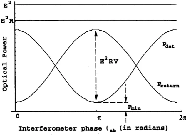
P d et = l^inc^ R / 2 ( 1 "*■ V COS0ab)
Pretum = Ejnc2 R /2 ( 1 - V COs6ab) (2.04)
w here R = (a + b )/2 is the m ean m irror reflectivity and V = 1/r (ab)1' 2 is the
fringe visibility of the interferom eter. Both P d e t and P re turn are plotted as a
function of interferometer phase in Fig (2.3) for R =0.85 and V = 0.8.
As can be seen for non-ideal values of R and V (R and V less than 1) the effective input pow er is no longer EinC2 but E^c2 R and the fringe height is then given by the effective input pow er m ultiplied by the fringe visibility E in C2 R V.
[image:19.550.113.413.425.674.2]The dark fringe optical transm ission through the interferom eter is in general, non zero and given by Pmin = EinC2 R /2 (1 - V)
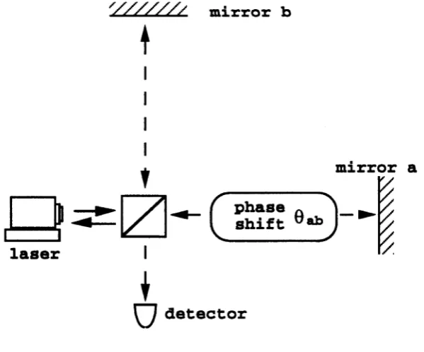
Figure 2.2: The Michelson interferometer. Note that 0ab is the phase shift incurred after a double pass of arm a with respect to the phase shift incurred after a double pass of arm b.
' / / / / / / /
\
I
I I
I
mirror b
f
phase l shiftmirror a
laser
♦
Figure 2.3: Detector optical power versus interferometer phase 0ab
(in radians) Interferometer phase (
The Mach-Zehnder Interferometer
The Mach-Zehnder interferometer is another amplitude splitting interferometer and its general form is outlined in Fig (2.4) Once again, let E^c be the electric field incident on the interferometer. Propagating the electric field through both arms of the interferometer, with the beam splitter formalism outlined in section 2.2 gives the two output fields:
Ei
= { Va
e ( i* /2 + 9 a b) Ejnc +Vbe
^ 2
Etac}/ 2E2 = {Va e i ö a b Einc +
Vb
e>* E™ }/2 (2.05)Using equation (2.01) to determine the optical power at detectors 1 and 2 gives: Pi = Eine2 (1 + V cos9ab) R/2
P2 = Eine2 ( 1 - V COS0ab) R /2 (2.06)
Figure 2.4: The Mach-Zehnder interferometer
mirror b
laser
mirror
s:
I
f detector 1
O
t
U
detector 2The Fabry-Perot Interferometer
Unlike the Michelson or Mach-Zehnder interferometers, the Fabry-Perot interferometer combines an infinite sum of related electric fields and is therefore capable of producing strong resonant behaviour. A simplified schematic of a Fabry-Perot interferometer is shown in Fig (2.5), where it is assumed that the interferometer is loss less (no intra-cavity elements) apart from the input and output coupling mirrors.
The following analysis derives the basic relationships between all the electric field variables and is based on a derivation given by Siegman34.
Figure 2.5: Schematic of a Fabry-Perot interferometer.
circ trans
ref 1
Using the beam splitter formalism of section 2.2 for both the input and o u tput m irrors and assuming that EinC is the only incident field on the interferometer:
Ecirc = i V(l-a) + V(a b) e j (-2®L/c) Ecirc (2.07)
w here L is the interferometer length , a and b are the respective m irror pow er
reflectivities, co is the frequency of the incident light field and V(l-a) is the electric field transmissivity of m irror a. Equation (2.07) can be reorganised to
give:
Ecirc / Eine = i V(l-a) /{ I -V(a b) e* (-2ö»L/c) } (2.08)
The transm itted electric field is directly proportional to the circulating cavity field. Taking into account the transmissivity of m irror b and the phase shift of the circulating field as it propagates from m irror a to m irror b (the circulating cavity field is arbitrarily defined at m irror a) the transm itted electric field can be w ritten as:
E lrans = i V(l-b) Ecirc e 1 (2.09)
As a function of the incident electric field, the transm itted electric field is:
Etrans /E in e = -V(l-a)V(l-b) e > (-o>L/c)/{i_V(a b) e i <-2o»L/c)} (2.10)
The electric field reflected off m irror a is the superposition of the field due to the reflection of the incident field Va E^c and the transm ission of the circulating field V(l-a) Ec^c:
E refl = Va Eine + i V(l-a)V b e 1 (-2g>L/c) Ecirc (2.11) Substituting for Ecirc from equation (2.08) and simplifying, leads to:
Erefl /E in e = Va - (1 - a) Vb e 1 (-2©L/c)/{i . V(a b) e 1 (-2ö)L/c)} (2.12)
The corresponding optical pow er relationships are obtained by m ultiplying
equations (2.08), (2.10) and (2.12) by their complex conjugates to give:
Ptrans / Pine = (1-a) (1-b) /{I + a b - 2 V(a b) cos(2coL/c)} (2.14) {a + b - 2V(a b) cos(2coL/c))
Prefl / Pine =
{1 + a b - 2 V(a b) cos(2coL/c)} (2.15)
Equations (2.13), (2.14) and (2.15) are plotted in Fig (2.6) as a function of frequency co for a = b = 0.9. As can be seen, there is strong resonant behaviour of all three equations. Note that the circulating power in this case reaches a maximum of 10 Pinc as the reflected power drops to zero (impedance matched condition for a = b) and the transmitted power reaches Pinc. The denominator of equations (2.13), (2.14) and (2.15) reach a minimum when cos(2coL/c) = 1, or when 2coL/c = 2 n n, where n is the longitudinal mode number. Hence the frequency response is repetitive every Acoaxiai = n c/L radians/sec or the free spectral range, FSR = c / 2L Hz.
The phase response of both the transmitted and reflected electric fields of the Fabry-Perot interferometer can be obtained directly from equations (2.10) and (2.12) and is plotted in Fig (2.7). As can be seen, the transmitted field undergoes a 180° phase delay while the reflected field exhibits a dispersion like phase response at every resonance of the Fabry Perot interferometer.
It is often useful to express the cavity loss parameters in the 5 notation. In this formalism the mirror power reflectivities a and b are related to the cavity loss they produce by:
a = e_5a b = e_Sb (2.16)
while the total cavity loss, assuming that no intra cavity losses occur other than the end mirrors is given by:
5C = 5a + 5b (2.17)
The Q of a resonant system, such as a Fabry-Perot interferometer, is defined as35
Figure 2.6: Optical power (normalised to the incident power) verses frequency for a Fabry-Perot interferometer showing two complete free spectral ranges (FSR) for (a) circulating power, (b) transmitted power, (c) reflected power. All plots shown have mirror reflectivities a = b = 0.9, while q is the longitudinal mode number.
Frequency
Figure 2.7: Optical phase response ( with respect to the incident field) verses frequency for a Fabry-Perot interferometer showing two complete free spectral ranges (FSR) for (a) the transmitted optical field with respect to the incident field, and (b) the reflected optical field. All plots shown have mirror reflectivities a = b = 0.9, while q is the longitudinal mode number.
7T/2 ‘
If the field energy stored in the interferometer is Es then the rate of energy dissipation is 5C Es /T where T is the round trip transit time of the interferometer given by T = 2 L/c. The Q of the interferometer is then
Q = co T / 5C
= 2 c o L / ( c S t )
= 4 ttvL / (c5c) (2.19)
where v is the optical frequency in Hz. The cavity intensity decay rate yc is given by the loss per round trip divided by the round trip transit time.
Yc = 8C /T (2.20)
hence the exponential decay time of the cavity intensity or the photon life time is given by:
tc = T /5 C (2.21)
Substituting equation (2.21) into equation (2.19) gives:
Q = co tc (2.22)
The Finesse of a Fabry-Perot interferometer is defined as34
F = * V g / ( l - g ) (2.23)
where g is the round trip electric field loss VaVb. For small cavity losses (a and b > 0.8 and g ~ l-Sc/2) the finesse is given by
F « ACÖaxial / AC0cavity
- 2 7T /St (2.24)
ACOcavity — A(Oaxiai /F
= c 8c / (2 L)
Avcavity — C 8c f47T L) (2.25)
U sin g e q u a tio n (2.19) this can be ex p ressed as
ÄV cavity = v / Q (2.26)
S u b stitu tin g e q u a tio n (2.22) in to e q u a tio n (2.26) gives
AV cavity — 1 / (2ft tc) (2.27)
E q u a tio n (2.27) relates the p h o to n life tim e tc to the cavity b a n d w id th of th e F ab ry -P ero t in terfero m eter.
2.4 Shot noise and quantum efficiency in optical measurements.
A ll o p tic a l in te n s ity m e a s u re m e n ts , u s in g e ith e r p h o to d io d e s o r p h o to m u ltip lie r tu b e s, su ffer fro m sh o t noise. This arises d u e to th e d iscrete a rriv a l e v e n ts o f in d iv id u a l p h o to n s in a sto c h a stic m a n n e r, d u r in g a n in te n s ity m e a s u re m e n t a n d is in d e p e n d e n t of a n y in te n s ity m o d u la tio n o r te ch n ica l n o ise th a t th e lig h t so u rce m a y e x h ib it. T he p h o to c u r r e n t g e n e r a te d b y a n o p tic a l in te n s ity m e a s u re m e n t ex h ib its th e sam e sto ch astic flu c tu a tio n s as th e p h o to n a rriv a l tim es. It can b e s h o w n 36 th a t th e a rriv a l ra te flu c tu a tio n s of p h o to n s fro m id e a l la se rs (free of te ch n ica l n o ise) a n d in c a n d e s c e n t lig h ts e x h ib it P o is s o n ia n statistic s. T he p h o to c u r r e n t re s u ltin g fro m a n in te n s ity m e a s u re m e n t o f th ese so u rces w ill also ex h ib it P o isso n ian statistics id e n tic al to v a c u u m tu b e c u rre n ts o r se m ic o n d u c to r ju n c tio n c u rre n ts. T he v a ria n c e in the c u rre n t, d u e to sh o t n oise is g iv en b y 37/38
w h e re e is th e electro n ic ch arg e, IdC is th e a v e ra g e p h o to c u rre n t a n d B is th e d e te c tio n b a n d w id th .
In order to relate this variance to the optical source it is necessary to consider the quantum efficiency of the photodetector. Quantum efficiency is defined as the fraction of detected photons that produce photocurrent electrons at the detector output. The quantum efficiency r\ of the detector is related to the responsivity of the detector, in amps per watt, by:
p = r| e / h v (2.29)
where h is Planks constant and v is the optical frequency in Hertz.
Assuming a photodetector responsivity p and an incident optical power of Popt then the resulting RMS photocurrent shot noise is:
in = ( 2 e p P 0p t B )l /2 (2.30)
The optical noise equivalent power (NEP) is defined as the optical power necessary to provide a DC signal identical to the RMS detector noise in a bandwidth of 1Hz. For a shot noise limited light source and detector, the NEP due to shot noise is given by:
NEP = (2 e Popt/ p )1^2 (2.31)
The relative intensity noise, also defined for a bandwidth of 1Hz, is
RIN = in(f)2/Idc2 (2.32)
hence, for a light source free of technical noise (shot noise limited), the RIN is:
RIN = 2 e /p Popt (2.33)
2.5 Electronic mixer operation.
Throughout this thesis we will be considering various modulation and demodulation operations. As an electronic mixer is the crucial element in these systems, it is useful to explain mixer operation in some detail.
Figure 2.8: A circuit diagram and a schematic representation of a double balanced mixer.
, LO input
RF input IF output
—
appearing at the IF port is the product of the RF input and a square wave at the local oscillator frequency*.
Signal and noise in a mixer.
In a typical mixer demodulation operation, a frequency shifted signal given by
Ein = 2 E Cos(coc t ) Cos(cos t )
= E Co s(g)ct - (0S t) + E Cos(coc t + cos t) (2.34)
must be shifted down to baseband to recover the original signal. This is achieved by using a local oscillator signal given by :
Eio= A Cos(coc t+ d ) (2.35)
where A is the LO peak amplitude and <\> is the relative phase with respect to the RF input. Ignoring the effect of the higher harmonics of the switching waveform (the switching waveform is approximately a square wave with a fundamental frequency of that equal to the local oscillator), as these higher order terms do not contribute baseband components, the mixer IF output can be approximated by:
Eif = 2 E A Cos(coc t+ <j>) Cos(coc t ) Cos(cos t )
= E A Cos(cos t ) {Cos(2coc t+ <J>) + Cos(<j))} (2.36)
The Cos(2coc t+ <|>) term can be filtered out by a low pass filter, leaving the desired baseband signal alone:
Eif = E A Cos(cos t ) Cos(<j>) (2.37)
It is clear from equation (2.37) that the correct phase d = 0 of the local oscillator must be chosen for full signal recovery. When <j) = 0 the recovered signal has an
RMS am plitude of E A/V2. Each sideband at co^cos has an RMS am plitude of E/V2 so the conversion ratio of the mixer is A /2. A ssum ing an RMS noise voltage of T volts/V H z on the original spectrum at the mixer RF port and a detection ban d w id th of B Hz, then the baseband noise at the IF port of the mixer will be TAVb/V2, where we have assum ed that the two noise sidebands
at coc±cos are uncorrelated and so add in quadrature. Using an RF pow er definition of signal-to-noise* then gives
Note that the mixer conversion ratio A does not enter the signal-to-noise ratio
equation. The signal-to-noise ratio at the mixer RF input for a single sideband at Cöc+Cös or coc-cos gives
Hence the mixer operation is seen to result in a doubling (3dB improvement) of the signal-to-noise ratio. This effect is due to the coherent addition of the two signal sideband electric fields while the noise is added in quadrature in the baseband spectrum.
2.6 The Pound-Drever error signal.
The Pound-Drever error signal17'39 is used several times throughout this thesis to lock a Fabry-Perot interferometer resonance to a laser beam, or to determine the frequency jitter of a laser w ith respect to a Fabry-Perot interferometer. In fact the Pound-D rever locking technique can be used for any device that exhibits a dispersion shaped frequency response.
The Pound-D rever error signal is generated by phase m odulating the light incident on a Fabry-Perot interferom eter (using an EOM) at RF frequencies (typically 2 to 20 MHz). This creates PM sidebands either side of the optical carrier. U pon reflection from the interferom eter, the optical carrier is phase
shifted according to the dispersion shaped phase response of Fig. (2.7), trace (b), w hile the PM sidebands are sufficiently rem oved from the resonance
* Throughout this thesis an RF power signal-to-noise ratio will be assumed unless otherwise
S /N baseband = E2/BT2 (2.38)
S /N s in g ie sideband — E ^ /2 B T ^ (2.39)
response and so experience a zero phase shift (flat sections of Fig. (2.7), trace (b)). When the optical carrier is exactly on resonance (mid point of the steep section of Fig. (2.7), trace (b)) it experiences zero phase shift. Any move away from this point causes a linear phase shift of the reflected optical carrier. The reflected optical carrier and PM sidebands are directed to a high speed photodetector capable of responding at the RF modulation frequency. Exactly on resonance, the PM phase symmetry between the optical carrier and sidebands is preserved and so no RF signal is produced at the photodetector. When slightly off resonance, the PM symmetry is destroyed by the linear phase shift of the optical carrier. This produces an AM component at the photodetector at the modulation frequency. By using an RF mixer, the amplitude and sign of this AM component can be converted to a DC error signal proportional to the frequency difference between the optical carrier and the resonance of the Fabry-Perot interferometer.
The slope of the error signal (volts/Hz) determines the output voltage for a given change in frequency between the incident light and the Fabry-Perot resonance. It is derived by Day et al17 and is given by:
Dv = 8 Rv Pi Jo(ß) Ji(ß)/5vc (2.40)
where Rv is the optical-to-voltage responsivity of the detection system (including the mixer and subsequent amplifiers) in volts /w att, Pi is the effective input power in watts, ß is the phase modulation depth of the EOM in radians, 5vc = c/(2 L F) is the interferometer linewidth, L is the length of the interferometer and F is the finesse of the interferometer.
2.7 Spectrum analyser operation.
The basic receiver used to make measurements in this thesis is the RF spectrum analyser. The operation of this device is fundamental to all measurements of signal-to-noise ratio and noise spectra alone. It is therefore necessary to obtain a basic understanding of the operation of a spectrum analyser.
local oscillator frequency range, before reaching the mixer. This prevents any
spurious signals from appearing at the IF frequency (the RBW filter is centred
on the IF frequency). The ramp generator scans the VCO across a wide
frequency range. At each LO frequency, there is a unique input frequency that
is shifted to the IF frequency and allowed through the resolution bandwidth
(RBW) filter. An envelope detector samples the peak signal appearing at the
RBW output. A logarithmic amplifier then converts this linear baseband signal
to logarithmic scale before the low pass video filter (VBW) smooths the signal.
The output of the VBW filter drives the vertical deflection of the CRT display
(horizontal deflection is by the ramp generator).
In the presence of a deterministic signal, the mixer shifts the signal frequency to the RBW frequency as the LO is scanned, and the envelope detector records the
peak signal voltage V Sig . The analyser then scales this peak value by 1/V2
(-3dB) to convert it to an RMS value. The logarithmic amplifier can then convert
the RMS value to dBm, to be filtered and then displayed on the CRT.
Figure 2.9: A simple schematic diagram of the operation of a spectrum analyser when operating as a power detector.
Envelope L°9
Detector Amplifier
Signal generator
(VCO)
Ramp generator
/ I Xl
In the presence of broad band noise three systematic errors occur40:
# The analyser measures the peak voltage and infers a mean of 1/V2,
while this is valid for sinusoidal signals it is in error by 1.05dB for Rayleigh distributed noise (Rayleigh distributed noise is the result of input Gaussian noise being band limited by the RBW filter).
# Feeding the noise through a logarithmic amplifier further distorts the noise distribution producing a skewed Rayleigh distribution. This produces a further error in the estimated mean of 1.45dB.
# The RBW filter width is typically the signal 3dB width. The noise equivalent bandwidth is typically 1.05 to 1.13 times greater than the signal bandwidth. This effect results in a error in the mean of between -0.21 to -0.53dB, depending on the actual filter used.
The overall result of these effects is to systematically under estimate the mean noise level by approximately 2dB (1.05 + 1.45 - 0.5 =2dB for the HP8568b spectrum analyser used in this thesis). When making signal-to-noise measurements this error in the mean noise has a varying effect, depending on the displayed signal-to-noise ratio. For large signals (more than 20dB above the background noise), the measured signal-to noise ratio on the HP8568b must be reduced by 2dB. For small signals (S/N ~ 1) the correction required for the FIP8568b analyser signal-to-noise ratio is approximate 0.4dB and can often be ignore.
The R B W and V B W filters in the presence o f broadband noise
No ise Power i n d Bm N o i s e P ow e r i n dBm
Figure 2.10A: The spectrum analyser traces resulting from constant input noise spectral density with differing RBW bandwidth's and constant VBW bandwidth, (a) RBW = 3MHz, (b) RBW = 1MHz, (c) RBW = 300kHz. All traces recorded with VBW =
10kHz.
1 0 0 1 1 0 1 2 0 1 3 0 1 4 0 1 5 0 1 6 0 1 7 0 1 8 0 1 9 0 2 0 0
Frequency in MHz
- 3 0
- 5 7
- 5 9
-1 -1 1 ’ 1 1 1 1 1 ' ' 1
Figure 2.10B: The spectrum analyser traces resulting from constant input noise spectral density with differing VBW bandwidth's and constant RBW bandwidth, (a) VBW = 30kHz, (b) VBW = 300kHz, (c) VBW = 3MHz all traces recorded with RBW =3 MHz.
- 4 5
-- 5 0
-- 5 5
-- 6 5
-- 7 0
-- 7 5
-Frequency in MHz
Fig. (2.10A) demonstrates that the mean power recorded on a spectrum analyser is proportional to the resolution bandwidth. Traces (a) and (c) differ by lOdB while their RBW differs by a factor of ten. Another subtle feature of noise measurements is also evident from Fig (2.10A); the standard deviation, relative to the mean decreases with increasing noise power. This is due to the noise being approximately Gaussian* and so the standard deviation is proportional to the square root of the mean. Hence a relative plot, such as a dBm analyser plot, will show a relative deviation that scales as 1/V(mean).
Figure (2.10B) demonstrates the effects of a changing video filter (constant resolution bandwidth and hence constant mean detected power). As can be seen, the mean power is constant however the deviation from the mean scales proportional to the inverse of the video filter bandwidth.
2.8 Basic servo theory.
The properties and performance of servo systems will be analysed repeatedly in this thesis. Fig (2.11) defines the basic topology of a simple servo system; G(s) is the plant while H(s) is the feedback mechanism. The response of the system can be analysed as follows: the signal at the output of the summing node is given by
V' = Vin-G(s)H(s)V/ (2.41)
Noting that Vout = G(s) V" and reorganising equation (2.41) gives
Vout = Vm G (s)/[1 + G(s) H(s)] (2.42)
If Vin includes a fluctuating noise term Na, then the effect of the feedback is to reduce the fluctuations at the output from Na x G(s) to Na x G(s) / [1 + G(s) H(s)]. If the loop gain G(s) x H(s) is much larger than unity then the noise suppression of the feedback is approximately 1/H(s). When the loop gain approaches unity, the denominator in equation (2.42) can become larger than one as both G(s) and H(s) are, in general, complex functions. The effect of feedback, under these conditions, is to amplify input fluctuations.
Figure 2.11: The basic topology of a simple feedback system.
If noise Nb is injected into the feedback element H(s) its effect can be analysed by propagating the noise through H(s), changing its sign and injecting the equivalent noise into the input port. This gives an output noise of41
N0ut(b) = - N b G(s) H(s)/[1+G(s) H(s)] (2.43)
The total noise from both N a and N b , appearing at the output is given by:
Ntotai = [N a - N b H(s)] G (s)/[1 + G(s) H(s)] (2.44)
Practical Aspects of Photodetectors and Lasers
This chapter will document the performance of two basic elements of all subsequent interferometer experiments: photodetectors and lasers. The chapter starts with a brief description of the three photodetector types used in this thesis. We document the frequency response and noise performance of these detectors. Details of design and performance of all three photodetectors are given in Appendix A.
We then investigate the intensity noise performance of monolithic, diode pumped, Nd:YAG, ring lasers, used in all subsequent experiments. This investigation concludes that the principle source of intensity noise is due to resonant relaxation oscillations in the laser and that this noise process can be accurately modelled as a simple second order system response to white noise. An experiment, using electro-optic feedback to stabilise the intensity noise of these lasers is then reported. The fundamental limit of residual noise for an electro-optic intensity stabilisation system is derived and compared to our stabilised laser performance. Our feedback system approaches to within 3.1 dB of this limit over most of its operating bandwidth.
3.0 Perspective.
Intensity noise
Relaxation oscillations in solid state lasers is a widely known and much studied phenomena. Yariv42, for instance, treats the process as a simple, noise driven second order system.
In relation to miniature, Nd:YAG, diode-pumped, monolithic, ring lasers K ane18 first demonstrated that electro-optic feedback could be used to effectively eliminate the relaxation oscillation intensity noise structure. Since then a number of experiments have been performed to reduce intensity noise in various parts of the intensity spectrum. Tsubono et al43 report shot noise limited stabilisation at low frequencies, while Rowan et al44 demonstrate a dual loop topology to achieve broadband noise suppression.
Campbell et al45 demonstrate that within the limits of their experimental accuracy, electro-optic intensity stabilisation has no discernible effect on the frequency noise features of their laser.
The relaxation oscillation investigation reported here uses the second order, noise driven description developed by Yariv42 to accurately model the noise dynamics of our Nd:YAG laser (Lightwave 120).
Our intensity stabilisation experiment is similar to that of Kane and Rowan et al, however through careful design of the feedback system we are able to achieve noise suppression that approaches the shot noise limit across a broadband (~ 10kHz to ~ 1MHz).
Frequency noise
A number of researchers have reported on the frequency noise of the m iniature, Nd:YAG, diode-pumped, monolithic, ring lasers used here. Fritschel et al29 derive the laser frequency noise for frequencies 200Hz to 1kHz by locking the laser to a Fabry-Perot reference cavity. Sampas et al46 measure the long term frequency stability by recording the beat note of two independent lasers locked to two different reference cavities.
A number of highly successful experiments have been performed to stabilise the frequency of miniature, Nd:YAG, diode-pumped, monolithic, ring lasers. Day et al17 reports on achieving a relative linewidth of ~ 700 milli Hz, while Arie et al47 reports on absolute frequency stabilisation to an iodine transition.
The frequency noise measurements performed here merely document the frequency noise structure on our laser in the range ~ 10kHz to 100kHz. No attempt is made to stabilise the frequency however a number of observations are made based on the noise structure present and the means of controlling the instantaneous frequency of our laser.
3.1 Photodetector performance.
Three basic types of photodetector were developed for this project. Table (3.1) briefly documents the main performance characteristics of all three detectors.
A p p en d ix A d o cu m en ts the circuit schem atics and plots the m easu red frequency response of all three detector types.
Table (3.1): Summary of the performance of detectors developed for this thesis.
Photodetector type Photodiode amplifier (coupling) Bandwidth (3dB)
NEP* *
(pW /VHz)
broadband ETX-500 MAR-6 8....250 MHz 13
ac-coupled ETX-300 (ac-coupled) 8....700 MHz 13
transform er-coupled
PD7006 MAR-6
(transformer
TMO 9-1* )
2.... 30 MHz 5
transim pedance ETX-500 CLC-425
(dc-coupled)
dc.... 200 MHz 12
FND-100 CLC-401
(dc-coupled)
dc...100MHz 260*
3.2 Laser intensity noise characterisation.
Laser intensity noise can be characterised by using the relative intensity noise definition of equation (2.32) or by the closely related quantity AP/P:
A P (f)/P = in(f)/Idc
= V(RIN) (3.01)
* The uncertainty in Noise Equivalent Power measurements is approximatly ± 1 pW/VHz.
* The TMO 9-1 transformer has a windings ratio of 3:1.
[image:41.550.42.473.142.445.2]where in(f) is the spectral density of photocurrent noise. AP/P is the fractional change in optical intensity occurring in a bandwidth of 1Hz, at frequency f. The AP/P of a shot noise limited optical source is therefore given by the square root of equation (2.33):
AP/P s h o t noise = (2 e /p P o p t)^ ^ (3.02) The intensity noise (AP/P) of a laser is therefore measured by illuminating a photodetector and recording the DC output voltage and the RF noise power spectrum (on a spectrum analyser). The RF power level recorded at the spectrum analyser is then converted to an RMS voltage/VHz at the detector output. The ratio of the RMS voltage/VHz to the DC output voltage then gives AP(f)/P.
The intensity noise, (AP/P) of a Nd:YAG, diode pumped, monolithic, ring laser48'49'50 manufactured by Laser Zentrum Hanover (LZH) is plotted in Fig. (3.1), trace (a). For comparison, the intensity noise of a shot noise limited, white light of equal photocurrent (Idc = 1.5mA) is plotted in Fig. (3.1), trace (b).
A
P
/P
(/
V
H
z
)
Figure 3.1: (a) the intensity noise of an ND:YAG, diode-pumped, monolithic, ring laser, (b) the intensity noise of a shot noise limited light source with equal photocurrent, I DC = 1.5mA.
5.0E-5
1.0E-5
1.0E-6
1.0E-7
The basic mechanism producing the resonant relaxation oscillation is an interplay between the population inversion of the laser medium and the electric field in the laser cavity. If there is noise on the pump mechanism of the laser, then there is small scale fluctuations in the population inversion. If the pump level is increased, the population inversion will also increase. This causes an increase in the cavity electric field via stimulated emission. The increased cavity field then extracts more photons from the population inversion (stimulated emission is proportional to the electric field intensity) and this in turn depletes the population inversion. The reduced population inversion then causes a reduced cavity electric field etc. The driving function for this resonance is usually the noise on the pump mechanism and as we are considering diode pumped lasers, pump noise must be at least the shot noise level of the pump laser.
The resonant relaxation oscillation mechanism has been modelled as a simple second order resonance by Yariv42 (among others). This approach leads to the following second order frequency response:
-1 /t (r-1) R(co)
Q(co) =
---(co -com-i a) ---(co +com-i a) (3.03)
where Q(co) is the output intensity noise spectral density, x is the life time of the atomic lasing transition, r is the pump rate relative to the lasing threshold, R(co) is the noise function driving the oscillation, com is the resonant frequency and a is the damping constant. From Yariv42, it is shown that
[(r-DAtct) ] 1/ 2
= [Pout/(PstcX)] 1/2 (3.04)
and
a = r/2x (3.05)
Pout = (r-l)Ps (3.06)
where Ps is the spontaneous light emitted by the laser at threshold.
U sing another diode-pum ped, m onolithic, Nd:YAG ring laser48'49'50
(LightWave 120), the laser intensity noise was recorded for various pump rates.
The results are plotted in Fig. (3.2). The resonant frequency com can be read
directly from Fig. (3.2) while the damping constant a can be determined from the width of the resonance peaks. The results are given in Table (3.2).
The data of Table (3.2) can be used to determine all the necessary parameters
governing the laser relaxation oscillation. Equation (3.04) can be reorganised to
give:
Pout Ä Ps tc x (3.07)
Using the data of columns 1 and 2, Table (3.2), we can determine the constant Ps tc x = 5 x l 0 -15 (the slope of the line of best fit for Pout plotted as a function of
G>m2
)-Substituting equation (3.06) into equation (3.05) gives:
a
= (Pout /Ps +D/2 x
(3.08)Reorganising equation (3.08) gives:
Pout = 2 x Ps a - Ps (3.09)
Plotting Pout verses a, for the data from Table (3.2) gives Fig. (3.3a). This can be
used to determine the slope of the line of best fit; 2 x Ps = 7.5 x 10~7. Using the standard value of x = 230 x 10~6 seconds for Nd:YAG ( see Siegman51) gives Ps = 1.6mW. The photon decay time is then tc = ~ 5 x 10-15 / P sx = ~ 15 x 10~9 seconds corresponding to a cold cavity line width of ~ 10.7MHz.
Equation (3.05) can now be reorganised to give r (the pump rate relative to
threshold) for the laser at each power. These values are listed in column 4 of
Table 3.2: data tabulated from Fig. (3.2). Note that columns 1 and 2 are direct measurements while columns 3 and 4 are inferred values based on the data of columns 1 and 2 and the width of the resonant peaks of Fig. (3.2).
Laser ou tpu t
trace No, power
fm a
(inferred)
r
(inferred)
a = 1.3 mW -
-b = 2.7 mW 135kHz 6000 5.5
c = 6.0 mW 195kHz 10000 6.4
d = 10.0 mW 250kHz 16000 7.8
e = 20.0 mW 330kHz 30000 15.1
f = 30.0 mW 400kHz 44000 21.6
g = 40.0 mW 450kHz 58000 26.7
h = 47.0 mW 475kHz 68000 32.2
Using the experimentally determined values of tc and P s we can predict the relaxation oscillation frequency based on the measured values of Pout- By comparing the predicted oscillation frequencies with the measured values we
can then determine the accuracy of the second order model. This comparison is
made in Fig. (3.3b) where it is seen that the simple, second order model is in
reasonable agreement with the experimental results. Note that the largest
source of error in this experiment is most probably due to the measure of the
spectral width of the resonant relaxation oscillation peaks. This error is
transferred directly to the estimated values of a for each data point. These
Figure 3.2: Laser intensity noise for the Light Wave 120 laser for (a) Laser power = 1.3mW, (b) Laser power = 2.7mW, (c) Laser power = 6.0mW, (d) Laser power = lOmW, (e) Laser power = 20mW, (f) Laser power = 30mW, (g) Laser power = 40mW, (h) Laser
- / 1 7 ™ W f f , i l l
S
-30-2
-40-S> -50
100 200 300 400 500 600 700 800 900 1000
r e so n a n t r e la x a tio n f r e q u e n c y i n H z las er p o w e r i n w a tt s
Figure 3.3A: Laser output power versus the second order damping constant a.
0.045
-0.0 4
-0.035
-0.0 3
-0.025
-0.0 2
-0.015
-0.0 1
-0.005
-0 10000 20000 30000 40000 50000 60000 70000 80000
damping constant a
Figure 3.3B: The resonant relaxation oscillation frequency plotted as afunction of laser output power. Solid line is the measured data while the error bars are the predicted values based on the second order model parameters. Note that all errors have been transfered to the predicted data points for this comparison.
500000 450000 -400000 -350000 -300000 -250000 -200000 -150000 -100000 -50000
3.3 Stabilisation of a Nd:YAG laser.4
In section 3.2 we documented the intensity noise performance of a diode- pum ped, monolithic Nd:YAG ring laser. We showed that to a good approximation, the resonant relaxation oscillation mechanism can be considered as a simple second order, noise driven system. This system description can then be used to design a servo feedback loop to suppress the resonant relaxation oscillation and associated noise. Equation (3.03) shows that the output noise Q(co) is directly proportional to the driving noise term R(co). For our laser, the dominant, driving noise term is the intensity noise of the pump diode laser. At frequencies below the relaxation oscillation resonance, equation (3.03) can be approximated to Q(co) = k R(co) where k is a frequency independent constant. In this frequency regime the Nd:YAG laser is very susceptible to intensity modulation on the pump laser. We found that mode competition noise on the pump laser could easily change the Nd:YAG noise output by 10 to 20 dB for the same average pump intensity. A quieter performance could be expected if a single mode, low noise diode laser was used for pumping.
Theoretical calculations however, show that the relaxation oscillation remains even if the Nd:YAG crystal is pumped by a shot noise limited laser52. Furthermore, the noise level at frequencies below the relaxation oscillation resonance does not reduce to the shot noise level. It is therefore necessary to use an active feedback control system, rather than a passive, quiet pump source in order to substantially reduce the intensity noise.
Our feedback control system samples a small fraction of the light emitted by the Nd:YAG laser and converts this signal into a change of the drive current of the diode laser. This causes an intentional modulation of the laser light emitted from the diode laser that is pumping the Nd:YAG laser, and hence a resultant modulation of the Nd:YAG laser light is produced. The response of the phase and gain (with respect to the frequency of an injected signal) for this feedback loop must be carefully designed in order to avoid noise amplification and to keep the loop stable.
Our servo loop has two unity-gain points: one at low frequencies ( <100 Hz) from AC coupling of the detected photocurrent, since we don't want to affect the DC operation of the diode laser; and the other at a frequency above the relaxation oscillation frequency of the free running laser. The exact performance can best be judged from a Nyquist plot, where for stable operation the maximum phase lag at the two unity gain points has to be less than 360° 40. The presence of the resonant relaxation oscillation makes this task more difficult since it introduces a 180° phase shift at the relaxation resonance frequency (equation (3.03) gives a 180° phase delay as co is increased through
^m)-A technical problem that was solved was the control of the diode laser drive current. Conventional current supplies are filtered to protect against transients, and thus introduce delays and phase shifts to the control signal. In our current- control system we injected the control signal after these filters, thereby minimising additional phase shifts and even partially compensating for them by means of a phase lead built into our electronic circuit.
The laser system used in this stabilisation experiment was developed and manufactured by LZH. It is a diode-pumped, monolithic, Nd:YAG ring oscillator that produces 350 mW of output power at 1064 nm when pumped by 1 W from the diode laser array. It is based on the same monolithic, unidirectional, Nd:YAG crystal design48'49'50 as the LightWave 120 and 122 lasers used elsewhere in this thesis.
The experimental arrangement, shown in Fig. (3.4A), is used to control and monitor the noise of the laser. In this experiment we independently monitor in loop and out-of-loop noise of the Nd:YAG laser with photodetectors PD1 (in loop) and PD2 (out-of-loop). PD1 generates the error signal for the control loop which adds a correction current to the current driving the diode laser. These detectors use EG&G FND-100 silicon photodiodes and the transimpedance op- amp circuit of Fig. (A.8) (CLC-401 Op-Amp version). The combined optical shot noise and electronic noise exceeded the pure electronic noise by 4 dB with 1.5mA photocurrent (corresponding to approximately 17mW light at 1064nm) as used in Fig. (3.4).
An important point to note is that the current is injected directly at the diode laser to minimise any time delays. We inject the correction signal into the current using the drive circuit shown in Fig. (3.4A). This circuit consists of a buffer (Harris HA 5002) followed by a 50£1 resistor in parallel with a 4.7 nF capacitor, followed by a 4.7 pF capacitor, which AC couples the injected signal. This combination was used because it gave a wide bandwidth (= 10 Hz to = 5 MHz) for the light emitted by the laser diodes, without phase and amplitude degradation, and some phase advance between = 2 MHz and 5 MHz.
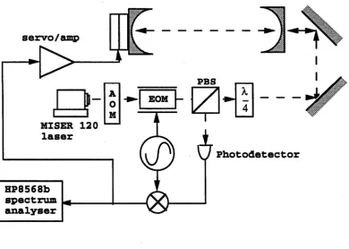
Figure 3.4A: Schematic of the experimental arrangement. The main components are the diode laser current supply; the diode laser; the Nd:YAG; two photo-detectors (PD1 & PD2) to be used in the control loop and as an out-of-loop monitor; an electronic PID servo system; and a drive circuit to feed the correction current into the current of the diode laser. Signals are injected into the loop at points A & C to measure the transfer functions of the loop.
Nd:YAG 350mW at
1064nm Diode Laser
1W at 810nm
Diode Laser
Current Supply
+1.8V
Beam Splitter
Spectrum
Analyser
Figure 3.4B: Simplification of Fig. (3.4A) using standard control theory topology. Note that G, in this case, represents the diode pump laser and the Nd:YAG crystal. H represents the PID electronics and the drive circuit for the diode laser. The shot noise on photodetectors PD1 and PD2 is uncorrelated and so is modelled as simple noise terms injected into the feedback system (PD1) and into the detected output light (PD2).
beam
splitter iNb(shot)
- x —
Ly-Sl PD2M
Na(shot)
w
v PD 1in loop
spectrum