Canny with Four Well Potential DRLSE Segmentation of Stem Cell Image

(1)

~ 120 ~ WWJMRD 2017; 3(7): 120-124

www.wwjmrd.com Impact Factor MJIF: 4.25 e-ISSN: 2454-6615

Nathiya.R Electronics and

Communication Engineering Pondicherry Engineering College Kalapet, Puducherry, India

Pratyusha M Electronics and

Communication Engineering Christ College of Engineering and Technology, Moolakulam Puducherry, India

Priyadarshini.C.N Electronics and

Sushmidha.R Electronics and

G.Sivaradje Electronics and

Communication Engineering, Pondicherry Engineering College, Kalapet, Puducherry, India

Correspondence: Nathiya.R Electronics and

Communication Engineering Pondicherry Engineering College Kalapet, Puducherry, India

Canny with Four Well Potential DRLSE Segmentation

of Stem Cell Image

Pratyusha M, Priyadarshini.C.N, Sushmidha.R, Nathiya.R, G.Sivaradje

Abstract

Stem cells are primal cells common to allmulticellular organisms that retain the ability to renew themselves through cell division. Self-renewal and Potency are the characteristic features of stem cells. An important and challenging task in the image analysis of stem cells is the image segmentation. Image segmentation is the partitioning of the digital image into various segments or sets of pixels. The proposed is a unification of canny edge detection technique and distance regularized level set method (DRLSE) with four well potential functions. Edge detection is a process which finds the boundary of objects within images by detecting discontinuities in brightness. The distance regularized level set method eliminates the need for re initialization which is present in most of the level set methods. A four well potential function is habituated to sustain the desired shape of level set function. First the edges are detected using canny operator followed by segmentation using the DRLSE algorithm.

Keywords: Stem Cells, Canny edge detector, Distance Regularized Level Set Evolution Algorithm (DRLSE)

Introduction

Image segmentation [3] is the division of an image into regions or categories, which correspond to different objects or parts of objects. Every pixel in an image is allotted to one of these categories. Pixels in the same category have similar greyscale and form a connected region whereas neighboring pixels which are in different categories have different values. Segmentation is the most critical step in image analysis. If segmentation is done well then all other stages in image analysis are made simpler. Segmentation algorithms are usually based on either discontinuity with sub regions, i.e. edges, or equality within a sub-region, though there are a few segmentation algorithms depends on both discontinuity and equality. A great variety of segmentation methods has been proposed in the past decades[13]. Level Set Method[9] is a one such method which was proposed for simpler image segmentation purpose. The level set method (LSM) is based on partial differential equations (PDE). Effortlessly, the LSM will converge at the boundary of the object where the differences are the highest.

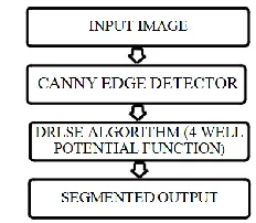
Methodology

Fig. 1: Segmentation Block Diagram

A. Input Images

(2)

pictures. The trailing and analysis of the morphological changes of cells are the difficult tasks in image processing. Stem cells[11] are terribly powerful cells found in both humans and non-human animals. The characteristic feature of stem cells is capability of dividing and revitalizing themselves for long periods. They will even produce specialized cell sorts. The time-lapsed video of neural stem cells is converted to frames. The frame rate is twenty nine frames/s, eight input pictures or frames are chosen, each at an associate degree interval of 8 hours. The Eight pictures chosen therefore on assess the expansion of the cells.

B. Canny Edge Detector

Canny edge detector was developed by John F.Canny in 1986. The boundaries are detected using multi stage algorithm.

Canny is termed as an optimal operator as a result of which it satisfies the subsequent conditions[2]:

 Accurately detecting as many edges as possible thereby resulting in low error rate.

 Accurate localization of edge point detected by the detector on the center of the edge.

 Any edge should be marked just once and also the false edges shouldn’t be chosen.

Among the edge detection ways developed up to now, like Sobel, Prewitt, Laplacian and Laplacian of Gaussian, Canny edge detection algorithm [18] is one of the most austerely well-defined ways that provides smart and dependable detection. There consist four steps in Canny Edge Detection. They are:

1. Noise Reduction: The Canny edge detector uses first derivative Gaussian filter as it is liable to noise present in pictures. The resultant image is slightly blurred compared to original image however there is absence of noise pixels in this picture.

2. Finding Intensity Gradient of Image: The horizontal, vertical and diagonal edges within the blurred image are identified by canny using four filters. The edge gradient and direction are calculated by

G = √Gx2 + Gy2 θ = arctan (Gy/Gx )

3. Non Maximal Suppression: Using the value of the image gradients, a pursuit is then administered to make a decision if the gradient magnitude takes up a local maximum in the gradient direction. A collection of edge points, within the form of a binary image, are obtained and as the name suggests if these points don’t have the local maxima value, they are suppressed.

4. Tracing Edges through the image and Hysteresis

Thresholding: Finally double threshold is applied to work out potential edges. All other edges that are weak and not connected to the strong edges are suppressed.

C. DRLSE Algorithm

The DRLSE [20] model provides an efficient segmentation without re-initialization. This methodology of active contours has become quite common for a range of applications, mainly image segmentation and motion tracking. The level set approaches move contours

completely as a particular level of a function. The central plan is to start out with initial boundary shapes presented in a type of closed curves, i.e. contours, and iteratively modify them by applying shrink/expansion operations according to the limitations of images. These operations, referred to as contour evolution, are done by the minimization of an energy function by the simulation of a geometric partial differential equation (PDE)[8]. The level set method (LSM) relies on partial differential equations (PDE), i.e. active analysis of the variations among neighboring pixels to seek out object boundaries. Effortlessly, the LSM can converge at the boundary of the item where the differences are the highest. LSM is used as a tool for numerical analysis of surfaces and shapes. During the evolution of contour because of the variation in velocity field of the image plane there occur irregularities of LSF [8], as a result the stability of the level set evolution is ruined and produce numerical errors. To eliminate this problem a numerical remedy called re-initialization [5] is used to revive the regularity of LSF and maintain stable level set evolution. The concept of initialization is to prevent the evolution instantly and re-modeling the disgraced LSF as a signed distance function.

Energy Formulation:

Let: φ: Ω→Ʀ be a level set function defined on domain Ω. An energy function ε(φ) is defined as:

ε(φ) = μ Ʀp(φ) +εext(φ)

Where μ>0 is a constant and Ʀp(φ) is the level set

regularization term, defined by

Ʀp (φ) = ∫p(∇∅ )dx

Where p signifies an energy density function p:[0,∞) →Ʀ is a potential function, it acts as the penalty term.

The energy εext(φ) is calculated such that it attains the zero

level set of the LSF is obtainable at desiderate position. The diminution of the energy ε(φ) can be reached by elucidating a level set evolution equation. A native alternative of the potential operator is p(s) = s2 for the regularization term Ʀp, which forces ∇φ to be zero. Such a

level set regularization term includes a stable leveling impact, however it tends to compact the LSF and create the zero level contours disappear. But, the aim of the level set regularization term isn’t solely to swish the LSF ϕ, but also to uphold the signed distance property ∇φ =1, at least in the range of the zero level set, so as to guarantee an careful valuation for curve evolution. This method can be done by applying potential p(s) function with a least possible point s=1, such that the level set regularization term (φ) Ʀp is minimized when ∇φ =1. Therefore, the

potential function should have a minimum point at s=1. The level set regularization term is referred to as a distance regularization term for its characteristic of actuality which is the signed distance property of the LSF. An exact definition of the potential for distance regularization is

p= (p1(s)(S-1)2 )/2

Which has s=1 as the unique minimum point. With this potential p = p1(s), the level set regularization term Ʀp can

(3)

P(φ)≜ 1/2 ∫(∇∅-1)2

The limit lies from [Ω →0), this typifies the eccentricity of φ from a signed distance function. The energy function is proposed to maintain the signed distance property in the entire process. The level set evolution for energy minimization has an unwanted side effect on the LSF in some cases. To evade this side effect, precede a new potential function p in the distance regularization term Ʀp.

The four well potential function is to preserve the signed distance property only in an area of the zero level set, although the LSF as a constant, with |∇φ |= 0, at locations far away from the zero level set. To exact quarter period for a particle in the Four-well potential as

√∫

√

Where w is the frequency, ag denotes the perturbation parameters, x0 is the origin point, u1 is the left well point,

u2 and u3 is the right well point and the limit ranges from 0

to x02 F is the elliptical integral function.

At middle well: Choosing the parameters as, a = u1,b = u2,

c = u3, d = x02 and then using the equation to find the exact

quarter period as

√

_√

( √

)

At left well: If the particle has negative energy, choose the parameters as a = u1,b = u2,c = u3, d = x02 and then using

the equation to find exact half period of particle with negative energy as

√

_√ ( √

)

At right well 1 and 2: If the particle has positive energy, choose the parameters as a=u1,b = u2,c = u3,d=x02 and then

find the exact half period as

√ _√ ( √

)

The problem with the existing DRLSE [15] model in the case of segmentation is that the curve will be induced and curves from the sketch in the region with untenable or without edges. So the proposed method is used to alter the distance regularization level set method (DRLSE) with four well potential functions.

D. Proposed Method Steps

 Convert the time lapse video into frames and save them as .jpg

 Select 8 images over an interval of 8 hours. These 8 frames are chosen so as to the indicate the mitotic division of stem cells

 If the image is in gray scale apply Canny Operator otherwise convert it to grayscale and apply canny

 Then find seed points for zero level contours

 DRLSE in which the regularity of the level set function is intrinsically maintained during the level set evolution. Then start level set evolution by DRLSE using four well potential functions

Experimental Results

This section shows the results of the proposed segmentation model. In the proposed model, two segmentation steps are applied. The initial step is the developing contour in the direction of the object borderline, when the evolving contour is distant from the object boundary, the process accelerates and when the evolving contour is near to the object boundary, the process slow down.

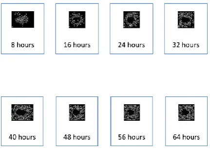
A. Input Images

The cell images are chosen at an interval of 8 hours each, which means that the first image is chosen at 0 hours, the second image at 8 hours, the third image at 16 hours and so on. These images are taken from a time lapse video of stem cells. As the hours progress the cells divide at a higher rate. Then these images are given as input to the canny operator.

Fig. 2: Input Images of Stem Cells

B. Canny Edge Detector Images

The images of the stem cells are given as input to the Canny Edge Detector [14]. The steps followed in Canny Edge Detector are as listed above. The Canny algorithm [7] is adaptable to various environments. Its parameters allow it to be couturier to recognition of edges of divergent features liable on the particular wants of a given implementation.

Fig. 3: Canny Operator Output Images

(4)

Define abbreviations and acronyms the first time they are used

C. Segmentation Output

Fig. 4: Segmented Output Images of Stem Cells

The proposed method of segmentation outputs are simulated for the time lapse images of the mesenchymal stem cell. By using the DRLSE [6], the level set evolution of the input image is done and the LSF for the input image are obtained.

The above figure 4 has the segmented images of stem cells, such that each of the following images has grown under similar circumstances with an evaluated time of 8 hours correspondingly. In the proposed model, two segmentation steps are applied. The initial step is the developing contour in the direction of the object borderline, when the evolving contour is distant from the object boundary, the process accelerates and when the evolving contour is near to the object boundary, the process slows down. The next step is to discern the segmentation results.

D. Performance Evaluation

The modified distance regularized level set segmentation method is evaluated by the boundary displacement error, PSNR values, Precision, and Recall. The Boundary Displacement Error (BDE) measures the average displacement error of one boundary pixels and the closest boundary pixels in the other segmentation. The precision and recall values describe the agreement between the focused on boundary edge elements of region boundaries of two segmentations. The four well potential function decreases the BDE, but when combined with the canny edge detector the BDE values are further more reduced and this avoids the over segmentation problems.

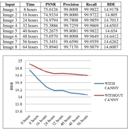
Table 1 Evaluation of DRLSE Four well Potential with Canny Edge Detector

Input Time PSNR Precision Recall BDE

Image 1 8 hours 75.0126 99.8008 99.9822 14.7556 Image 2 16 hours 74.9334 99.8000 99.9722 14.5047 Image 3 24 hours 74.9794 99.7808 99.9859 14.2850 Image 4 32 hours 75.3886 99.7259 99.9869 14.1753 Image 5 40 hours 75.2675 99.8081 99.9822 14.1799 Image 6 48 hours 75.0570 99.8008 99.9649 14.1120 Image 7 56 hours 75.3451 99.6590 99.9559 14.0958 Image 8 64 hours 75.8940 99.7170 99.9879 14.0648

BDE values signify the accuracy of the segmentation. The lesser the BDE values the higher is the accuracy. The

PSNR calculates the peak signal-to-noise ratio between two images, in decibels. This ratio is often used as a quality measurement between the original and a resultant image. The higher PSNR, the better the quality of the output image. To compute the PSNR, mean-squared error calculated is used. Precision is the proportion of boundary pixels in the automatic segmentation that correspond to boundary pixels in the ground truth. Precision and recall are attractive as measures of segmentation quality because they are sensitive to over and under-segmentation, over-segmentation leads to low precision scores, while under-segmentation leads to low recall scores.

Recall is defined as the proportion of boundary pixels in the ground truth that were successfully detected by the automatic segmentation.

Table 2: Evaluation of DRLSE Four well Potential

Input Time PSNR Precision Recall BDE

Image 1 8 hours 75.0126 99.8008 99.9822 14.9178 Image 2 16 hours 74.9334 99.8000 99.9722 14.805 Image 3 24 hours 74.9794 99.7808 99.9859 14.7013 Image 4 32 hours 75.3886 99.7259 99.9869 14.6503 Image 5 40 hours 75.2675 99.8081 99.9822 14.654 Image 6 48 hours 75.0570 99.8008 99.9649 14.6412 Image 7 56 hours 75.3451 99.6590 99.9559 14.6262 Image 8 64 hours 75.8940 99.7170 99.9879 14.6007

Fig. 5: Comparison of BDE values of Proposed Method and DRLSE with four well potential.

The above graph is the comparison of the BDE values of the proposed method (Canny edge detector with DRLSE four well potential functions) and the original DRLSE method using four well potential functions. From this it can be verified that since the proposed method has the lower BDE values, the image is segmented with utmost accuracy.

Conclusion

(5)

with over-segmentation problems observing with the DRLS model and has lower BDE values thereby producing accurate segmentation.

References

1. V. Torre and T. A. Poggio. “On edge detection”. IEEE Trans. Pattern Anal. Machine Intell., vol. PAMI-8, no.2, Mar. 1986, pp. 187-163.

2. J.Canny, “A Computational Approach to Edge Detection”. IEEE Transactions on Pattern Analysis and Machine Intelligence, 8(6),1986, pp.679-698. 3. Rajeshwar Dass, Priyanka, Swapna Devi “Image

Segmentation Techniques” IJECT ISSN : 2230-7109 | ISSN : 2230-9543 Vol. 3, Issue 1, March 2012 4. Punam Thakare “A Study of Image Segmentation and

Edge Detection Techniques”, International Journal on Computer Science and Engineering, Vol 3, No.2, 899- 904, (2011).

5. M. Sussman, P. Smereka, S. Osher, “A level set approach for computing solutions to incompressible two-phase flow”. Journal of Computation physics, 144(1), 1994 , pp.146-149.

6. C. Xu and J. Prince, “Snakes, shapes, and gradient vector flow, ”IEEE Trans. Image Process., vol. 7, no. 3, pp. 359–369, Mar. 1998.

7. S. Osher and R. Fedkiw, “Level Set Methods and Dynamic Implicit Surfaces” New York: Springer-Verlag, 2002.

8. C. Li, C. Xu, C. Gui, and M. D. Fox, “Level Set Evolution without Re-initialization: A New Variational Formulation,” in Proc. IEEE Conf. Comput. Vis. Pattern Recognit., 2005, vol. 1, pp. 430– 436.

9. F. Yang et al., “Cell Segmentation, Tracking, and Mitosis Detection Using Temporal Context,” Proceedings of MICCAI 2005.

10. T.A. Mohmoud; S.Marshal, “Edge –Detected Guided Morphological Filter for Image sharpening”, Hindawi Publishing corporation EURASIP Journal on image and video Processing volume 2008.

11. Dr. SachinAvasthi , Dr. R. N. Srivastava , Dr. Ajai Singh, and Dr. ManojSrivastava, “ Stem Cell: Past, Present and Future- A Review Article”, Internet Journal of Medical Update, Vol. 3, No. 1,pp 24-30; Jan-Jun 2008.

12. Jiafu Jiang , He Wei , Qi Qi ,” Medical Image

Segmentation Based on Biomimetic Pattern

Recognition”, World Congress on Software

Engineering,IEEE Computer Society. Vol:2,Pp.375-379,2009.

13. C. Li, C. Xu, C. Gui, and M. D. Fox,”Distance Regularized Level Set Evolution and Its Application to Image Segmentation”, IEEE Transactions Image Process, vol. 19, no. 12, pp. 3243–3253, Dec. 2010. 14. Saket Bhardwaj, Ajay Mittal “A Survey on Various

Edge Detector Techniques” Procedia Technology 4, 2012, 220 – 226.

15. Weifeng Wu, Yuan Wu and Qian Huang, “An Improved Distance Regularized Level Set Evolution without Re-initialization”, IEEE fifth International Conference on Advanced Computational Intelligence (ICACI )October 18-20, 2012.

16. Amir Rajaei, LalithaRangarajan and

ElhamDallalzadeh (2012) Medical ImageTexture Segmentation Using Range Filter. CS & IT 04: 273–

280.

17. Martin Maˇska, OndˇrejDanˇek, SarayGarasa, Ana Rouzaut, ArrateMu˜noz-Barrutia, and Carlos Ortiz-de-Sol´orzano, “Segmentation and Shape Tracking of Whole Fluorescent Cells Based on the Chan-Vese Model” IEEE Transactions On Medical Imaging,2013. 18. Indrajeet Kumar, Jyoti Rawat, Dr. H.S. Bhadauria “A Conventional Study Of Edge Detection Technique In Digital Image Processing” IJCSMC, Vol. 3, Issue. 4, April 2014, pg.328 – 334

19. Kusumanchi Avinash kumar, Satya Swathi Bylapudi (2014) “ An Adaptive Technique for Regularized Level Set Evolution to Image Segmentation” IOSR

Journal of Electronics and Communication

Engineering 9.