A comparative analysis of two Y-factor techniques
.
White Rose Research Online URL for this paper:
http://eprints.whiterose.ac.uk/723/
Article:
Collantes, J.M., Pollard, R.D. and Sayed, M. (2002) Effects of DUT mismatch on the noise
figure characterization: A comparative analysis of two Y-factor techniques. IEEE
Transactions on Instrumentation and Measurement, 51 (6). pp. 1150-1156. ISSN
0018-9456
https://doi.org/10.1109/TIM.2002.808015
[email protected] https://eprints.whiterose.ac.uk/
Reuse See Attached
Takedown
If you consider content in White Rose Research Online to be in breach of UK law, please notify us by
Effects of DUT Mismatch on the Noise Figure
Characterization: A Comparative Analysis of Two
Y-Factor Techniques
Juan-Mari Collantes, Member, IEEE, Roger D. Pollard, Fellow, IEEE, and Mohamed Sayed, Member, IEEE
Abstract—Device mismatch seriously degrades accuracy in
noise figure characterization. The suitability of corrections to the gain definitions for a more precise noise figure evaluation for mismatched devices is investigated and compared to classical techniques. The effects of device mismatch on the noise figure of the noise-meter receiver and its impact on the final accuracy are analyzed.
Index Terms—Microwave characterization, noise figure, noise
measurements, noise temperature, vector corrections, Y-factor technique.
I. INTRODUCTION
W
ITH the increasing need for high-performance compo-nents for use in mobile communications, the accurate measurement of the noise figure becomes an essential task. A significant number of procedures, addressing the issue of accurate noise figure calculation of circuits and devices, have been proposed in the recent literature [1]–[4]. The most common method for measuring the noise figure is the classical Y-factor technique, in which only noise power measurements are required [5]. Classical Y-factor is an accurate procedure for noise figure characterization provided that all the components involved in the measurement [noise source, device under test (DUT) and noise receiver] are well matched. However, because of the use of scalar noise power measurements alone, it cannot correct for the errors related to any mismatch present in the measurement path. In most cases, the noise source and the receiver are relatively well matched, and their effect can be neglected. Increasingly, there are requirements for mismatched devices to be measured, especially discrete active components (FETs, BJTs, etc.) presenting highly mismatched characteris-tics. Therefore, DUT mismatch becomes a critical issue in the noise figure characterization.Recently, a specific technique has been proposed in order to deal with mismatch effects in the noise figure evaluation [3]. This technique combines the classical Y-factor method
Manuscript received September 27, 2000; revised September 30, 2002. This work was supported in part by the University of the Basque Country.
J.-M. Collantes is with the Electricity and Electronics Department, University of the Basque Country, Bilbao, Spain.
R. D. Pollard is with the School of Electronic and Electrical Engineering, The University of Leeds, Leeds, U.K.
M. Sayed is with Agilent Technologies, Santa Rosa, CA 95403 USA. Digital Object Identifier 10.1109/TIM.2002.808015
with scattering parameter measurements. From these additional vector measurements, some corrections are performed on the classical procedure, the most important being those related to an accurate gain definition. The DUT gain is required in order to de-embed the noise figure of the DUT from the noise figure of the complete measurement system. The classical Y-factor technique makes use of the DUT insertion gain, since it is obtained through scalar measurements alone. Instead, the use of the DUT available gain, which can be computed from the measured -parameters, is proposed in [3]. In the following, we will refer to the use of the available gain for the noise figure calculation instead of insertion gain as the corrected Y-factor
technique.
In this work, the suitability of using the available gain and its actual effect on the measurement accuracy are analyzed and compared with the classical Y-factor technique. All the conse-quences derived from measurement of a mismatched DUT are investigated in detail. In particular, special attention is paid to the impact of DUT mismatch on the noise figure of the noise-meter receiver since this is required for the computation of the DUT noise figure. As the noise figure of the noise-meter re-ceiver can be a strong function of the source impedance con-nected to its input, we can expect significant variations in the receiver noise figure versus DUT output match. Here, the effects of neglecting the receiver noise figure dependence on source impedance are rigorously examined. Although there are other sources of error in any noise figure measurement (ENR un-certainty, instrument unun-certainty, presence of spurious signals, etc.), these are beyond the scope of this work.
It is first necessary to provide some basic definitions con-cerning the noise figure and related quantities and the funda-mentals of the Y-factor method. Its implementation through the classical and the modified techniques is described, and an un-certainty analysis, comparing both techniques, is performed as a function of DUT gain and match. Finally, some experimental data is presented which confirms the theoretical analysis.
II. RELEVANTNOISEFIGUREBASICS A. Noise Figure Definition
The noise figure is defined as the ratio of the signal-to-noise ratio (SNR) at the input of a two-port network to the SNR ob-served at the output when the input noise corresponds to the
available thermal noise power of a resistive termination at a ref-erence temperature (a value of K was first sug-gested by Friis [6])
(1)
where
and signal power levels available at the input and the output of the two-port network;
and available noise power at the input and the output of the two-port network.
can be expressed as
(2) where
noise power added by the two-port network; its available gain, which is described by
(3) Here, are the parameters of the two-port network, the reflection coefficient of the source connected at the input of the two-port network, and the output reflection coefficient of the two-port network
(4) Equation (1) can be rewritten as
(5) which is the definition of the noise figure at the standard refer-ence temperature, K, given by IEEE Standard [7].
B. Noise Parameters
A significant characteristic of the noise figure is that it is a function of the source impedance from which the device is fed. This dependence makes the noise figure an incomplete noise description of the device. The full characterization of the noise figure for all possible source terminations requires a set of four independent parameters. There are a variety of parameter sets that can be used to represent this dependence. One of the most commonly used sets is given by [8]
(6) where is the source reflection coefficient, is the reference impedance, and , , , and are the four classical noise parameters.
It is important to notice that, as tends to the edge of the Smith chart, the noise figure of any two-port network tends to infinity at a rate that is mainly determined by . In the limit, for a totally reflective source the noise figure is infinite, which is a straightforward result from (6).
C. Measuring Noise Figure: The Y-factor Method
The most widely used procedure to measure the noise figure is the Y-factor method [5]. It requires measurement of the noise power at the output of the DUT for two different (hot and cold) temperatures of the noise source. The ratio of these two power noise levels, and , is called the Y-factor, which gives the name to the technique
(7) From (5) the noise figure can be expressed as a function of the hot and cold noise source temperatures , the Y-factor and the reference temperature K
(8) Equation (8) assumes that the reflection coefficient of the noise source remains constant from hot to cold states. In practice, some amount of variation in should be expected. Since the noise figure is a function of the source impedance (6), variations will lead to some amount of error when (8) is used for the noise figure calculation. However, changes in from hot to cold states are small for typical commercial noise sources operated below 18 GHz and will be neglected in the following analyzes.
D. Second-Stage Correction
Equation (8) represents an ideal approach to the noise figure characterization of a generic DUT. However, in any real char-acterization setup, the measurement system also adds its own noise to the total output measured noise power. A typical con-figuration for noise figure measurement is depicted in Fig. 1(a) where the DUT is cascaded with a real receiver that also con-tributes to the total output noise.
The global noise figure of the cascaded system com-prising a DUT followed by a real receiver can be calculated from the measured output noise powers and by using (8). Then, the noise figure of the DUT can be de-embedded by making use of the Friis formula for the cascade of two stages:
(9) where
reflection coefficient of the noise source; output reflection coefficient of the DUT (4); DUT available gain (3);
noise figure of the receiver.
It is important to notice that, from (9), the noise figure of the DUT depends on three terms:
• the measured global noise figure of the system made up of the cascade of DUT and receiver, ;
• the noise figure of the receiver when the DUT is connected
to its input, , i.e., when the source impedance connected to its input is equal to ;
• the available gain of the DUT, .
(a)
[image:4.612.43.281.63.271.2] [image:4.612.303.557.73.294.2](b)
Fig. 1. Block diagram for noise figure measurements. (a) Measurement setup. The source impedance at the input of the receiver is0 . (b) Calibration setup. The source impedance at the input of the receiver is0 .
to make the second term of (9) negligible, then becomes equal to . Otherwise, knowledge of all three terms is re-quired to accurately determine the noise figure of the DUT.
III. TWOY-FACTORTECHNIQUES
Although (9) defines the “true” second-stage correction, it is almost invariably simplified in practice. Two noise-figure tech-niques that approximate (9) in two different ways are discussed next: the classical Y-factor technique and the corrected Y-factor technique. Both techniques are only approximations of the true second-stage correction. In both cases the quality of the approx-imation is a function of the DUT match and gain, and this is an-alyzed in the present work.
A. Classical Y-Factor Technique
This technique is the most extended way for measuring the noise figure, and it is based on noise power measurements ex-clusively [5]. The measurement procedure is divided into two steps. Step 1 is a calibration stage in which the noise source is directly connected to the receiver in order to measure the re-ceiver noise figure. The calibration configuration is depicted in Fig. 1(b). The result is the value of the receiver noise figure for a source impedance . Since the noise source has an at-tenuator pad at its output, it presents a reasonably good match and is usually close to zero. Thus, in general, the result from the calibration step corresponds to the receiver noise figure for well-matched source impedance conditions, . In step 2, the global noise figure of the cascaded system DUT and receiver is measured as shown in Fig. 1(a).
The available gain of the DUT, that is also required in (9), cannot be determined from scalar power measurements alone. Therefore, this technique calculates the insertion gain in-stead. Insertion gain is usually measured as the ratio of the power delivered when the DUT is connected between the noise
source and the receiver to the delivered power when the noise source alone is directly connected to the receiver
(10) The noise power measurements performed in steps 1 and 2 pro-vide the data required to compute the insertion gain from (10). The insertion gain can also be expressed as
(11) where:
parameter (input reflection coefficient) of the receiver;
and DUT -parameters;
reflection coefficient of the noise source; output reflection coefficient of the DUT (4). Equation (11) is only equal to the available gain when the DUT is perfectly matched.
The classical Y-factor technique then computes the DUT noise figure from:
(12) There are two potentially significant differences between the rigorous noise figure calculation from the true second-stage cor-rection (9) and (12) used by the classical Y-factor technique:
• is approximated by ; • is approximated by .
In the case of a highly mismatched DUT, the output reflec-tion coefficient (4) will differ greatly from , and signifi-cant discrepancies between and have to be expected. Only when the DUT is well-matched (mainly output match) does the receiver noise figure calculated during the cal-ibration step [Fig. 1(b)] coincide with the receiver noise figure during the measurement step [Fig. 1(a)] . Similarly, when the receiver and the noise source are per-fectly matched, is equal to . If, in addition, the DUT presents a good match, also converges to . Other-wise, can be significantly different from , especially for DUTs presenting a high output mismatch.
B. Corrected Y-Factor
Some corrections for improving noise figure accuracy have been recently proposed in [3]. The most significant of them takes into account the DUT mismatch by using the available gain in the second-stage correction, as required by (9). The available gain is calculated from the measured scattering param-eters of the DUT. and are obtained through the same calibration and measurement steps as the classical technique [Fig. 1(a) and (b)]. As a result, the DUT noise figure is determined from:
• is approximated by .
The same discussion concerning the discrepancies between and for mismatched DUTs that affected the classical Y-factor technique still holds for the corrected tech-nique.
IV. UNCERTAINTYANALYSIS
Equations (12) and (13) represent two different approxima-tions of the true second-stage correction given by (9). Both approaches substitute the term in (9) by the term measured during the calibration step. In addition, the classical technique also substitutes the available gain by the measured insertion gain , while the corrected technique makes use of the correct available gain obtained from measured -parameters. In this section, the uncertainty in the noise figure calculation from the two approximations is analyzed.
Let and be the noise figures calculated from the classical (12) and the corrected technique (13), respec-tively, and let be the actual noise figure computed from the true second-stage correction of (9). We can define the errors (in dB) in the noise figure calculation derived from both techniques as
(14) (15) From (9), (12), and (13), and can be expressed as
(16)
(17) and can be computed analytically by knowing the DUT characteristics (noise figure and -pa-rameters), the receiver characteristics ( and the four noise parameters), and the noise source reflection coefficient ( . It is important to recall that the errors given by eqs. (16) and (17) are exclusively related with the way the “true” second-stage cor-rection is approximated by eqs. (12) and (13). Other uncertainty sources present in any type of noise figure measurement (ENR uncertainty, instrument uncertainty, etc.) are not included.
While the receiver and the noise source characteristics are fixed and unchanged for a given measurement system, DUTs of very different gain, match and noise figure may be measured. The example analysis evaluates and as functions of the DUT gain and match using the parameters listed in Table I.
Some considerations concerning this analysis have to be high-lighted.
• Equations (16) and (17) are not explicit functions of fre-quency. Therefore, frequency is not directly involved in the analysis. All the terms used to compute
TABLE I
VALUES OFPARAMETERSUSED IN THEANALYSIS
Fig. 2. Magnitude of the error versus DUT output return loss. Three values ofS are considered. Characteristics of DUT, noise source and noise-meter receiver are listed in Table I. Solid line: classical. Dashed line: corrected.
and (receiver noise parameters, DUT -pa-rameters, DUT noise figure, etc.) are given at a single fre-quency point.
• The generic noise source and receiver, with common pa-rameter values, are used in the analysis. is a value typical of commercial noise sources used for applications below 18 GHz. The changes in from hot to cold states are neglected.
• A DUT with noise figure dB is used. The DUT output return losses will range from 30 dB to 1 dB. Input match is constant since the impact on the final error is less significant provided that the noise source is well matched. Three values of are considered: 5, 10 and 20 dB.
V. RESULTS ANDDISCUSSION
Fig. 2 shows the absolute value of the error in the noise figure obtained from the two techniques, versus the DUT output return losses, and for the different values of DUT . Several general observations may be made.
Fig. 3. Receiver noise figureF as a function of DUT output return loss.
(13). High values of make this second term negligible, and all three equations yield similar results.
• Errors are reduced in both techniques as the output return losses of the DUT decrease. This is due to the fact that, as the DUT output match improves, converges to , and to (provided that the noise source and the receiver are reasonably well-matched, which is commonly the case).
• For low gain and high output mismatch both techniques provide a considerable amount of error.
The remarkable conclusion of this analysis is that, the cor-rected technique only presents a benefit for low values of the DUT output return loss, while the classical technique still pro-vides a lower amount of error for high output return losses. This result may seem paradoxical given that the corrected technique makes use of the available gain in order to better take into account mismatch effects, while the classical technique substi-tutes by the insertion gain instead.
However, this phenomenon has a subtle explanation. The re-ceiver noise figure and the DUT available gain ap-pearing in (9) are strong functions of the device output match through [see (3) and (6)]:
— , in the numerator of (9), is inversely pro-portional to the term .
— , in the denominator of (9), is also inversely proportional to the term .
In both cases, the term becomes dominant as the DUT output match worsens , which makes and tend to infinity. This is graphically shown in Figs. 3 and 4, where and are plotted as functions of the DUT output return losses. The two curves are calculated considering the same receiver and noise source characteristics (Table I) and a DUT of 5 dB. Superimposed in Fig. 3 is the receiver noise figure obtained from the calibration step , which is obviously independent of . Also, the insertion gain for the same DUT is plotted in Fig. 4, showing only a slight dependence on . Since
[image:6.612.310.551.61.239.2]and have the same form, they tend to compensate each other in (9). The corrected Y-factor combines —a
Fig. 4. Available gainG and insertion gain G as functions of DUT output return loss.
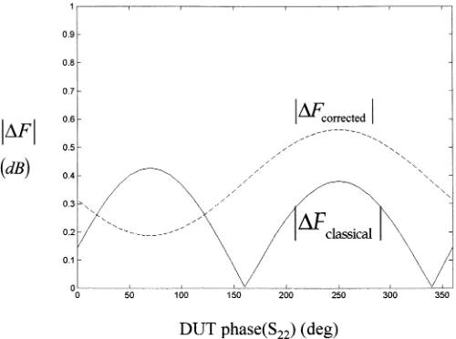
Fig. 5. Noise figure errorsj1F j and j1F j as functions of the DUT phase (S ) for DUT characteristics: S = 5 dB, S = 08 dB, andF = 2 dB. (Other parameters as in Table I).
strong function of —with —independent of —resulting in large errors as the mismatch degrades. Conversely, the classical Y-factor combines with that is only a mild function of , which can result in a smaller total error.
This explanation is not necessarily a general result. Which one of the two techniques provides the more accurate results de-pends strongly on the receiver and DUT characteristics (receiver noise parameters, receiver match, DUT -parameters, etc.). As a first example, Fig. 5 shows and as a function of the phase of the DUT . Other characteristics of the DUT are dB, dB and dB with the remainder of the parameters involved in the analysis from Table I. Notice that errors strongly depend on phase conditions. Moreover, for some phases the smallest error is provided by the classical Y-factor technique, while for other phases the smallest error is associated with the corrected Y-factor.
[image:6.612.303.553.280.466.2]Fig. 6. Noise figure errorsj1F j and j1F j as functions of the receiver noise resistanceR for DUT characteristics: S = 5 dB, S = 05 dB, phase (S ) = 25 , and F = 2 dB. (Other parameters as in Table I).
]. The rest of the elements in the analysis are those from Table I. We can observe how, for this particular example, the classical Y-factor presents a smaller error for high , whereas the corrected Y-factor is more accurate for low .
Similar curves to Figs. 5 and 6 can be obtained by sweeping the other parameters involved in the analysis , always resulting in the same conclusion: no general statement, valid for any arbitrary DUT and receiver characteristics, can be made about the suitability of using one of the two techniques, either or both of which may give highly erroneous results.
A precise application of the Y-factor method, suitable for low-gain, highly mismatched devices, would also need the eval-uation of the term in the second-stage correction (9). To do so, the four noise parameters of the receiver must be known or determined at a previous stage, so that
can be computed from (6).
VI. EXPERIMENTALDATA
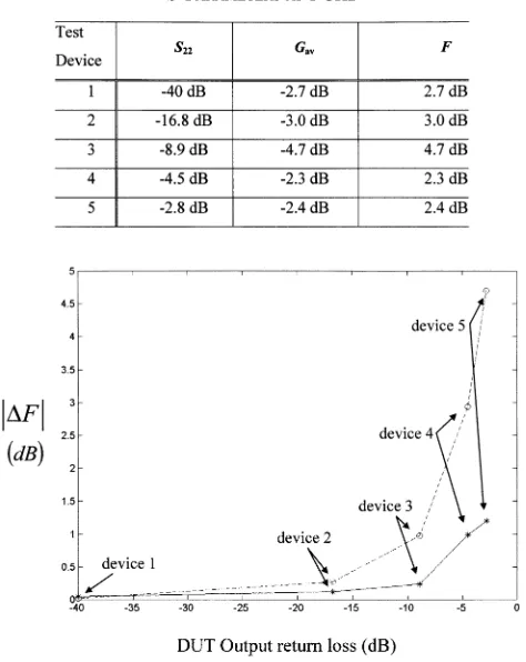
The results presented in the previous analysis have been ver-ified with experimental data. The two Y-factor techniques have been applied to the noise figure measurement of five passive de-vices, each one having a different output match. These devices are built up combining a pad with different output mismatch blocks. Note that passive devices are selected for this experi-ment since their “true” noise figure can be calculated analyti-cally from the -parameters (for passive devices the noise figure is the inverse of the available gain). As a first step, the -pa-rameters of each device are measured at 1 GHz with a vector network analyzer. The resulting available gain and noise figure, computed from the -parameters, are listed in Table II.
Then, the noise figures of the five devices were measured at 1 GHz through both the classical and corrected Y-factor tech-niques using a specific in-house noise-meter receiver with a noise figure of 4.1 dB and the HP 346B noise source. Note that the available gain calculated from the -parameters (Table II) was used in the computation of the corrected Y-factor.
The errors associated with each technique ( and ) can be easily obtained since the “true” noise
TABLE II
DATA FOREXPERIMENTALDEVICESCOMPUTEDFROM THEMEASURED
[image:7.612.309.546.89.387.2]S-PARAMETERS AT1 GHz
Fig. 7. Measuredj1F j and j1F j for five devices with different output return loss. Solid line: classical. Dashed line: corrected.
figures of the five passive devices have already been determined from the measured -parameters. Fig. 7 shows
and as a function of the device output return loss. As expected, both errors dramatically increase as the device output match worsens. It is important to note that, since the gain of these passive devices is lower than unity, the mismatch errors are significantly higher. Nevertheless, for this series of experiments, results were always better with the classical Y-factor technique, confirming that there is no general benefit gained by using the available gain to correct the results when the DUT output return loss is high. In addition, the experiments yielded similar outcomes regardless of any additional cable length (phase shift) added to the devices.
VII. CONCLUSION
ensure a more accurate result for high values of DUT output return losses. Errors from both techniques are strong functions of the receiver and DUT characteristics.
ACKNOWLEDGMENT
The authors would like to thank B. Shoulders of Agilent Tech-nologies for helpful discussions.
REFERENCES
[1] C. E. Collins, R. D. Pollard, R. E. Miles, and R. G. Dildine, “On the measurement of SSB noise figure using sideband cancellation,” IEEE Trans. Instrum. Meas., vol. 45, pp. 721–727, June 1996.
[2] R. Drury, R. D. Pollard, and C. M. Snowden, “W-band noise figure mea-surement designed for on-wafer characterization,” in IEEE MTT-S Int. Microwave Symp. Dig., 1996, pp. 1273–1276.
[3] D. Vondran, “Noise figure measurement: Corrections related to match and gain,” Microwave J., pp. 22–38, Mar. 1999.
[4] S. C. Bundy, “Noise figure, antenna temperature and sensitivity level for wireless communications receivers,” Microwave Journal, pp. 108–116, Mar. 1998.
[5] “Fundamentals of RF and microwave noise figure measurements,” Hewlett-Packard Application Note 57-1, Palo Alto, CA, July 1983. [6] H. T. Friis, “Noise figures of radio receivers,” Proc. IRE, pp. 419–422,
July 1944.
[7] “Description of the noise performance of amplifiers and receiving sys-tems,” Proc. IEEE, pp. 436–442, Mar. 1963. Sponsored by IRE subcom-mittee 7.9 on Noise.
[8] G. Gonzalez, Microwave Transistor Amplifiers. Englewood Cliffs, NJ: Prentice-Hall, 1984.
Juan-Mari Collantes (M’96) was born in Bilbao, Spain, in 1966. He received
the degree in electronic physics from the University of the Basque Country, Spain, in June 1990 and the Ph.D. degree in electronics from the University of Limoges, Limoges, France, in March 1996. In December 1997, he received the Ph.D. degree in electronics from the University of Cantabria, Cantabria, Spain. Since February 1996, he has been an Associate Professor in the Electricity and Electronics Department, University of the Basque Country. From July to December 1996, he was a Visiting Researcher at Hewlett-Packard, Santa Rosa, CA. His areas of interest include nonlinear analysis of microwave circuits, non-linear modeling of microwave devices, and noise characterization at microwave frequencies.
Roger D. Pollard (M’77–SM’91–F’97) was born in
London, U.K., in 1946. He received the B.Sc. and Ph.D. degrees in electrical and electronic engineering from the University of Leeds, Leeds, U.K.
He holds the Agilent Technologies Chair in High Frequency Measurements and is Head of the School of Electronic and Electrical Engineering, University of Leeds, where he has been a faculty member since 1974. He is an active member of the Institute of Mi-crowaves and Photonics (one of the constituent parts of the School) which has over 40 active researchers, a strong graduate program, and has made contributions to microwave passive and active device research. The activity has significant industrial collaboration as well as a presence in continuing education. Professor Pollard’s personal re-search interests are in microwave network measurements, calibration and error correction, microwave and millimeter-wave circuits, terahertz technology, and large-signal and nonlinear characterization. He has been a consultant to Agilent Technologies (previously Hewlett-Packard Company), Santa Rosa, CA, since 1981. He has published over 100 technical articles and three patents.
Prof. Pollard is a Chartered Engineer and a Fellow of the Institution of Elec-trical Engineers (U.K.). He is an active IEEE volunteer (as an elected member of the Administrative Committee and 1998 President of the IEEE Microwave Theory and Techniques Society and as 2001/2002 Chair of the Products Com-mittee) and a Member of the IEEE Technical Activities Board and Vice-Chair of the Publications, Services and Products Board (PSPB). He was Chair (1998 to 2000) of the TAB/PAB Electronic Products Committee which was respon-sible for the development and introduction of IEEEXplore. He has served as Chair of the UKRI Section and on many volunteer committees, groups, and working parties. He is a member of the Editorial Board of IEEE TRANSACTIONS ONMICROWAVETHEORY ANDTECHNIQUESand has been on the Technical Pro-gram Committee for the IEEE Microwave Theory and Techniques International Microwave Symposium since 1986. He edits the IEEE Press book series on RF and microwave technology.
Mohamed Sayed (M’73) was born in Cairo, Egypt He received the B.S. and
M.S. degrees in electrical engineering from Cairo University, Cairo. He received the Ph.D. degree from Johns Hopkins University (JHU), Baltimore, MD.
He was with Hewlett-Packard for 27 years and with Agilent Technologies for three years. He is currently an Engineering Project Manager of microwave vector network analyzers. He taught graduate and undergraduate courses at Cairo University, JHU, Howard University, Washington, DC, and San Jose State University, San Jose, CA. He has author and coauthor of over 32 publi-cations in the field of device characterization, microwave and millimeter-wave measurement systems, and high power amplifier design.