A multiple sequential orthogonal least squares algorithm for feature ranking and subset selection

This is a repository copy of

A multiple sequential orthogonal least squares algorithm for

feature ranking and subset selection

.

White Rose Research Online URL for this paper:

http://eprints.whiterose.ac.uk/74508/

Monograph:

Billings, S.A. and Wei, H.L. (2005) A multiple sequential orthogonal least squares algorithm

for feature ranking and subset selection. Research Report. ACSE Research Report no.

908 . Automatic Control and Systems Engineering, University of Sheffield

[email protected] https://eprints.whiterose.ac.uk/ Reuse

Unless indicated otherwise, fulltext items are protected by copyright with all rights reserved. The copyright exception in section 29 of the Copyright, Designs and Patents Act 1988 allows the making of a single copy solely for the purpose of non-commercial research or private study within the limits of fair dealing. The publisher or other rights-holder may allow further reproduction and re-use of this version - refer to the White Rose Research Online record for this item. Where records identify the publisher as the copyright holder, users can verify any specific terms of use on the publisher’s website.

Takedown

If you consider content in White Rose Research Online to be in breach of UK law, please notify us by

A Multiple Sequential Orthogonal Least Squares Algorithm for

Feature Ranking and Subset Selection

S. A. Billings and H. L. Wei

Research Report No. 908

Department of Automatic Control and Systems Engineering

The University of Sheffield

Mappin Street, Sheffield,

S1 3JD, UK

A Multiple Sequential Orthogonal Least Squares Algorithm for

Feature Ranking and Subset Selection

Stephen A. Billings and Hua-Liang Wei

Department of Automatic Control and Systems Engineering, University of Sheffield Mappin Street, Sheffield, S1 3JD, UK

[email protected], [email protected]

Abstract: High-dimensional data analysis involving a large number of variables or features is commonly encountered in multiple regression and multivariate pattern recognition. It has been noted that in many cases not all the original variables are necessary for characterizing the overall features. More often only a subset of a small number of significant variables is required. The detection of significant variables from a library consisting of all the original variables is therefore a key and challenging step for dimensionality reduction. Principal component analysis is a useful tool for dimensionality reduction. Principal components, however, suffer from two main deficiencies: Principal components always involve all the original variables and are usually difficult to physically interpret. This study introduces a new multiple sequential orthogonal least squares algorithm for feature ranking and subset selection. The new method detects in a stepwise way the capability of each candidate feature to recover the first few principal components. At each step, only the significant variable with the strongest capability to represent the first few principal components is selected. Unlike principal components, which carry no clear physical meanings, features selected by the new method preserve the original measurement meanings.

Keywords: Dimensionality reduction, high-dimensional data analysis, subset selection, principal component analysis, orthogonal least squares.

1. Introduction

Multivariate data analysis such as multiple regression and high-dimensional pattern classification, often

involves a large number of variables or features. Quite often the sample features are unknown a priori and

measurements are obtained with respect to more variables than is strictly necessary for conveying the main

features. There is, therefore, the potential to greatly reduce the dimensionality without distorting the overall

features. As one commonly used dimensionality reduction approach, subset selection aims to find a small

number of significant variables or features from a library consisting of all the original variables. The remaining

insignificant variables are, in a sense, irrelative or redundant, and can be ignored. In fact, the inclusion of these

insignificant variables may often complicate data inspection without providing any extra information [Jolliffe

1972].

A large amount of work has been done on dimensionality reduction, see for example, [Oja 1983, Jain et al.

2000, Carreira-Perpinan 2001, Fodor 2002, Webb 2002]. Principal component analysis (PCA) and its variants

[Jolliffe 2002] belong to the class of the most commonly used methods for dimensionality reduction. Note,

however, that principal components (PCs) suffer from two main drawbacks: PCs are transformed variables that

always involve all the original variables, and PCs are usually difficult to physically interpret. In many cases there

may be some redundancy, linear correlation or linear dependency among the original variables. The redundant or

to save a great amount of time and cost spent on obtaining and measuring these insignificant variables in future

experiments. Bearing this fact in mind, efforts have been made to develop algorithms to select significant

variables or eliminate insignificant variables from the full set of original variables, to form an effective subset

that can be used to sufficiently recover the main information conveyed by the full data set [Jolliffe 1972, 1973,

Krzanowski 1987, Pudil et al. 1994, Kohavi and John 1997, Mao 2005]. In fact, in many cases it is desirable to

reduce not only the dimensionality in the transformed space, but also the number of variables that need to be

considered or measured in the future in the measurement space [McCabe 1984].

This study introduces a new method for ranking significant variables and selecting a subset from a library

consisting of all the original variables. In the new method, a general variable detection and subset selection

problem is initially converted into a multivariate regression problem by treating principal components as the

dependent variables (responses) and the original variables as the independent variables (predictors or explanatory

variables). A new multiple sequential orthogonal least squares (MSOLS) algorithm is derived to detect the

significant variables for multivariate regression. The main idea behind the new method is to detect, in a stepwise

way, the significance of each candidate variable to represent the first few PCs. At each step only the variable

with the strongest capability to present the first few PCs is selected and included in the subset.

The paper is organized as follows. In Section 2 the multiple sequential orthogonal least squares method is

proposed in detail. In Section 3, the variable detection problem from principal components is converted into a

subset selection problem for multiple regression, for which significant variables can easily be detected using the

MSOLS algorithm. In Section 4, three examples relating to both artificial and real data sets are provided to

illustrate the application of the new method for feature ranking and subset selection. The work is briefly

concluded in Section 5.

2. The MSOLS algorithm

This section presents an orthogonal least squares type algorithm for variable detection and subset selection

for a multiple linear regression. The models that are considered throughout the paper will be restricted to the

linear in the regression coefficients form. The learning algorithm is multiple-regression oriented and will be

implemented using a sequential orthogonal least squares method. This new learning scheme will thus be referred

to as the multiple sequential orthogonal least squares (MSOLS) algorithm.

2.1 The multiple regression model

Denote the multiple response variables by and the set of n predictor (or independent) variables by . Assume that the relationship between (i=1,2, …,m) and (j=1,2, …,n) can be approximated by the linear-in-the-parameters regression model

m

y y y1, 2,L

n

x x

x₁, ₂,L, yi xj

) ( ) ( )

(

1 , 0

, x k e k

k

y _i

n

j

j j i i

i = +

∑

+

=

β

β

(1)

where denotes the kth observation of the ith response variable and denotes the kth observation of the

jth predictor variable (i=1,2, …, m; j=1,2, …, n; k=1,2, …, N); is assumed to be an unobservable error representing the discrepancy in the approximation; , called the regression parameters or

) (k

y_i x_j(k)

) (k e_i

n i i

i,0,

β

,1, ,

β

,

coefficients, are unknown constants that need to be estimated from the data. The linear model (1) can be

expressed using a compact form

i i

i X e

y = + (2)

where , , and

with and for j=1,2,…, n.

T i i

i

i=[e(1),e(2),L,e(N)] e

T i i

i

i =[y(1),y(2),L,y (N)]

y _i =[

β

_i,0,

β

_i,1,L,

β

_i,_n]T

T ] 1 , , 1 , 1 [

0 = L

x x_j =[x_j(1),x_j(2),L,x_j(N)]T ]

, , ,

[x0 x1 xn

X= L

The m matrix equations given by (2) can be put together to form an mth block-structured matrix equation below

e X

y=~ + (3) where

⎟⎟

⎟

⎟

⎟

⎠

⎞

⎜⎜

⎜

⎜

⎜

⎝

⎛

=

m

y

y

y

y

M

2 1 , , ,

⎟⎟

⎟

⎟

⎟

⎠

⎞

⎜⎜

⎜

⎜

⎜

⎝

⎛

=

m

e

e

e

e

M

2 1

⎟⎟

⎟

⎟

⎟

⎠

⎞

⎜⎜

⎜

⎜

⎜

⎝

⎛

=

m

M

2 1 X I X X X

X = ⊗

⎟⎟ ⎟ ⎟ ⎟ ⎠ ⎞ ⎜⎜ ⎜ ⎜ ⎜ ⎝ ⎛ = _m O O O O O O ~ L M M M M L L

whereOis a matrix whose all entries are zeros, the notation denotes the mth order unit matrix, and the symbol ‘ ’ denotes the Kronecker product, which is defined for two matrix and

as m

I

) 1 ( + ×m n N s r j i

a

_×

=

(

,

)

A

⊗ j i

b

(

, u×v

=

)

B

⎥

⎥

⎥

⎥

⎥

⎦

⎤

⎢

⎢

⎢

⎢

⎢

⎣

⎡

=

⊗

B

B

B

B

B

B

B

B

B

B

A

s r r r s s

a

a

a

a

a

a

a

a

a

, 2 , 1 , , 2 2 , 2 1 , 2 , 1 2 , 1 1 , 1

L

M

M

M

M

L

L

2.2 Subset selection for the multiple regression model

In many cases, the full set of the original predictor variables may be redundant for

representing the response variables, , because of linear correlation and dependency. Furthermore,

it is not necessary that all the n predictor variables are of the same importance for representing the response variables. The objective of subset selection is to find a subset

n

x

x

x

₀

,

₁

,

L

,

m

y

y

y

₁

,

₂

,

L

,

} , , { } , , { 1

1 d i i_d

d

S = z L z = x L x

, where ,

} , , ,

{ 0 1 n

S= x x L x

⊆

k

i

k x

z = i_k∈{0,1,L,n} (k=1,2, …, d), so that (i=1,2,…,m) can be satisfactorily approximated using a linear combination of as below

i y

d z z1,L,

i d d i i

i= ,1z1+ + , z +e

y

θ

L

θ

(4)

or, in a compact matrix form

i i i=Z +e

y (5)

where the matrix is of full column rank, is a parameter vector, and is an

approximation error vector.

T d i i

i =[

θ

,1,L,

θ

, ]

] , , [z1 zd

To select a subset for the multiple regression model, the significance of each variable needs to be detected

initially by inspecting the capability of each predictor variable to represent all the response variables. A subset

can then be determined by selecting the significant predictor variables or eliminating the insignificant predictor

variables. In the following, a new multiple sequential orthogonal least squares (MSOLS) method is proposed for

significant variable detection and subset selection.

2.3 The MSOLS algorithm for subset selection

The MSOLS algorithm starts from the mth order block-structured matrix equation (3). Let be the column vectors of the matrix X~

) 1 ( 2

1, ,L, mn+ . Define

) )( ( ) ( ] [ ERR 2 ) 1 ( j T j T j T j y y y

= , j=1,2,…, m(n+1), (6)

]}

[

ERR

{

max

arg

(1) ) 1 ( 1 1

j

n m j≤ + ≤

=

l

(7)

) 1 , mod( 1 0

1 = l n+

l (8)

n ≤ ≤ ₁ 0 l ) ,

mod(⋅⋅ ’ is defined as the modulus after division and thus

where the function ‘ . The meaning of

will be explained later. The first significant variable can then be selected as , and the

associated orthogonal variable can be chosen as ]

[

ERR(1) j 0

1 1 x_l

z =

1

1 l

q = .

Assume that a subset , consisting of (r-1) significant variables, , has been determined at step (r-1), and the (r-1) selected variables have been transformed into a new group of orthogonalized variables via some orthogonal transformation. To select the rth significant variable , let

for j=1,2,…,m(n+1) and . Orthogonalize

with as below

1 1, ,zr−

z L 1 − r S 1 2

1

,

q

,

,

q

r−

q

L

z_r

} 1 , , 2 , 1 for of multiple is :

{ 0 = −

=

∉ k r

j _r l l l_k L

j r j, =

1 2

1

,

q

,

,

q

r−

q

L

r j,

∑

− = − = 1 1 , , , r k k k T k k T k j r j r j q q q q

q (9)

Following [Korenberg et al. 1988, Billings et al. 1989, Chen et al. 1989], the error reduction ratio, ERR[j;r], produced by adding the jth data vector _j,r = _jinto Sr−1for representing the overall responseyis defined as

) )( ( ) ( ] [ ERR , , 2 , ) ( r j T r j T r j T r j q q y y q y

= (10)

Let ]} [ ERR { max arg (r) ) 1 (

1 j mn j

r = _{≤ ≤ +}

l (11)

) 1 , mod(

0 _{= +}

n

r

r l

l (12)

0

r

r x_l z =

The rth significant variable can then be chosen as , and the associated orthogonal variable can be chosen

as . Subsequent significant variables can be detected in the same way step by step. At each step, the

‘best’ variable that accounts for the variation of the overall response ywith the highest percentage is selected.

r r qlr,

The above variable detection procedure involves sequential orthogonal transformations. For example, at step

r, where a subset of r significant variables, , has been obtained. These r variables can be used to approximate the overall response with a linear form

r z z z₁, ₂,L,

r S y ) ( ) ( )

(r r _er P

y= + (13)

where [ , , , ] , (r)is the regression parameter vector, e(r)is the approximation error vector. 2 1 ) ( r r l l l L P =

From the above variable selection procedure, the full rank matrixP(r)can be orthogonally decomposed as

) ( ) ( )

(r r r

R Q

P = (14)

) (r R

where is a r×r unit upper triangular matrix and Q(r) is an r×r matrix with orthogonal columns . Substituting (14) into (13), yields

r

q

q

q

₁

,

₂

,

L

,

) ( ) ( ) ( ) ( ) ( ) ( 1 ) ( ) ( ] ][ ) (

[Pr Rr Rr r er Qrg r er

y= − + = + (15)

where is an auxiliary parameter vector. Using the orthogonal property of

, can be directly calculated from y and as for k=1,2, …,r. The unknown parameter vector can then be easily calculated from and

) ( ) ( ) ( ) ( 1 ) ( ] , ,

[ r _rr T r r

r _{g g R}

g = L =

) /( ) ( ) ( k T k k T r k

g = y q q q

) (r k g ) (r

Q Q(r)

) (r

g R(r)

) (r

by substitution using the special

structure ofR(r).

The total sum of squares of the overall response yfrom the origin can then be expressed as

) ( ) ( 1 2 ) ( ) ( )

( r T r

r k k T k r k T

g q q e e

y

y =

∑

+

= (16)

∑

= r k k T k r k g 1 2 ) ( )

( q q

Note that the total sum of squares yTy consists of two parts, the desired output , which can

be explained by the selected variables, and the part , which represents the residual sum of squares.

Thus, is the increment to the desired total sum of squares of the output brought by . The kth error reduction ratio (ERR) introduced by (or equivalently by ), is defined as [Korenberg et al. 1988,

Billings et al. 1989, Chen et al. 1989]

) ( ) (

) (er Ter

k T k r k

g( ))2q q

( q_k

k

q zk

) )( ( ) ( ] [ ERR 2 ) ( k T k T k T r _k q q y y q y

= , k=1,2, …, r, (17)

This ratio provides a simple but an effective index to indicate the significance of adding the kth variable into the model. The orthogonalization procedure for variable selection is usually implemented in a stepwise way, one

variable at a time. The sum of error reduction ratio (SERR) [Wei et al. 2004] due to

q

₁

,

q

₂

,

L

,

q

_ris defined as

∑

= = r k k r 1 (r) ] [ ERR ] [

continued and new significant variables need to be added to the subset, until the specified conditions are met.

The pseudo-code of the MSOLS algorithm developed on the basis of the forward Gram-Schmidt transformation

is given in Appendix A.

3. Detecting significant variables from PCs using MSOLS

Feature selection and feature extraction are two commonly encountered problems in statistical pattern

recognition. Unlike regression analysis, where the objective is to achieve an approximation of the relationship

between the response variables and the predictor variables and which can be solved using some supervised

learning schemes, a typical dimensionality reduction problem, for instance feature extraction and feature

selection in statistical pattern recognition, often involves a group of input data with a target to find significant

patterns or features but without a clearly defined external supervisor (the desired response). Thus, in many cases

the tasks of dimensionality reduction (subset selection) are fulfilled using some unsupervised learning algorithms

[Haykin 1999, Webb 2002, Jain et al. 2000].

As will be seen, the feature detection and subset selection problem for a general non-regression

high-dimensional data analysis can be directly converted into a multiple regression problem by treating the PCs as the

response variables and the original measurement variables as the predictors; the MOLS algorithms can then be

applied to detect significant variables and hence to select a subset.

3.1 PCA

Principal component analysis is a matrix based subspace decomposition method [Oja 1982, Jolliffe 2002],

where a covariance (or correlation) matrix is initially constructed from collected data, and associated eigenvalues

and eigenvectors (called direction vectors) of the covariance (or correlation) matrix are then calculated. Input

data vectors in the original measurement space can be orthogonally projected onto the subspace (the new feature

space) spanned by a few eigenvectors with maximum eigenvalues. The resulting projections are referred to as

principal components (PCs), the significance of PCs is evaluated by the corresponding eigenvalues. The basic

idea of PCA can briefly be summarized below.

Step 1. Data collection.

Assume that a total of N observations (patterns) are available and let

be the kth feature vector in the measurement space. The data matrix can then be represented as . Note that the collected data are often centralized or standardized.

T n k

x k x k x

k) [ ( ), ( ), , ( )]

( = _{1 2} L

x

T

N)] ( , ), 2 ( ), 1 (

[x x x

X= L

Step 2. Form the covariance (or correlation) matrix =(1/(N−1))XTX≈(1/N)XTX.

Step 3. Calculate the eigenvalues and eigenvectors of the matrix .

Step 4. Sort the eigenvalues and the eigenvectors. Rearrange the eigenvalues in decreasing order such that

n

λ

λ

λ

1≥ 2≥L≥ . Rearrange the eigenvectors accordingly and denote the rearranged eigenvectors by

n

, , , 2

1 L .

Principal component analysis aims to find a well-defined transform that maps the feature vectors in the n -dimensional measurement space to a new m-dimensional feature space without losing much information, where in general . Dimensionality can often be greatly reduced by introducing an orthogonal transform

involving only the first m eigenvectors , such that

) (k

x

n

m

<<

m

,

,

,

2

∑

=

= n

j

j j i x

1 ,

α

x

y_i= T_i (19)

where , and is referred to as the ith

principal component (PC) (i=1,2, …, m). PCA is perhaps the most commonly used transform for feature extraction. Note that each new variable in the new feature space is a linear combination of all the original

variables, this often makes it difficult to physically interpret the principal components in the new space.

T n

x x

x, , , ] [ 1 2 L =

x y_i =[y_i(1),y_i(2),L,y_i(N)]T

T n i i

i

i =[

α

,1,

α

,2,L,

α

, ]

3.2 Detecting significant variables of PCs

It has been noted that although the dimensionality may be greatly reduced, the number of variables need to

be measured in the original measurement space is kept the same. In cases where there exists some linear

dependency and linear correlation among the original variables, the inclusion of redundant variables in PCs is

not necessary. Subset selection is thus desired.

Let be the collected data matrix, where for j=1,2, …, n.

The vectors may be linearly dependent or correlated in the n-dimensional measurement space. The objective of subset selection is to find a subset

T j j

j

j =[x (1),x (2),L,x (N)] x

] , , ,

[x1 x2 xn

X= L

n x x x1, 2,L,

} , , , {

2 1 i id

i d

S = x x L x , which constitutes a basis for the original measurement space, wherei_s∈{1,2,L,n}, s=1,2,…,d withd≤n(generallyd<<n if the measurement space is of large dimension). This means that any data vector in the measurement space can be well approximated

using . From (19), the ith principal component (i=1,2, …, m) should also be well approximated using the selected subset as below

j x

i

y

d

S

d

S

)

(

)

(

)

(

1

,

x

k

e

k

k

y

_i

d

j

k j i

i

=

∑

j

+

=

β

(20)

It is known from the definition of PCs that variables which are significant in the original measurement space

are also significant when representing the transformed variables. In other words, variables that are significant for

representing PCs must be significant to characterize the overall features in the original measurement space.

Specifically, variables that are important to account for the variations in the first few PCs should also be

important to account for the variations in the original feature space.

Motivated by the above observations, feature detection and subset selection can be achieved by detecting

significant variables using the first few PCs. From the definition of PCs, the task of the significant variable

detection problem for subset selection from the first m PCs can be viewed as a special case of detecting significant variables from a multiple linear regression by treating as the response

variables and as the predictor variables.

)

(

,

),

(

),

(

₂

1

k

y

k

y

k

y

L

_m

)

(

,

),

(

),

(

2

1

k

x

k

x

k

x

L

_n

In most PCA based methods, the number of PCs, denoted by m, has to be known before the calculation of the first m PCs. Although there exist several rules of thumb for choosing the number of PCs [Jeffers 1967, Jolliffe 1972, Jolliffe 2002], no standard criteria are available. In the present study, the number of PCs will be

determined as below. Let be the ith PC (i=1,2, …) and (m=1,2, …) be the overall response formed by the first m PCs. For each m, an mth order block-structured matrix equation can be obtained, which is similar to (3). By performing the MSOLS algorithm on the mth order block-structured matrix

x

equation, the given n features can then be ranked in order of the capability to represent the overall response . As will be seen in the examples given in the next section, the order of the ranked features will become

unchanged when m becomes large enough. The choice of the number of PCs will thus not be of importance when applying MSOLS to select a feature subset.

) (m y

3.3 Determining the number of significant variables

Assume that the first d selected significant variables are , which compose a subset . In the linear case, each data vector (j=1,2, … , n) in the measurement space can be approximated using a linear combination of as below

d

z

z

1

,

L

,

S

d

j x

d

z

z

₁

,

L

,

j d

m

m m j

j

z

e

x

=

∑

+

=1 ,

θ

(21)

or in a compact matrix form

j j j =P +e

x (22)

where the matrix is of full column rank, is a parameter vector, and is

an approximation error. Using the same orthogonalization procedure given in Section 2.3, the full rank

matrix can be orthogonally decomposed as

T d j j

j =[

θ

,1,L,

θ

, ]

] , , [z1 zd

P= L e_j

P

QR

P= (23)

where R is an

d

×

d

unit upper triangular matrix and Q is an

d

×

d

matrix with orthogonal columns

. Similar to (17), the total sum of squares of the independent variable from the origin can then

be expressed as

d

q

q

q

₁

,

₂

,

L

,

x_j

j T

j d

k

k T k k j j

T

j

x

g

q

q

e

e

x

=

∑

+

=1 2

, (24)

The kth error reduction ratio (ERR) introduced by q_k (or equally by includingz_k), is given by

) )( (

) ( ] , [ ERR

2

k T k j T

j k T

j

k j

q q x x

q x

= , k=1,2, …, d, (25)

The sum of error reduction ratio (SERR) due to

q

₁

,

q

₂

,

L

,

q

_d (or equally due to

z

1

,

L

,

z

_d) is

∑

=

= d

k

k j d

j

1

] ; [ ERR ]

; [

SERR (26) The total error reduction ratio, TERR[d], which indicates what percentage of the overall variation in all the variables can be accounted for by the subset

S

_d, can be defined as

∑

=

= n

j

d j n

d

1

] ; SERR[ 1

] [

TERR (27)

The criterion TERR[d] can be used to measure the performance of the selected subset . If TERR[d]is larger than a given threshold, the associated subset can then be considered to be sufficient to represent the overall

features; otherwise, more significant variables need to be included to form a new subset.

d

S

The procedure to detect significant features (variables) for subset selection using the new MSOLS algorithm

can briefly be summarized below, where the first m PCs are treated as the response variables, and the features are treated as the predictor variables.

)

(

,

),

(

),

(

2

1

k

y

k

y

k

y

L

_m

) ( , ), ( ), ( 2

1 k x k x k

x L _n

• Data collection and pre-processing (centralization and standardization).

• Calculate eigenvalues

λ

1≥

λ

2≥L≥

λ

_n and eigenvectors from the associated covariance (or

correlation) matrix .

n , , , 2 1 L

∑

= = n j i j j

i k x k

y

1 , ( )

)

(

α

• Calculate principal components , i=1,2 …, m.

• Perform the MSOLS algorithm to detect significant features by treating as the

response variable and as predictor variables.

)

(

,

),

(

),

(

₂

1

k

y

k

y

k

y

L

_m

) ( , ), ( ), ( 2

1 k x k x k

x L _n

• Evaluate the performance of the selected subset.

4. Experiments

In this section, two examples, one for artificial and another for real data sets, are provided to illustrate the

application of the new method for significant variable detection.

4.1 Example 1– An artificial data set Consider the model below

) ( ) 2 sin( )

( 1 1 1

1 t c ft t

x = +

π

+

ε

(28a) ) ( ) 2 sin( )

( 2 2 2

2 t c f t t

x = +

π

+

ε

(28b) ) ( ) 2 sin( )

( 3 3 3

3 t c f t t

x = +

π

+

ε

(28c) ) ( ) ( 2 ) ( )

( 1 2 4

4 t x t x t t

x = + +

ε

(28d) ) ( ) ( 2 ) ( )

( _{2 3 5}

5 t x t x t t

x = + +

ε

(28e) ) ( ) ( ) ( 2 )

( 1 3 6

6 t x t x t t

x = + +

ε

(28f) ) ( ) ( ) ( ) ( )

( 1 2 3 7

7 t x t x t x t t

x = + + +

ε

(28g) ) ( ) ( ) ( 2 ) ( )

( 1 2 3 8

8 t x t x t x t t

x = − + +

ε

(28h) ) ( ) ( 2 ) ( ) ( )

( 1 2 3 9

9 t x t x t x t t

x = + − +

ε

(28i) ) ( ) ( ) ( ) ( 2 )

( 1 2 3 10

10 t x t x t x t t

x =− + + +

ε

(28j) where =1, =2, =3, =1, =1.5, =3.5, and for i=1,2, …,10. This model was simulated by setting the sampling period as

) 05 . 0 , 0 (

~N 2

i

ε

1

c c2 c3 f1 f2 f3

01 . 0 =

h and 200 observations have been recorded to form a 200 10 data set. Although this data set involves 10 variables, that is, the measurement space is of 10

dimensions, 7 of the 10 variables are redundant and only 3 variables are required to depict the underlying system

characteristics. The object here is to identify and rank the 10 variables, and then to select a subset without using

any a priori information on either the data set or the simulated model. ×

The data set was centralised before analysis. By performing PCA on the centralised data, 10 eigenvalues,

10 2

1, ,L, , of the associated covariance matrix have been obtained. A total number of 10 experiments have

been done. In the pth experiment, the MSOLS algorithm was applied to the first p PCs: , i=1,…, p, and the 10 variables were ranked in order of their significance. The results for the 10 experiments are shown in Table

I, where it is clear that the order of the ranked variables becomes stable from p=3, the number of PCs could thus be chosen as m=3.

x y_i = T_i

TABLE I

RANKED VARIABLES OBTAINED BY CONSIDERING DIFFERENT NUMBER OF PCS FOR THE

SIMULATED DATA FROM MODEL (28) Ranked variables for different number of PCs Index

1 2 3 4 5 6 7 8 9 10

1 3 10 10 10 10 10 10 10 10 10

2 8 3 4 4 4 4 4 4 4 4

3 9 8 3 3 3 3 3 3 3 3

4 6 9 8 8 8 8 8 8 8 8

5 5 2 6 6 6 6 6 6 6 6

6 4 4 9 9 9 9 9 9 9 9

7 7 6 2 2 2 2 2 2 2 2

8 10 5 7 7 7 7 7 7 7 7

9 2 1 1 1 1 1 1 1 1 1

10 1 7 5 5 5 5 5 5 5 5

TABLE II

THE TWO CRITERIA SERR AND TERR FOR THE SIMULATED DATA FROM MODEL (28) SERR[j;d] (%)

Index j

Index

d 1 2 3 4 5 6 7 8 9 10

TERR[d] (%) 1 66.64 17.03 16.49 0.03 29.78 29.93 0.14 25.13 24.57 100 30.96 2 86.69 96.57 16.49 100 45.57 45.81 59.03 54.71 54.27 100 65.91

3 99.89 99.89 100 100 99.88 99.82 99.77 99.81 99.88 100 99.89

Using the information given by the number of the 3rd column in Table I, the first variable to be included in

the final subset should be , followed by the variables , , etc. The remaining problem for subset selection

is to determine the number of variables to be included in the subset. The two criteria, SERR[j;d] and TERR[d]defined in Section 3.3 were used to measure the performance of the selected subset consisting of d

significant variables. The values of SERR[j;d] and TERR[d]for j=1,2, …, 10 and d=1,2, …,10 are shown in Table II, where the element of SERR in the dth row and jth column indicates what percentage of the variation in the jth variable can be accounted for by the first d variables in column 3 of Table I. The total error reduction ratio, TERR[d], which refers to what percentage of the overall variation in all the 10 variables can be accounted for by the first d variables in column 3 of Table I, is also given in Table II. It is clear from Table II that there is a steep change in the total error reduction ratio, TERR[d], from d=2 to d=3, and from d=3 TERR[d] becomes stable. Variations in each of the 10 variables can be accounted for with a very high percentage using only the

first three variables, , and , listed in column 3 of Table I. The final subset for the simulated data set

was thus chosen to be .

10

x x₄ x₃

j

x

10

x x₄ x₃ } , , { 10 4 3

3 x x x

S =

4.2 Example 2– The Alate Adelges data

The alate adelges (winged aphids) related data set which has been studied by Jeffers [1967] using a PCA

method, concerns an investigation into the variation in 40 individual winged aphids. This data has been studied

as a benchmark by several other authors to test new variants of PCA methods or variable selection algorithms,

see the detailed discussions in [Jolliffe 2002]. The data comprise 19 variables measured on each of 40 winged

aphids (alate adelges) that had been caught in a light trap. The full 40×19 data matrix is available in

[Krzanowski 1987], and a description of the variables is given in [Jeffers 1967].

Denote the 19 variables (features) by and let . The data set has been

standardized before analysis. By performing PCA on the standardized Alate Adelges data, 19 eigenvalues,

T n

x x

x, , , ] [ 1 2 L =

x

19 2 1,x , ,x

x L

19 2

1

λ

λ

λ

≥ ≥L≥ , and related eigenvectors, , of the associated correlation matrix (standardized

covariance matrix) were obtained. A total number of 10 experiments have been done. In the pth experiment, the MSOLS algorithm was applied to the first p PCs: , i=1,…, p, and the 19 variables were ranked in order of their significance. The results for the 10 experiments are shown in Table III, where it is clear that the

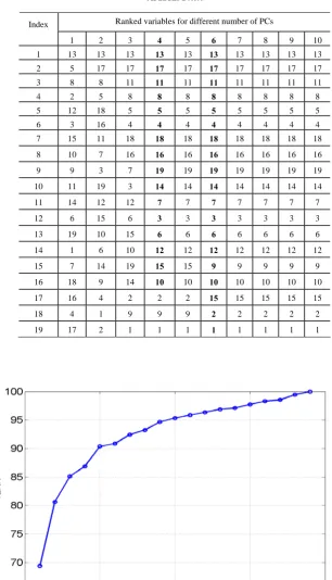
order of the ranked variables becomes stable from p=6. In fact, the order of most ranked variables becomes stable from p=4. The number of PCs could thus be chosen as m=4, rather than m=6. The total error reduction ratio, TERR[d], which refers to what percentage of the overall variation in all the 19 variables can be accounted for by the first d variables in column 4 of Table III, is plotted in Fig. 1. Fig. 1 shows that about 70% overall variation in all the 19 variables can be accounted for by

19 2 1, ,L,

x y_i= T_i

} { 13

1 x

S = , 81% by , 85% by

, 87% by , and 90% by

} , { 13 17

2 x x

S = }

, , { 13 17 11

3 x x x

S = S4={x13,x17,x11,x8} S5 ={x13,x17,x11,x8,x5}, etc.

Note that for the same alate adelges data set, different criteria and different algorithms may lead to different

subsets [Jolliffe 2000]. The subset , selected by MSOLS algorithm here is identical to that

selected by the method B4 (a PCA based algorithm) [Jolliffe 1973]. Compared with other methods, the subset

selected by B4 is considered to be the best in all subsets of three variables [Jolliffe 2000]. }

, , { 13 17 11

3 x x x

S =

}

,

,

{

13 17 11

3

x

x

x

TABLE III

RANKED VARIABLES OBTAINED BY CONSIDERING DIFFERENT NUMBER OF PCS FOR THE ALATE

ADELGES DATA

Ranked variables for different number of PCs Index

1 2 3 4 5 6 7 8 9 10

1 13 13 13 13 13 13 13 13 13 13

2 5 17 17 17 17 17 17 17 17 17

3 8 8 11 11 11 11 11 11 11 11

4 2 5 8 8 8 8 8 8 8 8

5 12 18 5 5 5 5 5 5 5 5

6 3 16 4 4 4 4 4 4 4 4

7 15 11 18 18 18 18 18 18 18 18

8 10 7 16 16 16 16 16 16 16 16

9 9 3 7 19 19 19 19 19 19 19

10 11 19 3 14 14 14 14 14 14 14

11 14 12 12 7 7 7 7 7 7 7

12 6 15 6 3 3 3 3 3 3 3

13 19 10 15 6 6 6 6 6 6 6

14 1 6 10 12 12 12 12 12 12 12

15 7 14 19 15 15 9 9 9 9 9

16 18 9 14 10 10 10 10 10 10 10

17 16 4 2 2 2 15 15 15 15 15

18 4 1 9 9 9 2 2 2 2 2

[image:14.595.139.446.113.648.2]

19 17 2 1 1 1 1 1 1 1 1

[image:14.595.131.447.466.679.2]

TABLE IV

RANKED VARIABLES OBTAINED BY CONSIDERING DIFFERENT NUMBER OF PCS FOR THE PIMA INDIANS DIABETES DATA

Ranked variables for different number of PCs Index

1 2 3 4 5 6 7 8

1 2 2 2 2 2 2 2 2

2 5 5 5 5 5 5 5 5

3 3 8 8 8 8 8 8 8

4 6 4 4 4 4 4 4 4

5 8 3 3 3 3 3 3 3

6 4 6 6 6 6 6 6 6

7 1 7 7 7 7 7 7 7

8 0 1 1 1 1 1 1 1

TABLE V

THE TWO CRITERIA SERR AND TERR FOR THE PIMA INDIANS DIABETES TEST DATA SET

SERR[j;d] (%) TERR[d]

(%) Index j

Index

d 1 2 3 4 5 6 7 8

Test data

Training data 1 53.65 100 90.05 59.90 40.54 91.11 66.05 85.66 73.37 73.39 2 54.88 100 90.08 65.04 100 91.11 66.22 86.32 81.71 82.21 3 71.13 100 92.25 65.35 100 92.07 67.09 100 85.99 85.26 4 71.25 100 92.96 100 100 93.58 68.98 100 90.85 90.13 5 71.26 100 100 100 100 94.85 69.61 100 91.97 91.33 6 71.33 100 100 100 100 100 70.28 100 92.71 92.09 7 71.34 100 100 100 100 100 100 100 96.42 96.09

8 100 100 100 100 100 100 100 100 100 100

4.3 Example 3– The Pima Indians Diabetes data

The pima indians diabetes (PID) data is taken from UCI Machine Learning Repository [Newman et. al 1998].

The PID data set comprises 8 individual features, measured with 768 samples, where the first 500 samples were

used for training and the remaining 268 samples were used for testing. The objective here is to rank the 8

features used in the 500 8 data set. Denote the 8 features by× x₁,x₂,L,x₈.

Similar to Example 1, the significance of the 8 features were detected and ranked by performing the MSOLS

algorithm on a different number of PCs, and the associated results are shown in Table IV, where the number zero

in the 2nd column means that only 7 features are required to represent the first PC. It is clear from Table IV that

the number of PCs to be considered for subset selection is 2. The most significant feature select by MSOLS is ,

referring to the plasma glucose concentration at 2 hours in an oral glucose tolerance test. This feature has been

employed as one of the main criteria by World Health Organization (WHO) for diabetes diagnosis. The result

here just reflects the fact that is significant for diabetes diagnosis.

2 x

The values of SERR[j;d] with respect to the PID test data set are shown in Table V, where the element of SERR in the dth row and jth column indicates what percentage of the variation in the jth variable can be accounted for by the first d variables in column 2 of Table V. The total error reduction ratio, TERR[d], for both the training data set and the test data set are also listed in Table V.

j

x

5. Conclusions

A new learning scheme has been proposed for feature ranking and subset selection. By treating the first

principal components as the response variables and all the candidate features as the predictor variables, the

problem for feature ranking and subset selection can be viewed as a special case of variable detection and subset

selection in multiple linear regression analysis. The new MSOLS algorithm can thus be applied to detect and

rank the features according to the capability to represent the first few PCs. The selected feature subset can be

evaluated by the total error reduction ratio (TERR), which refers to what percentage of the overall variation in all

the features can be accounted for by a selected subset, and which can be used as a criterion to indicate how many

features (variables) need to be included in the subset. Unlike principal components, which carry no clear

physical meaning, variables (features) selected using MSOLS are physically interpretable. The applicability and

usefulness of the new MSOLS algorithm and associated learning scheme for feature (variable) ranking and

subset selection have been demonstrated using results from several examples for both artificial and real data sets,

including the three examples given in Section 4.

Appendix A –The MSOLS algorithm

In the following, are the data vectors associated with the (n+1) candidate variables, are the columns of the matrix X

n x x x0, 1,L,

~

) 1 ( 2

1, ,L, mn+ defined by (3); is the significant variable selected at the

rth step (r=1,2 …) .

r z

The MSOLS algorithm:

Step 1: Set I1={1,L,L}; L=m(n+1); for j=1 toL

_j = _j;

) )( (

) ( ] [ err

2 )

1 (

j T

j T

j T

j

y y

y

=

; {if T_{j j} <

δ

,set err(1)[j]=0}; end for

]} [ err { max arg (1)

1

1

k

I k∈

=

l ; mod( 1, 1);

0

1 = l n+

l

] [ err ] 1

err[ 1

) 1 ( _l

= ; serr[1]=err[1];

; ; { : ismultipleof and 1};

0 1

1= l l l l∈I

1

1 l

q = 0

1 1 x_l

z =

2 ≥ r Step r, :

forr=2 to n+1

Ir =Ir−1\ r−1; for j∈I_r

∑

−

=

− = 1

1

r

k

k k T k

k T

j j

j q

q q

q

) )( (

) ( ] [ err

2 )

(

j T

j T

j T r _j

y y

y

=

; {if T_{j j}<

δ

,set err(r)[j]=0}; (29) end for ( end loop for j )

={arg( <

δ

)};

∈ j

T j I j r

r

J I_r =I_r\J_r; (30) ]}

[ {err max

arg (r) k

I k r

r

∈

=

l ; l0_r =mod(l_r,n+1) ;

] [ err ] [

err r = (r) l_r ;

∑

;

=

= r

k

k r

1

] [ err ]

[ serr

; ; _r ={l:lismultipleofl0_randl∈I_r};

r

r l

q = 0

r

r xl z =

end for (end loop for r )

The MSOLS algorithm provides an effective tool for selecting significant variables for a multiple regression with

an iterative stepwise way. Variables are selected step by step, one variable at a time. Most numerical ill

conditioning can be avoided by eliminating the candidate variables for which are less than a

predetermined threshold

j j T

δ

, say

δ

=10−τ with

τ

≥10(Eqs. (29), (30)). If required, the selection procedure can be terminated at any step when SERR[r] satisfies some specified conditions. This algorithm can be applied to not only the normal cases, where the number of features is smaller than the number of training samples ( ), but

also the cases where the number of features is much larger than that of training samples ( ). The

applications of MSOLS algorithm is not restricted to variable selection in linear regression, it can be used to

select significant model terms for any linear-in-the-parameters models.

N n<

N n≥

Acknowledgements

The authors gratefully acknowledge that this work was supported by EPSRC (UK).

References

S. A. Billings, S. Chen, and M. J. Korenberg, “Identification of MIMO non-linear systems suing a forward regression orthogonal estimator,” Int. J. Control, vol. 49, pp.2157-2189, June 1989.

M. A. Carreira-Perpinan, “Continuous latent variable models for dimensionality reduction and sequential data reconstruction,” Ph.D. dissertation, Dept Computer Science, Univ. Sheffield, Sheffield, U.K., 2001.

S. Chen, S. A. Billings, and W. Luo, “Orthogonal least squares methods and their application to non-linear system identification,” Int. J. Control, vol. 50, pp.1873-1896, Nov.1989

I. K. Fodor, “A survey of dimension reduction techniques,” http://www.llnl.gov/CASC/sapphire/pubs , 2002. nd

S. Haykin, Neural networks: A Comprehensive Foundation (2 ed.). New York: Prentice Hall, 1999. A. K. Jain, R. P. W. Duin, and J. Mao, “Statistical pattern recognition: a review,” IEEE Trans. Pattern Anal.

Machine Intell., vol. 22, pp. 4-37, Jan. 2000.

J. N. R. Jeffers, “Two case studies in the application of principal component analysis,” Appl. Statist., vol. 16, no. 3, pp. 225-236, 1967.

I. T. Jolliffe, “Discarding variables in a principal component analysis. I: artificial data.” Appl. Statist., vol. 21, no. 2, pp. 160-173, 1972.

I. T. Jolliffe, “Discarding variables in a principal component analysis. II: real data.” Appl. Statist., vol. 22, no. 1, pp. 21-31, 1973.

R. Kohavi and G. H. John, “Wrappers for feature subset selection,” Artif. Intell., vol. 97, no.1-2, pp. 273-324, Dec 1997.

M. Korenberg, S. A. Billings, Y. P. Liu, and P. J. McIlroy, “Orthogonal parameter estimation algorithm for

non-linear stochastic systems,” Int. J. Control, vol. 48, no. 1, pp. 193-210, July 1988,

W. J. Krzanowski, “Selection of variables to preserve multivariate data structure using principal components,”

Appl. Statist., vol. 36, no. 1, pp. 22-33, 1987.

K. Z. Mao, “Identifying critical variables of principal components for unsupervised feature selection,” IEEE Trans. Syst., Man, Cybern., B, Cybern, vol. 35, no. 2, pp. 339-344, April 2005.

G. P. McCabe, “Principal variables,” Technometrics, vol. 26, no. 2, pp. 137-144, May 1984.

D. J. Newman, S. Hettich, C. L. Blake, and C. J. Merz, UCI Repository of Machine Learning Databases, [ http://www.ics.uci.edu/~mlearn/MLRepository.html ]. Irvine, CA: Univ. California, Dept. Inform. Comput. Sci., 1998.

E. Oja, Subspace methods of Pattern Recognition. Letchworth, England: Research Studies Press, 1983.

P. Pudil, J. Novovicova, and J. Kittler, “Floating search methods in feature selection,” Pattern Reconit. Lett., vol. 15, no. 11, pp. 1119-1125, Nov 1994.

A. R. Webb, Statistical Pattern Recognition (2nd ed.). New York: Wiley, 2002.