On the Size and Recovery of Submatrices of Ones
in a Random Binary Matrix
Xing Sun XING [email protected]
Merck Research Laboratories 351 N Sumneytown Pike
North Wales, PA 19454-2505, USA
Andrew B. Nobel [email protected]
Department of Statistics and Operation Research University of North Carolina at Chapel Hill Chapel Hill, NC 27599-3260, USA
Editor: Nicolas Vayatis
Abstract
Binary matrices, and their associated submatrices of 1s, play a central role in the study of random bipartite graphs and in core data mining problems such as frequent itemset mining (FIM). Moti-vated by these connections, this paper addresses several statistical questions regarding submatrices of 1s in a random binary matrix with independent Bernoulli entries. We establish a three-point concentration result, and a related probability bound, for the size of the largest square submatrix of 1s in a square Bernoulli matrix, and extend these results to non-square matrices and submatrices with fixed aspect ratios. We then consider the noise sensitivity of frequent itemset mining under a simple binary additive noise model, and show that, even at small noise levels, large blocks of 1s leave behind fragments of only logarithmic size. As a result, standard FIM algorithms, which search only for submatrices of 1s, cannot directly recover such blocks when noise is present. On the positive side, we show that an error-tolerant frequent itemset criterion can recover a submatrix of 1s against a background of 0s plus noise, even when the size of the submatrix of 1s is very small.1
Keywords: frequent itemset mining, bipartite graph, biclique, submatrix of 1s, statistical
signifi-cance
1. Introduction
In many situations, the data obtained from a standard numerical experiment can be represented by a rectangular matrix, whose columns correspond to subjects or samples, and whose rows cor-respond to variables or features measured for each subject. In a number of important cases, the measured features can take one of two values, and the resulting data can be represented as a bi-nary matrix. Prominent examples include data mining tasks such as frequent pattern mining, single nucleotide polymorphism (SNP) data obtained from inbred strains having two allelic variants, and quantized versions of continuous measurements.
The initial analysis of large data sets (typically involving many features and small to moderate numbers of samples) is often exploratory, reflecting the increasing use of such data for hypothesis generation, as well as more traditional hypothesis testing. In unsupervised settings, exploratory analysis seeks to identify patterns or other regularities in the observed data that may point to useful (and potentially unknown) associations between variables, samples or both.
The most common form of exploratory analysis is clustering. Clustering algorithms divide the available samples or variables into disjoint groups so that objects in the same group are, in a suitable sense, close together, while objects in different groups are far apart. A natural extension of standard clustering, usually called biclustering or subspace clustering, looks directly for associations between sets of samples and sets of variables. These associations are represented by submatrices of the data matrix.
In the case of binary matrices, the simplest submatrices of interest are constant, with all entries equal to 1. Submatrices of this sort play a key role in data mining applications, and arise naturally in the study of bipartite graphs (see the discussion below). Motivated in part by these connections, this paper considers the extremal properties of submatrices of 1s in a random binary matrix, and considers the recovery of such submatrices in the presence of noise. More specifically, our analyses are based on a model in which the entries of the principal matrix, and the noise, respectively, are independent Bernoulli(p)random variables. We provide significance bounds for the size of subma-trices of 1s under the Bernoulli null hypothesis, and use these to establish limits on the performance of standard data mining methods in the presence of Bernoulli noise. In the same context, we es-tablish several results on the precise asymptotic size of maximal submatrices of 1s, extending to the setting of bipartite graphs earlier work of Bollob´as and Erd˝os (1976) and Matula (1976) on the size of maximal cliques in random graphs. Lastly, we establish finite sample and asymptotic results concerning the recovery of all-1s submatrices in the presence of noise.
1.1 Overview
Connections between binary matrices, frequent itemset mining, and bipartite graphs are dis-cussed in the next section. Section 3 is devoted to the size of the largest square submatrix of 1s in a random binary matrix. Extensions to non-square matrices are described in Section 4. Section 5 contains a short simulation study that supports our theoretical bounds in a non-asymptotic setting. Section 6 is devoted to the noise sensitivity of frequent itemset mining and the recoverability of block structures in the presence of noise.
2. Motivation and Background
An m×n binary matrix is an indexed family X={xi,j: i∈[m],j∈[n]}where xi,j∈ {0,1}and
[k]denotes the set {1, . . . ,k}. A submatrix of X is a sub-family U ={xi,j : i∈A,j∈B} where
A⊆[m]and B⊆[n]; the Cartesian product C=A×B will be called the index set of U , and we will write U =X[C]. When no ambiguity will arise, the index set C itself will be referred to as a submatrix of X .
2.1 Frequent Itemset Mining
subspace clustering (Agrawal et al., 1998; Cheng and Church, 2000; Tanay et al., 2002) remain ac-tive areas of research. A discussion of FIM and related methods can be found in Hand et al. (2001), Goethals (2003), Madeira and Oliveira (2004) and Tanay et al. (2005).
In the frequent itemset problem, the available data is described by a list S={s1, . . . ,sn}of items
and a set T ={t1, . . . ,tm} of transactions. Each transaction ti consists of a subset of the items in
S. If S contains the items available for purchase at a store, then ti represents a record of the items
purchased during the ith transaction, without multiplicity. The goal of FIM is to identify every (maximal) set of items that appear together in more than k transactions, where k≥1 is a threshold that quantifies “frequent”. The data for the FIM problem can readily be represented by an m×n binary matrix X , with entry xi,j=1 if transaction ti contains item sj, and xi,j=0 otherwise. In this
form the FIM problem can be stated as follows: given X and k≥1, find every submatrix of 1s in X having at least k rows, and report the associated set of columns. If the threshold k is allowed to vary, then FIM algorithms essentially seek to find every maximal submatrix of 1s in the data matrix X .
The ongoing application of FIM to large data sets for the purposes of exploratory and related analyses raises a number of natural statistical questions, which we address below in the general setting of random binary matrices. One natural question is how to assign a nominal significance value to the discovery of a moderately sized submatrix of 1s in a large data matrix, accounting for the obvious issue of multiple comparisons arising in this case. Another question is how standard FIM methods perform in the presence of noise, a common feature of many high-throughput measurement technologies. The third question is how one can recover a submatrix of 1s embedded in a larger matrix of 0s when noise is present.
2.2 Bipartite Graphs
Binary matrices are in one to one correspondence with bipartite graphs. An m×n binary matrix X can be viewed as the adjacency matrix of a graph G= (V,E), where the vertex set V of G is the disjoint union of two sets V1 and V2, with |V1|=m and |V2|=n, corresponding to the rows and
columns of X , respectively. There is an edge(i,j)∈E between vertices i∈V1 and j∈V2 if and
only if xi,j=1; there are no edges between vertices in V1or vertices in V2. A submatrix U of X with
index set C=A×B corresponds to the subgraph G0 of G induced by the vertex set A∪B. If every entry of U is equal to one, then there is an edge(i,j)between every pair of vertices i∈A and j∈B, and G0is then a complete bipartite subgraph of G. Thus maximal submatrices of 1s in X correspond to bicliques in G. This connection is the basis for the biclustering algorithm of Tanay et al. (2002).
It is known (cf., Garey and Johnson, 1979; Hochbaum, 1998; Peeters, 2003) that the problem of finding a biclique with the largest number of edges in a given bipartite graph G is NP-complete, and thus the same is true of the general frequent itemset problem with no restriction on the threshold k. Several approximate methods (Hochbaum, 1998; Dawande et al., 2001; Mishra et al., 2004) have been proposed for finding large bicliques in bipartite graphs in polynomial time. Mishra et al. (2004) show that the results provided by their randomized algorithm overlap a large fraction of the largest bicliques with high probability.
3. Largest Submatrices of 1s: Square Case
In this section we study the size of the largest square submatrix of 1s in a square binary matrix whose entries are independent Bernoulli(p)random variables. Non-square matrices and submatri-ces are considered in Section 4.
Definition: Let Z={zi,j : i,j≥1} be an infinite array of independent binary random variables
with P(zi,j =1) =p=1−P(zi,j =0), where the probability p∈(0,1) is fixed. For n≥1, let
Zn={zi,j: 1≤i,j≤n}.
Thus Zn is an n×n binary random matrix comprising the “upper left corner” of the collection {zi,j}. This definition allows us to make almost-sure type statements concerning the asymptotic
behavior of functions of Zn.
Definition: Given a binary matrix X , let M(X)be the largest k such that there exists a k×k submatrix of 1s in X . Note that M(X)is invariant under row and column permutations of X .
From a statistical point of view, the random matrix Znfollows a simple null model under which
the observed binary data matrix has no special structure, and M(·)acts as a natural test statistic with which to detect departures from the null. Our analysis begins with a bound on the probability that M(Zn) exceeds a fixed integer k≥1. We follow a standard first moment argument (cf., Alon and
Spencer, 1991).
Fix n for the moment, and for each 1≤k≤n let Ukbe the number of k×k submatrices of ones
in Zn. Then, letting S={C=A×B : A,B⊆[n],|A|=|B|=k}, we may write
Uk =
∑
C∈SI{all entries of Zn[C]are 1}
from which it follows that
EUk = |S| ·P(all entries of Zn[C]are 1) =
n k
2
pk2.
By Markov’s inequality and the previous display,
P(M(Zn)≥k) =P(Uk≥1) ≤ EUk =
n k
2
pk2. (1)
We wish to identify an integer knfor which EUkn is approximately equal to one. For values k>kn the rightmost expression in (1) provides an effective means for bounding the probability on the left. Note that EUn=pn
2
<1, and EU1=n2p>1 when n is sufficiently large. Moreover, it is clear from
the definition that Uk+1≤Uk, so that EUk is non-increasing in k. Using the Stirling approximation
of the rightmost expression in (1), define
φn(s) = (2π)−
1 2nn+
1 2s−s−
1
2(n−s)−(n−s)− 1 2 p
s2
2, s∈(0,n).
The quantity φn(k) is an approximation of (EUk)1/2: the ratio φn(k)/(EUk)1/2 is bounded away
from zero and infinity, independent of n,k, and tends to one if k and n−k tend to infinity with n. Let s(n)be any positive real root of the equation
The next lemma shows that s(n)is unique and grows as logarithmically with n.
Lemma 1. When n is sufficiently large, the Equation (2) has a unique root s(n)satisfying logbn<
s(n)<2 logbn, where b=p−1.
Using the bounds of Lemma 1 and some technical but straightforward calculations, one may obtain a simple asymptotic expression for s(n).
Lemma 2. The root s(n)defined by (2) has the form
s(n) = 2 logbn−2 logblogbn+C+o(1)
where b=p−1and C=2 logbe−2 logb2.
The proofs of Lemmas 1 and 2 can be found in Section 7.1. Let k(n) =ds(n)ebe the least integer greater than or equal to s(n). The next proposition provides an upper bound on P(M(Zn)≥k)for
k>k(n). Its proof appears in Section 7.2.
Proposition 1. For eachε>0, when n is sufficiently large, P(M(Zn)≥k(n) +r)≤n−2 r(logbn)2r+ε.
One may obtain a cruder bound, on the probability that M(Zn)is at least 2 logbn+r, in a simpler
fashion by noting that
EUk =
n k
2
pk2 ≤ n
2k
k!2e−
k2log b≤ e2k ln n−k
2ln b
k2 ≤n− 2r
when k≥2 logbn+r. Both the upper bound of Proposition 1 and the definition of s(n)are based on the inequality (1), which follows from a simple union bound on the probability that M(Zn)is at
least k. The union bound is typically quite loose, but it is sufficiently strong in this context to ensure that, for large n, the random variable M(Zn)is close to the threshold s(n). Indeed, it follows from
Proposition 1 and the first Borel Cantelli Lemma that, with probability one, M(Zn)is eventually less
than s(n) +1. Using a more involved second moment argument, one can establish a corresponding lower bound on M(Zn). Together these bounds yield the following result.
Theorem 1. Given any ε>0, with probability one, s(n)−1−ε<M(Zn)<s(n) +ε when n is
sufficiently large.
It follows from Theorem 1 that for large n the size of the largest square submatrix of 1s in Zn
can take one of at most two integer values in an interval of width 1+2εcontaining the number s(n). Indeed, it is shown in the proof of Theorem 1 that there is a sequence of integers{r(n)}close to
{s(n)} such that, with probability one, when n is sufficiently large M(Zn)∈ {rn−1,r(n)}. Thus
M(Zn)exhibits two-point concentration and does not possess a limiting continuous distribution.
The proof of Theorem 1 is given in Section 8. The outline of the proof follows arguments of Bollob´as and Erd˝os (1976), who studied the size of the largest clique cl(Gn)in a random graph Gn
with n vertices, where each edge is included independently with probability p. They showed that for a deterministic function c(n), equal to s(n)up to the constant and lower order terms, eventually almost surely|cl(Gn)−c(n)|<3/2. Matula (1976) independently established a similar result. See
bicliques in balanced bipartite random graphs. (Unbalanced bipartite graphs are considered in the next section.)
Dawande et al. (2001) used first and second moment arguments to show (in our terminology) that P(logbn≤M(Zn)≤2 logbn)→1 as n tends to infinity. Improving these results, Park and
Szpankowski (2005) showed that P((1+ε)logbn≤M(Zn)≤(2−ε)logbn)tends to 1 as n tends to
infinity for any fixed 0<ε<1. Koyut ¨urk et al. (2004) studied the problem of finding dense patterns in binary data matrices. They used a Chernoff type bound for the binomial distribution to assess whether an individual submatrix has an enriched fraction of ones, and employed the resulting test as the basis for a heuristic search for significant bi-clusters. However, the effects of multiple testing are not considered in their assessments of significance. Tanay et al. (2002) assessed the significance of bi-clusters in a real-valued matrix using likelihood-based weights, a normal approximation and a standard Bonferroni correction to account for the multiplicity of submatrices. Use of the normal approximation for individual submatrices leads to subtoptimal bounds in non-Gaussian settings.
3.1 Smallest Maximal Submatrix of 1s
Square submatrices of 1s will occur by chance in a random binary matrix. The largest such submatrix has approximately 2 logbn−2 logblogbn rows. Conversely, one may ask about the size of the smallest maximal square submatrix of 1s. (A square submatrix of 1s is maximal if there is no larger square submatrix of 1s that properly contains it.)
Definition: Let L(Zn)be the smallest k such that there exists at least one k×k maximal submatrix
of 1’s in Zn.
Theorem 1 implies that L(Zn)≤2 logbn. An analysis based on second moment arguments
similar to those used in the proof of Theorem 1 yields the following, tighter bound. The proof can be found in Sun (2007).
Theorem 2. With probability one,
lim
n→∞
L(Zn)
logbn =1.
Bollob´as and Erd˝os (1976) establish a related result on the size of the smallest clique in a random graph. However their proof can not be directly extended to obtain the theorem above. Indeed, an extension of their argument provides a lower bound on the size of the smallest square submatrix of 1s that is not properly contained within a rectangular submatrix of 1s, and the resulting bound is necessarily larger than the one in Theorem 2.
4. Non-Square Matrices
In this section we consider the case where the primary matrix and the target submatrices of 1s may be rectangular, but maintain fixed row/column aspect ratios as the size of the primary matrix grows. Natural analogs of Proposition 1 and Theorem 1 are obtained in this setting. For m,n≥1 define the random matrix Z(m,n) ={zi,j: i∈[m],j∈[n]}.
Definition: Letα>0 andβ>0 be aspect ratios for the primary matrix and target submatrices, re-spectively. Define Mn(Z :α,β)to be the largest k such that Z(dαne,n)contains adβke×k submatrix
The asymptotic behavior of Mn(Z :α,β)is the same as that of Mn(Z :α−1,β−1), so we assume
in what follows thatβ≥1. The analysis of Mn(Z :α,β) proceeds along the same lines as that of
M(Zn). Investigating the value of k for which the expected number ofdβke ×k submatrices of 1s in
Z(dαne,n)is equal to 1, we arrive at the function
s(n,α,β) = 1+β
β logbn−
1+β
β logb
1+β
β logbn
+logbα+C(β) +o(1),
where b=p−1and C(β) =β−1((1+β)log
be−βlogbβ)depends only onβ.
Note that the aspect ratioαof the primary matrix appears only in the constant term of s(n,α,β), and therefore plays only a minor role in what follows. The proofs of Proposition 2 and Theorem 3 below are similar to their analogs in the square case, with additional notation and work required to handle the two aspect ratios, and are omitted. Detailed arguments can be found in Sun (2007).
Proposition 2. Fix aspect ratios α>0, β≥1. For every ε >0, when n is sufficiently large P(Mn(Z :α,β) ≥ ds(n,α,β)e+r) ≤ n−(β+1)r(logbn)(β+1+ε)r.
Remark: When the aspect ratioαof the primary matrix is fixed, it does not play an essential role in the asymptotic behavior of Mn(Z :α,β), which is dominated by higher order factors involving only
the aspect ratioβof the target submatrices. It is natural then to consider a situation in which the aspect ratioαof the primary matrix can increase with n. This might model, for example, the scaling and cost structure of a given high-throughput technology over time. In the case whereα(n) =nγfor someγ>0, the proof of Proposition 2 can be modified to show that
P
Mn(Z : nγ,β) ≥
γ+β+1
β
logbn
≤ n−(β+1)r(logbn)(β+1+ε)r.
On the other hand, one can readily show that ifβ≥1 is fixed and m grows exponentially with n, then Z(m,n) will contain a dβne ×n submatrix of 1’s with probability bounded away from zero. For fixed aspect ratiosαandβone may obtain an asymptotic concentration result for Mn(Z :α,β)
analogous to Theorem 1.
Theorem 3. For fixedα>0 andβ≥1, with probability one|Mn(Z :α,β)−s(n,α,β)| ≤52 when n
is sufficiently large.
Theorem 3 implies that Z(αn,n) contains a submatrix of 1s having aspect ratio β and area
(β+1)log2bn, the latter increasing withβ. Park and Szpankowski (2005) establish a related result, showing that if we do not restrictβ, the aspect ratio of the submatrices, then with high probability the submatrix of 1s in Z(m,n)with the largest area is of size O(n)×ln b or ln b×O(n).
5. Simulation Study
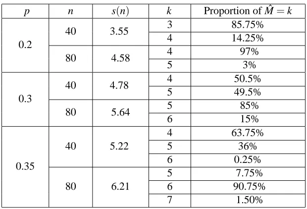
p n s(n) k Proportion of ˆM=k
0.2
40 3.55 3 85.75%
4 14.25%
80 4.58 4 97%
5 3%
0.3
40 4.78 4 50.5%
5 49.5%
80 5.64 5 85%
6 15%
0.35
40 5.22
4 63.75%
5 36%
6 0.25%
80 6.21
5 7.75%
6 90.75%
7 1.50%
Table 1: Distribution of observed ˆM(Zn)based on simulation
the generated random matrix. We recorded the values of ˆM over all simulations and compared these values to the corresponding bounds. Table 1 summarizes the results. Note that in each simulation
−1.5<Mˆ−s(n)<1.
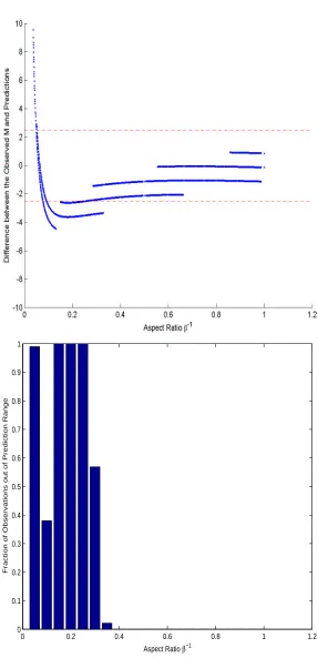
In order to check the theoretical bounds on Mn(Z : 1,β) with β≥1, we considered the 400
random 80×80 matrices with p=0.3 used to evaluate the result for square submatrices above. For each such matrix, we identified all maximal rectangular submatrices of 1s, and recorded the length of both their longer and shorter sides. For eachβ≥1 we defined ˆM(β)to be the largest k such that at least onedβke ×k or k× dβkesubmatrix of 1’s was observed. The difference between ˆM(β)and s(80,1,β)was calculated and is displayed in Figure 1. The x-axes in both panels are equal to 1/β.
The y-axis in the left panel is the difference between ˆM(β) and s(80,1,β), and the y-axis in the right panel is the proportion of simulations which are inconsistent with the theoretical predictions of Theorem 3. Note that even for the moderate matrix size n=80, the theoretical predictions are very accurate when the aspect ratioβis less than 2.5. In these cases, all the observed size lengths are within the range of predicted values.
6. Fragmentation and Recovery in the Presence of Noise
In this section we shift our attention from submatrices of 1s in Znto a setting in which Znplays
the role of binary noise. Formally, we study the additive model
Yn = Xn⊕Zn, (3)
where each matrix is of dimension n×n. The operation⊕is the standard exclusive-or: 0⊕0=
1⊕1=0 and 0⊕1=1⊕0=1. The matrix Xn={xi,j}is a non-random binary matrix that contains
the “true” values of interest, in the absence of noise, and Znis a random binary matrix that acts as
0 0.2 0.4 0.6 0.8 1 1.2 0
0.1 0.2 0.3 0.4 0.5 0.6 0.7 0.8 0.9 1
Aspect Ratio β−1
Fraction of Observations out of Prediction Range
data. Thus the effect of the noise is to randomly flip some of the values of X in Y . The model (3) is the binary version of the standard additive noise model common in statistical inference.
6.1 Noise Sensitivity
Much of the data to which data mining methods are applied is obtained by high-throughput technologies or the automated collection of information from diverse sources with varying levels of reliability. The resulting data sets are often subject to moderate levels of error and noise. Noise can also arise when binary data are obtained by thresholding continuous data, as is sometimes done in microarray analyses. Whatever its source, noise can potentially have serious consequences for frequent itemset methods if they are applied in a direct way to identify submatrices of 1s.
Indeed, this conclusion is already apparent from Theorem 1. If each entry of the target matrix Xnis zero, then Yn=Znand the largest k×k submatrix of ones in Ynhas k≈2 logbn with b=p−1.
At the other extreme, if every entry of Xn is equal to one, then the entries of Yn are independent
Bernoulli(1−p)random variables, and in this case the largest square submatrix of ones in Y has side-length k≈2 logb0n with b0= (1−p)−1. The next result extends this reasoning to any underlying
target matrix Xn.
Proposition 3. Fix 0<p<1/2. Let{Xn}be any sequence of n×n square binary matrices, and
let Yn=Xn⊕Zn. For eachε>0, eventually almost surely(2−ε)logbn<M(Yn)≤2 logb0n, where
b=p−1and b0= (1−p)−1.
Proof of Proposition 3: Fix n and let ˜Wn={w˜i,j} be an n×n binary matrix with independent
entries, defined on the same probability space as{zi,j}, such that
˜ wi,j =
Bern
1−2p 1−p
if xi j=yi j =0
1 if xi j=0,yi j=1
yi,j if xi j=1
where the Bernoulli variable in the first condition is independent of{zi,j}. Define ˜Yn=Yn∨W˜nto be
the entry-wise maximum of Ynand ˜Wn. Then clearly M(Yn)≤M(Y˜n), as any submatrix of ones in Yn
must also be present in ˜Yn. Moreover, the variables ˜yi,j are i.i.d. with P(y˜i,j=1) =1−p, so that we
may regard ˜Ynas a Bern(1−p)noise matrix. It then follows from Theorem 1 that M(Yn)≤2 logb0n
eventually almost surely. To obtain the other inequality, define
ˆ wi,j =
Bern
p 1−p
if xi j=yi j =1
0 if xi j=1,yi j=0
yi,j if xi j=0
and let ˆYn=Yn∧Wˆn be the entry-wise maximum of Yn and ˆWn. It is easy to verify that M(Yn)≥
M(Yˆn), and that the entries in ˆYn are i.i.d. Bern(p). Theorem 1 then implies that M(Yn)≥(2− ε)logbn eventually almost surely.
6.2 Recovery
In light of Proposition 3, it is natural to consider methods for identifying submatrices of 1s that may be contaminated with a certain fraction of 0s. These submatrices correspond, in the data mining and bipartite graph settings, to approximate frequent itemsets and approximate bicliques, respectively. A number of different error-tolerant frequent itemset mining algorithms have been proposed in the literature (Pei et al., 2001, 2002; Yang et al., 2001; Sepp ¨anen and Mannila, 2004; Liu et al., 2005, 2006). Most are based on criteria that require the average of the identified submatrices to be greater than a user specified thresholdτ. One can readily adapt the first moment argument to obtain significance bounds for submatrices with a large fraction of 1s; details can be found in Sun (2007).
Here we consider the simple problem of recovering a (potentially small) submatrix C of 1s em-bedded in a matrix of 0s from a single noisy observation. Proposition 3 shows that one cannot recover C directly using standard frequent itemset mining; instead we consider the Approximate Frequent Itemset (AFI) algorithm developed in Liu et al. (2005).
Definition: Given a binary matrix U with index set C, let F(U) =|C|−1∑(i,j)∈Cui,j be the fraction
of ones in U , or equivalently, the average of the entries of U .
Let ui∗and u∗j denote the rows and columns, respectively, of a given submatrix U .
Definition: Letτ∈[0,1]be fixed. A submatrix U of a binary matrix Y is aτ-approximate frequent itemset (τ-AFI) if each of its rows satisfies F(ui∗)≥τand each of its columns satisfies F(u∗j)≥τ.
Define AFIτ(Y)to be the collection of allτ-AFIs in Y .
The definition above comes from Liu et al. (2005), who presented an algorithm for identifying AFIs in binary matrices.
Let Xnbe an n×n binary matrix that consists of an l×l submatrix of ones having index set C∗,
with all other entries equal to 0. (The rows and columns of C∗ need not be contiguous.) Suppose that Yn=Xn⊕Zn, where Znhas noise level p∈(0,1/2). We wish to recover the index set C∗of the
target submatrix from Yn.
To this end, assume that the noise level p is unknown, but that there is a known upper bound p0
such that p<p0<1/2, and letτ=1−p0be an associated error threshold. We estimate C∗by the
index set of the largest squareτ-AFI in the observed matrix Yn. More precisely, let ˆC be the family
of index sets of square submatrices U∈AFIτ(Yn), and let
ˆ
C =argmax
C∈Cˆ |C|
be the index set of any maximal sized submatrix in ˆC. (The set ˆC contains 1×1 submatrices with
entry 1, so it is non-empty whenever Ynis not identically 0.) Note that ˆC and ˆC depend only on the
observed matrix Yn. Let the ratio
Λ = |Cˆ∩C∗|/|Cˆ∪C∗|
Theorem 4. When n is sufficiently large, for any 0<α<1 such that 8α−1(log
bn+2)≤l we have
P
Λ≤11−+αα
≤ ∆1(l) +∆2(α,l).
Here∆1(l) =2le−
3l(p−p0)2 8p and∆
2(α,l) =2n−
1
4αl+2 logbn, with b=exp{3(1−2 p
0)2/8p}.
Remarks: The second term∆2(α,l)is less than 2n−4/αand is the dominant term in the probability
upper bound if l/ln(n) is large. The logarithmic base b is derived from an upper bound on the tails of the binomial distribution, and is always larger than ˜b=exp{3(1−2 p0)2/8p0}. By a crude
bound,∆1(l)≤∆˜1(l):=e−
√
l when l is sufficiently large. Thus, by replacing b with ˜b and∆ 1(l)
with ˜∆1(l), one obtains a probability bound that does not depend on the unknown parameter p.
As a corollary of Theorem 4, we can also get results in an asymptotic setting. Suppose that
{Xn: n≥1}is a sequence of square binary matrices, and that Xn contains an ln×ln submatrix Cn∗
of 1s with all other entries equal to 0. Let Yn=Xn⊕Zn, and let Λn measure the overlap between
C∗n and the estimate ˆCn produced by the AFI-based recovery method above. The following result
follows from Theorem 4 and the Borel Cantelli lemma.
Corollary 1. If ln≥8ψ(n)(logbn+2)whereψ(n)→∞as n→∞, then eventually almost surely
Λn ≥
1−ψ(n)−1
1+ψ(n)−1 →1.
Reuning-Scherer studied several recovery problems in his thesis (Reuning-Scherer, 1997). In the case considered here, he calculated the fraction of 1s in every row and every column of Y , and then selected those rows and columns for which these fractions exceeded an appropriate threshold. His algorithm is easily seen to be consistent when l≥nαforα>1/2. However, it is easy to show using the central limit theorem that individual row and column sums alone are not sufficient to recover C∗ when l≤nαforα<1/2. In the latter case, one gains considerable power by directly considering submatrices, and as the result above demonstrates, one can consistently recover Cn∗ if ln/ln(n)→∞.
7. Proofs of Preliminary Results
In this section, we will begin with the proofs of Lemma 1 and Lemma 2 then follow with the proof of Proposition 1.
7.1 Proofs of Lemmas 1 and 2
Proof of Lemma 1: Differentiating logb(φn(s))yields
∂logb(φn(s))
∂s =
1
2(n−s)ln b+logb(n−s)−s−logbs− 1 2s ln b,
which is negative when logbn<s<2 logbn. A routine calculation shows that for 0<s≤logbn,
logbφn(s) = (n+
1
2)logbn−(s+ 1
2)logbs−(n−s+ 1
2)logb(n−s)− s2
2 −
1 2logb2π
≥ s
logb(n−logbn)−s
2−logblogbn
−12logbs−1
when n is sufficiently large. Similarly, for 2 logbn≤s<n,
logbφn(s) ≤ s
logb(n−s)−s
2−logbs
−1
2logbs− 1
2logb2π+2s+ s logbs
2
≤ s
2−logbs 2
−1
2logbs− 1
2logb2π < 0
when n is sufficiently large. Thus for sufficiently large n, there exists a unique solution s(n)of the equationφn(s) =1 with s(n)∈(logbn,2 logbn).
Proof of Lemma 2: Taking logarithms of both sides of the equation φn(s) =1 and rearranging
terms yields
1 2logb
n
n−s+n logb n
n−s−(s+ 1
2)logbs+s logb(n−s)− s2
2 =
logb2π
2 .
Lemma 1 implies that s(n)belongs to the interval(logbn,2 logbn), so we consider the above equa-tion in the case that n>>s. Dividing both sides of the equation by s yields
logb(n−s)−s
2−logbs=−logbe+O( logbs
s ),
which can be rewritten as
logbn−s
2−logblogbn=logb s
logbn−logb n−s
n −logbe+O( logbs
s ). (4)
For each n, define R(n)via the equation
s(n) = 2 logbn−2 logblogbn+R(n).
Plugging this expression into (4), it follows that R(n) =2 logbe−2 logb2+o(1), and the result follows from the uniqueness of s(n).
7.2 Proof of Proposition 1
To establish the bound with r independent of n, it suffices to consider a sequence rnthat changes
with n in such a way that 1≤rn≤n. Fix n for the moment, let l=k(n) +rn, and let Ul be the
number of l×l submatrices of 1s in Zn. Then by Markov’s inequality and Stirling’s approximation,
P(M(Zn)≥l) = P(Ul ≥1) ≤ E(Ul) =
n l
2
pl2 ≤ 2φ2n(l).
A straightforward calculation using the definition ofφn(·)shows that one can decompose the
rightmost term above as follows:
2φ2
where
An(r) =
n−r−k(n)
n−k(n)
−n+r+k(n)+12
, Bn(r) =
r+k(n)
k(n)
−k(n)−21
,
Cn(r) =
n−k(n)
r+k(n) p
k(n)
2
r
, Dn(r) = p
r2
2.
Note that pr·k(n)=o(n−2r(logbn)2r+ε)for any fixedε>0, and thatφ2
n(k(n))≤1 by the
mono-tonicity ofφn(·)and the definition of k(n). Thus it suffices to show that An(r)·Bn(r)·Cn(r)·Dn(r) =
O(1)when n is sufficiently large. To begin, note that for any fixedδ∈(0,1/2), when n is sufficiently large,
Cn(r)
1
r = n−k(n) r+k(n) p
k(n)
2 ≤ n
k(n)p
k(n)
2 ≤ n
(2−δ)logbn
2+δ
2 logbn
n ,
which is less than one. Note that Bn(r)≤1. It only remains to show An(r)·Dn(r) =O(1). Simple
calculations yield that ln An(r)≤r. Consequently, ln(An(r)·Dn(r))≤r−r
2ln b
2 , which is bounded
from above.
8. Proof of Theorem 1
The proof of Theorem 1 is established via a sequence of technical lemmas. Modifying our ear-lier notation slightly, let Uk(n)denote the number of k×k submatrices of 1s in Zn. In what follows
εis a fixed positive number less than 12. Our argument parallels that outlined in Bollob´as (2001). We begin with the following definition.
Definition: For each k≥1, let n0kbe the least integer n such that
EUk(n)≥k3+ε,
and let nk be the largest integer n such that
EUk(n)≤k−3−ε.
Note that nk and n0kexist for sufficiently large k≥1, as EUk(k) =pk
2
≤k−3−ε, EUk(n)is monotone
increasing in n, and EUk(n)→∞as n→∞.
Lemma 3. Let nkand n0kbe defined as above.
a. When k is sufficiently large, n0k<nk+1.
b. When k is sufficiently large, n0k−nk<C1nkkln k for some constant C1>2.
c. limk→∞nk+nk+2−1−nnk+k1 =b
1 2.
Proof of (a): It follows from the definition of nkthat
nk
k
pk22 ≤k−
(3+ε)
2 and
nk+1
k
pk22 ≥k−
(3+ε)
Rearranging terms in the first inequality, and noting that(nk−k)!/nk!≤(nk−k)−k we obtain, in
turn, the inequalities
k(3+2ε)
k! bk22
≤ (n 1 k−k)k
and nk≤b
k
2
k!
k(3+2ε)
1k
+k.
Rearranging the terms in the second inequality of (5), one may establish by a similar argument the inequalities
k(3+2ε) ≥b
k2
2 k!
(n+1)k and nk ≥b
k
2
k!
k3+2ε
1k
−1.
Combining the two bounds on nk above, yields
bk2
k! k−3+2ε
1k
−1≤ nk ≤b
k
2
k! k−(3+2ε)
1k
+k (6)
and the asymptotic relation
nk =b
k
2(k!) 1
k +o(k b k
2). (7)
From the definition of n0k, one can establish in a similar fashion the inequalities
bk2
k! k3+2ε
1k
≤n0k ≤bk2
k! k(3+2ε)
1k
+k+1. (8)
and the asymptotic relation
n0k=bk2(k!)1k+o(k bk2). (9)
The asymptotic expressions for nkand n0k ensure that n0k<nk+1when k is sufficiently large. Proof of (b): It follows from inequalities (6) and (8) that, when k is sufficiently large,
n0k−nk ≤ b
k
2
k! k(3+2ε)
1k
+k+1−
bk2
k! k−3+2ε
1k
−1
≤ bk2
k! k−3+2ε
1k
(k3+kε−1) +k+2
≤ (nk+1)(k
3+ε
k −1) +k+2
< nkC1
log k k .
for some constant C1>2. The third inequality above is a consequence of (6), while the last
inequal-ity follows from the fact that x−1<2 ln x for x close to 1.
Proof of (c): It follows from Equations (7) and (9) that
nk+1
nk
=b12 +o(1) and nk+2
nk+1
=b12+o(1).
Therefore, as k tends to infinity,
nk+2−nk+1
nk+1−nk
=
nk+2
nk+1−1
1− nk
nk+1
This completes the proof of Lemma 3.
We now continue the analysis of Uk(n). The second moment argument used below requires
bounds on the ratio
g(Uk(n)):=Var(Uk(n))/(EUk(n))2
which arises in a standard Chebyshev bound on the tails of Uk(n). Letting
S={C=A×B : A,B⊆[n],|A|=|B|=k}
be the family of index sets of k×k submatrices, we see that
Uk(n)2 =
∑
C,C0∈SI{each entry of Zn[C]and Zn[C0]is 1}.
From the last display one may readily derive that
EUk(n)2 = k
∑
l=1
n k k l
n−k k−l
k
∑
r=1
n k k r
n−k k−r
·p2 k2−lr,
where the indices k and l indicate the number of rows and columns, respectively, that the submatrices C and C0have in common. As EUk(n) = nk
2
pk2, we find that
g(Uk) = k
∑
l=0 k
∑
r=0 k l
n−k k−l
n k k r
n−k k−r
n k
b
lr −1,
where b=p−1. Recall that 0<ε<12 is fixed.
Lemma 4. There exists a constant C0>0 such that g(Uk(n))≤C0k−1−εfor every sufficiently large
k and every n0k≤n≤nk+1.
Proof of Lemma 4: To begin, note that
g(Uk(n)) = k
∑
l=0 k
∑
r=0 k l
n−k
k−l
n k k r
n−k
k−r
n k
(b
lr −1)
=
k
∑
l=1 k
∑
r=1 k l
n−k k−l
n k k r
n−k k−r
n k
(b
lr−1)
< k
∑
l=1 k
∑
r=1 k l
n−k
k−l
n k k r
n−k
k−r
n k b lr ≤ k
∑
r=1 k r
n−k
k−r
n k
(b
r2/2
)
!2
,
where the last inequality follows from the fact that blr≤bl2+r22 . Thus it suffices to show that
k
∑
r=1
h(r) =O(k−1/2−ε/2) where h(r):=
k r
n−k k−r
n k
b
r2/2. (10)
If n≥n0k, then by inequality (8), n≥bk2
k! k3+2ε
1k
it follows from the assumption that n≥n0k and the definition of n0k that nkpk22 =pEUk(n)≥
p
EUk(n0k)≥k3/2+ε/2. Using these inequalities, one can upper bound h(1), h(k−1) and h(k) as
follows:
h(1) =
k 1
n−k k−1
n k
b
1/2 = b1/2k2(n−k)!(n−k)! (n−2k+1)!n! <
b1/2k2 n−k =O(k
2b−k/2),
h(k−1) = k(nn−k)
k
b
k2
2−k+ 1
2 ≤ knb 1 2−k
p
EUk(n)
= O
k−1/2−ε/2b−k(1−η)/(2−η)
,
h(k) = b
k2 2 n k = 1 p
EUk(n)
≤ k−3/2−ε/2,
In order to establish inequality (10), it therefore suffices to verify that when k is sufficiently large,
h(r)≤h(1) +h(k−1) (11)
for any 1<r<k−1. To this end, note that
h(r+1)
h(r) =
(k−r)2br+1 2
(r+1) (n−2k+r+1).
When r≤ 13k, the inequality k≤2 logbn implies that h(r+1)
h(r) ≤
bk2bk3
n−2k+r+1 ≤
bk2n23
n−2k+r+1 <1.
When 23k≤r<k−1 the inequality k≥(2−η)logbn with 0<η<1/2 implies that h(r+1)
h(r) ≥
b2k3
k(n+r+1) ≥
n2(23−η)
k(n+r+1) >1.
In order to show inequality (11), it now suffices to show that h(r) is log-convex for all integer r∈[dk
3e −1,d 2k
3e]. Since for r∈[d k 3e −1,d
2k 3e],
ln h(r) =ln h(dk
3e −1) +
r−dk
3e
∑
i=0
ln h(d
k 3e+i)
h(dk
3e+i−1) ,
it is equivalent to show that h(hr(+r)1) is monotone increasing. To verify this, note that the derivative ∂[h(r+1)/h(r)]/∂r is equal to
b2r2+1(k−r)
(r+1) (n−2k+r+1)
−2(r+1) (n−2k+r+1)−(k−r) (2r+n−2k+2)
(r+1) (n−2k+1) + (k−r)ln b
.
When k is sufficiently large and nk>r, the sum of the leading terms on the last expression above is
−2n(r+1)−(k−r)n+ (k−r) (r+1)n ln b = n(−r2ln b+kr ln b−k−r+ (k−r)ln b−2).
By plugging in r=k
3 and r= 2k
3, it is not hard to check that this quadratic form in r is positive for
any r∈[dk 3e −1,d
2k
Lemma 5. With probability one, when k is sufficiently large, M(Zn) =k whenever n0k≤n≤nk+1. Proof of Lemma 5: By the definition of nk+1and Markov’s inequality, when n≤nk+1,
P(M(Zn)>k)≤ E(Uk+1(n))≤E(Uk+1(nk+1))≤(k+1)−3−ε.
Moreover, Chebyshev’s inequality and Lemma 4 together imply that for n0k≤n≤nk+1,
P(M(Zn)<k) =P(Uk(n) =0) ≤
Var(Uk(n))
(EUk(n))2 ≤
C0·k−1−ε.
As M(Zn)is monotone increasing with n, the previous bounds yield
∑
k≥1
P
nk+1
[
n=n0k
{M(Zn)6=k}
≤
∑
k≥1
PM(Zn0
k)<k
+
∑
k≥1
P M(Znk+1)≥k
≤
∑
k≥1
C0·k−1−ε+
1 k3+ε
<∞.
and the result follows from the Borel-Cantelli lemma.
Proof of Theorem 1: From Lemma 5 we may deduce that with probability one M(Zn)is eventually
equal to one of two possible consecutive integers, whose values depend only on n. It follows from their definition that nk <n0k, and by Lemma 3 both integers tend to infinity as k tends to infinity.
Therefore for every k greater than or equal to some k0we have ... <nk<n0k<nk+1<n0k+1< ....
Thus for all n≥nk0 there exists a unique integer k (depending on n) such that n0k ≤n≤nk+1 or
nk<n<n0k. In the former case, Lemma 5 implies that M(Zn) =k when n is sufficiently large. In
the latter case, Lemma 5 and the monotonicity of M(Zn)in n imply that
k−1=M(Znk)≤M(Zn)≤M(Zn0k) =k,
when n is sufficiently large, so that M(Zn)can take one of at most two possible values, k−1 and k.
It remains to connect M(Zn)and s(n). To begin, let n be such that n0k≤n≤nk+1for some k≥k0.
Then by definition of nk+1and s(n),
(1+o(1))φn(k+1) = (EUk+1(n))1/2 ≤(EUk+1(nk+1))1/2 ≤k−3/2−ε/2 <1= φn(s(n)).
Asφn(k) is monotone decreasing in k, we conclude that s(n)<k+1 when n is sufficiently large.
Similarly,
(1+o(1))φn(k) = (E Uk(n))1/2 ≥(E Uk(n0k))1/2 ≥k3/2+ε/2 >1 =φn(s(n)),
which implies s(n)>k. Thus, with probability one, when n is sufficiently large
Suppose now that nk ≤n≤n0k. Then s(nk) ≤s(n)≤s(n0k) and the arguments above show that
s(nk)<k and s(n0k)>k. We establish that s(n0k)−s(nk) =o(1). To this end, note that
0<s(n0k)−s(nk) =2 logb
n0k nk−
2 logblogbn 0 k
logbnk
+o(1) ≤2 logbn 0 k
nk
+o(1)
as logbn0k
logbnk >1. It therefore suffices to show that logb
n0k
nk =o(1), but this follows from part (b) of Lemma 3. Putting the bounds above together with Lemma 5, we find that with probability one, when n is sufficiently large
nk≤n≤n0k implies k−ε<s(n)<k+εand M(Zn)∈ {k−1,k}. (13)
Combining relations (12) and (13) yields the desired bound on M(Zn).
9. Proof of Theorem 4
The following lemmas are used in the proof of Theorem 4. Lemma 6 shows that|Cˆ|is greater than or equal to |C∗|with high probability, and Lemma 9 shows that ˆC can only contain a small proportion of entries outside C∗. Lemma 7 and Lemma 8 are used in the proof of Lemma 9.
Lemma 6. Under the conditions of Theorem 4, P |Cˆ|<l2
≤∆1(l).
Proof of Lemma 6: Let u1∗, ...,ul∗be the rows of C∗in Y , and let V be the number of rows satisfying
F(ui∗)<τ=1−p0. By the union bound and a standard bound (Devroye et al., 1996) on the tail of
the binomial distribution, P(V≥1)≤l·e−
3l(p−p0)2
8p . The same inequality holds for the number V0of
columns u∗jof C∗such that F(u∗i)<1−p0. Since{|Cˆ|<l2=|C∗|} ⊂ {C∗∈/AFIτ(Y)} ⊂ {V ≥
1} ∪ {V0≥1}, we have
P{|Cˆ|<l2} ≤ P(V ≥1) +P(V0≥1) ≤ 2le−8p3l(p−p0)2 = ∆
1(l).
Lemma 7. Given 0<τ0<1, if there exists a k×r binary matrix V such that F(V)≥τ0, then there
exists a v×v submatrix U of V such that F(U)≥τ0, where v=min{k,r}.
Proof of Lemma 7: Without loss of generality, assume v=k≤r. Order the columns of V in descending order of the number of 1s they contain. If U contains the first v columns in this order, then F(U)≥τ0.
Lemma 8. Let 1<γ<2. Let W be a binary matrix, and let R1and R2be two square submatrices
of W such that (i)|R2|=k2, (ii)|R1\R2|>kγand (iii) R1∈AFIτ(W). Then when k is sufficiently
large there exists a square submatrix D⊂R1\R2such that|D| ≥k2γ−2/16 and F(D)≥τ.
Proof of Lemma 8: The result is clearly true if R1∩R2= /0, so we assume that R1and R2overlap
after suitable row and column permutations, R1\R2 can be expressed either as a single maximal
rectangular submatrix W1, or as the union of two overlapping maximal rectangular W1∪W2. (A
Case 1: R1 and R2 overlap on an edge. Suppose that the difference R1\R2 can be expressed as
a single rectangular submatrix W1. Let l1 and l2 be the side lengths of W1. In this case, the side
length of the square submatrix R1 must be less than k, and consequently max(l1,l2)≤k. Since |R1\R2| ≥kγ, it follows that min(l1,l2)≥kγ−1. As R1∈AFIτ(W)we have F(W1)≥τ. By Lemma
7, there exists a v×v submatrix D of W1such that F(D)≥τand v≥min(l1,l2)≥kγ−1.
Case 2: R1 and R2 overlap on a corner. Suppose R1\R2 is the union W1∪W2 of two maximal
rectangular submatrices. Then clearly max(|W1|,|W2|)≥ |R1\2R2|. Without loss of generality, we
assume that|W1| ≥ |W2|. As R1∈AFIτ(W), F(W1)≥τ, and it suffices by Lemma 7 to show that the
length of the shorter side of W1is greater than kγ−1/4.
Let l1 ≤l2 be the side lengths of W1 and suppose for the moment that l1<kγ−1/4. Then
l2>2k|R1γ−\1R/24| and|R1|=l22≥| R1\R2|2
k2γ−2/4, and it follows that
|R1\R2| ≥ |R1| − |R2| > |R1\R2| 2
k2γ−2/4 −k 2.
Dividing both sides of the previous inequality by|R1\R2|and using the assumption |R1\R2| ≥kγ
yields
1 > |R1\R2|
k2γ−2/4−
k2 |R1\R2| ≥
4k(2−γ)−k(2−γ) = 3k(2−γ).
When k is sufficiently large, this yields a contradiction and completes the proof.
Lemma 9. LetA be the collection of C∈Cˆsuch that|C| ≥l2 and |C∩C∗c|
|C| ≥α, whereα∈(0,1) satisfies l≥8α−1(log
bn+2). Let A be the event thatA 6=/0. If n is sufficiently large,
P(A) ≤ ∆2(α,l).
Proof of Lemma 9: Recall that|C∗|=l2. If C∈A then C∈AFI1−p
0(Y)and
|C\C∗| = |C| · |C∩C ∗c
| |C| ≥ l
2
· α = lγ
where γ = 2+loglα. Thus, by Lemma 8 there exists a v×v submatrix D of C\C∗ such that F(D) ≥ 1−p0and v ≥ α4l. It follows that
max
c∈Cˆ
Mτ(C∩C∗c) ≥ v ≥ αl
4 ,
whereτ=1−p0and Mτ(X)is size of the largest square submatrix with average greater thanτin a
given matrix X .
Let W =W(Y,C∗) be an n×n binary random matrix, with wi j =yi j if(i,j)∈/C∗, and wi j ∼
Bern(p)otherwise. Then it is clear that
Mτ(W) ≥ max
c∈Cˆ
Mτ(C∩C∗c) ≥ αl
When n is sufficiently large and l≥8α−1(log
bn+2), we can bound P(A)as follows
P(A) ≤ P(max
c∈Cˆ
Mτ(C∩C∗c) ≥ αl
4 )
≤ P(Mτ(W)≥αl
4 ) ≤ 2n
−(αl/4−2 logb0n), (14)
where b0 =e
3(1−p0−p)2
8p . Note that the last inequality follows from a first moment argument similar
to that in the proof of Proposition 1 and a standard inequality for the tails of the binomial distribu-tion(cf., Problem 8.3 of Devroye et al. 1996). As p0>p, b<b0, and consequently one can bound
the right hand side of inequality (14) by∆2(α,l). For detailed proof of inequality (14), please refer
to Proposition 3.3.1 in Sun (2007).
Proof of Theorem 4: Let E be the event that{Λ≤11−+αα}. It is clear that E can be expressed as the union of two disjoint events E1and E2, where
E1 = {|Cˆ|<|C∗|} ∩E and E2 = {|Cˆ| ≥ |C∗|} ∩E.
One can bound P(E1)by∆1(l)via Lemma 6.
It remains to bound P(E2). By the definition of Λ, the inequality Λ≤ 11−+αα can be rewritten
equivalently as
1+|Cˆ∩C∗
c | |Cˆ∩C∗| +
|Cˆc∩C∗| |Cˆ∩C∗| ≥
1+α
1−α.
When|Cˆ| ≥ |C∗|, one can verify that|Cˆ∩C∗c| ≥ |Cˆc∩C∗|, which implies that
1+|Cˆ∩C∗
c | |Cˆ∩C∗| +
|Cˆc∩C∗|
|Cˆ∩C∗| ≤1+2
|Cˆ∩C∗c|
|Cˆ∩C∗|.
Therefore, E2⊂E2∗, where
E2∗ = {|Cˆ| ≥ |C∗|} ∩
1+2|Cˆ∩C ∗c
| |Cˆ∩C∗| ≥
1+α
1−α
⊂ {|Cˆ| ≥l2} ∩
1+2|Cˆ∩C ∗c
| |Cˆ∩C∗| ≥
1+α
1−α
.
Notice that 1+2|Cˆ∩C∗c| |Cˆ∩C∗| ≥
1+α
1−α implies | ˆ C∩C∗c|
|Cˆ| ≥α. Therefore, by Lemma 9, P(E2∗)≤∆2(α,l). Acknowledgments
References
R. Agrawal, T. Imielinski, and A. Swami. Mining association rules between sets of items in large databases. In Proceedings of the ACM SIGMOD International Conference on Management of data, pages 207-216, 1993.
R. Agrawal, H. Mannila, R. Srikant, H. Toivonen, and A. Verkamo. Fast discovery of association rules. In U. M. Fayyad et. al, editors, Advances in Knowledge Discovery and Data Mining, AAAI Press, Chapter 12, 307-328, 1996.
R. Agrawal, J. Gehrke, D. Gunopulos, and P. Raghavan. Automatic subspace clustering of high dimensional data for data mining applications. In Proceedings of the ACM SIGMOD international conference on Management of data, pages 94-105, 1998.
N. Alon and J. Spencer. The Probabilistic Method. John Wiley. New York, 1991.
B. Bollob´as and P. Erd˝os. Cliques in random graphs. In Mathematical Proceedings of the Cambridge Philosophy Society, 80:419-427, 1976.
B. Bollob´as. Random Graphs. 2nd ed., Cambridge University Press, 2001.
Y. Cheng and G. M. Church. Biclustering of expression data. In Proceedings of the 8th International Conference on Intelligent Systems for Molecular Biology, pages 93-103, 2000.
M. Dawande, P. Keskinocak, J. Swaminathan, and S. Tayur. On bipartite and multipartite clique problems. Journal of Algorithms, 41:388-403, 2001.
L. Devroye, L. Gyorfi, and G, Lugosi. A Probabilistic Theory of Pattern Recognition. Springer, New York, 1996.
M. R. Garey and D. S. Johnson. Computers and Intractability, A Guide to the Theory of NP-completeness. Freeman, San Francisco, 1979.
B. Goethals. Survey on Frequent Pattern Mining.www.adrem.ua.ac.be/˜goethals/software/ survey.pdf.2003.
J. Han, J. Pei and Y. Yin. Mining frequent patterns without candidate generation. In Proceedings of ACM SIGMOD International Conference on Management of Data, pages 1-12, 2000.
D. J. Hand, H. Mannila and P. Smyth. Principles of Data Mining. MIT Press, 2001.
D. S. Hochbaum. Approximating clique and biclique problems. Journal of Algorithms, 29(1):174-200, 1998.
M. Koyut¨urk, W. Szpankowski and A. Grama. Biclustering gene-feature matrices for statistically significant dense patterns. In Proceedings of the 8th Annual International Conference on Re-search in Computational Molecular Biology, pages 480-484, 2004.