This is a repository copy of A compositional stochastic model for real time freeway traffic simulation.
White Rose Research Online URL for this paper: http://eprints.whiterose.ac.uk/82260/
Version: Submitted Version
Article:
Boel, R. and Mihaylova, L. (2006) A compositional stochastic model for real time freeway traffic simulation. Transportation Research Part B: Methodological, 40 (4). 319 - 334. ISSN 0191-2615
https://doi.org/10.1016/j.trb.2005.05.001
[email protected] https://eprints.whiterose.ac.uk/
Reuse
Unless indicated otherwise, fulltext items are protected by copyright with all rights reserved. The copyright exception in section 29 of the Copyright, Designs and Patents Act 1988 allows the making of a single copy solely for the purpose of non-commercial research or private study within the limits of fair dealing. The publisher or other rights-holder may allow further reproduction and re-use of this version - refer to the White Rose Research Online record for this item. Where records identify the publisher as the copyright holder, users can verify any specific terms of use on the publisher’s website.
Takedown
If you consider content in White Rose Research Online to be in breach of UK law, please notify us by
A Compositional Stochastic Model
for Real-Time Freeway Traffic Simulation
Ren´e Boel
a, Lyudmila Mihaylova
∗
,baUniversity of Ghent, SYSTeMS Research Group, B-9052 Zwijnaarde, Belgium
bDepartment of Electrical and Electronic Engineering, University of Bristol,
Merchant Venturers Building, Woodland Road, Bristol BS8 1UB, UK
Abstract
Traffic flow on freeways is a nonlinear, many-particle phenomenon, with complex interactions between vehicles. This paper presents a stochastic model of freeway traf-fic at a time scale and of a level of detail suitable for on-line estimation, routing and ramp metering control. The freeway is considered as a network of intercon-nected components, corresponding to one-way road links consisting of consecutively connected short sections (cells). The compositional model proposed here extends the Daganzo cell transmission model by defining sending and receiving functions explic-itly as random variables, and by also specifying the dynamics of the average speed in each cell. Simple stochastic equations describing the macroscopic traffic behavior of each cell, as well as its interaction with neighboring cells are obtained. This will allow the simulation of quite large road networks by composing many links. The model is validated over synthetic data with abrupt changes in the number of lanes and over real traffic data sets collected from a Belgian freeway.
Keywords– macroscopic traffic models, freeway traffic, stochastic systems, send-ing and receivsend-ing functions
1 Motivation and relation to previous work
Traffic flow on freeways is a complex process with many interacting components and ran-dom perturbations such as traffic jams, stop-and-go-waves, hysteresis phenomena. These perturbations propagate from upstream to downstream road sections (cells) forming
for-ward waves, usually when traffic is light. During traffic jams drivers are slowing down when
they observe traffic congestion in the cell ahead of them, causing upstream propagation of a traffic density perturbation. The development of models capable of capturing these differ-ent interactions between neighboring cells is a challenging task. In (Daganzo, 1994, 1995)
piecewise affine static sending and receiving functions were introduced to describe the
in-teraction between neighboring road cells, and these waves together. This model, called acell
transmission model (CTM)clearly describes the interaction between neighboring road cells.
∗ Corresponding author
Email addresses: [email protected](Ren´e Boel), [email protected]
Since it relies on a sending function depending only on the state of upstream cells, and on a receiving function depending on the state of downstream cells, it is very well suited for the dynamic analysis of large road networks. The CTM model provides an intuitively appealing and easy to tunedeterministicdescription of how the number of vehicles in consecutive cells of a freeway evolves over consecutive time intervals.
In the present paper we develop astochastic compositional model of the evolution of traffic flows on freeways. It is aimed to be applied to on-line prediction algorithms and control strategies (such as ramp metering and adaptive routing) for large freeway networks. The time scale of the traffic control actions requires aggregated models, which describe the dynamics of macroscopic variables such as density and average speed. The size of the network under study brings the necessity of compositionality, robustness. The model allows a lot of flexibility in choosing the time update step size and the cell sizes. These can vary with time depending on the availability of on-line measurements and with the location of the cells (e.g. on the location of sensors), as long as the generic condition is satisfied that “no vehicle can jump over a cell during one time step”.
In order to properly select good control actions, the simulation model must allow predictions of the future costs resulting from the control decisions we envisage. This cost could be, e.g., the average time delay incurred by vehicles crossing the freeway network under study, a delay that will depend on the speed of the vehicles and hence on the congestion over a considered time horizon. The effects of the control actions are to a great extent predetermined by the evolution of the average speed in each cell over time intervals of the order of a few minutes. For these short intervals of time, and for the high average speed of freeway traffic, the inertia of platoons of vehicles adjusting their driving speed to changes in the local traffic density, will not be negligible. Hence, we extend the CTM model with a dynamic equation describing how speed evolves dynamically in each cell of the road network.
The model we propose describes well the interaction between variables in different cells of the freeway network, and the local dynamics in each cell. First results for traffic modelling with this compositional model were reported in (Boel & Mihaylova, 2004; Mihaylova & Boel, 2003). The model allows for parallel processing which can reduce the computational load. It brings the scalability potential of the decentralized architectures and makes predictors and controllers more robust, by avoiding the need for a centralized processing node. It is also flexible because it is easy to update the model when a local change occurs into some parts of the road network: only the description of one or a few cells has to be modified.
a powerful sample-based method with a wide range of applications in science and engineering (Doucet, Freitas, & N. Gordon, 2001; Ristic, Arulampalam, & Gordon, 2004).
The outline of this paper is as follows. Section 2 presents the compositional description of the freeway network under study, and the traffic variables of interest. Section 3 introduces the dynamic model of one component of the freeway traffic network, using stochastic sending and receiving functions of vehicles passing from one cell to the next cell. Section 4 demonstrates the effectiveness of our model comparing synthetic data and real data obtained from Flemish road authorities. Finally, conclusions and ongoing research issues are highlighted.
2 Problem setup and definition of the traffic variables
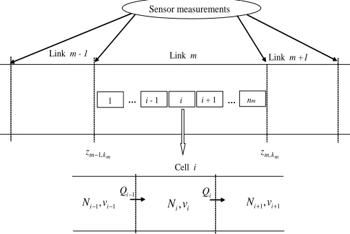
A freeway network can be represented as a sequence of links. A link m is composed of a sequence of cells, numbered from 1 tonm,as indicated in Fig. 1. Each link involves several
lanes in one direction of a freeway, e.g. connecting two major intersections, or important on-or off-ramps. Links are indexed by a numberm,ranging from 1 toM. The lengthLi of each
cell is small enough - typically a few hundred meters - so that the variables describing the traffic behavior at some time instant tk can be assumed approximately uniform inside one
cell. The evolution of the traffic variables in a cell, as measured at an increasing sequence of time instants t0, t1, . . . , tk, . . . , forms the basic building block of our model. The traffic
variables at time tk which the model presented in this paper deals with are:
• the number of vehicles Ni,k in cell i at timetk and
• the average speed vi,k of these Ni,k vehicles at time tk.
The intervals [tk, tk+1) should be small enough to allow accurate modelling (typically less
than 10sec), but not too small so that predictions over time horizons of a few minutes, relevant for the control actions that are envisaged as applications of this model, can be carried out in real time.
Neighboring cells interact with each other because vehicles that are leaving the downstream boundary of celliin a time interval [tk, tk+1) are entering celli+1 via the upstream boundary
1 − i
Q
Cell i
i
Q
1 1, −
− i
i v N
i iv
N , Ni+1,vi+1
m k m
z −1,
Sensor measurements
1 … i - 1 i i + 1 … nm
m k m
z ,
[image:4.595.197.451.571.741.2]Link m - 1 Link m Link m +1
of cell i+ 1 during the same time interval [tk, tk+1). In the equations below we represent
this number of vehicles that enter the cell i+ 1 from cell iduring the time interval [tk, tk+1)
by Qi,k, called the outflow from cell i in time interval [tk, tk+1), or the inflow into cell
i+ 1 (see Fig. 1). Cells 1 andnm are special because their inflow of vehicles at the upstream
boundary, respectively the outflow from the downstream boundary, are interactions with other links, adjacent to link m.
The evolution of the traffic variables within a cell i depends not only on the inflow into cell i, and the outflow from cell i (inflow for cell i+ 1), but also on fixed parameters such as the cell’s length Li, the number of lanes ℓi,k available at time tk, and on parameters of
the speed-density relation, that may vary over time due to uncontrollable or random effects such as weather, accidents, speed limitations.
3 Traffic dynamics for one link
3.1 Updating the number of vehicles in a cell
The evolution of the number of vehicles Ni,k within a cell i measured at consecutive time
instants tk can be expressed by theconservation of vehicles equation:
Ni,k+1 =Ni,k +Qi−1,k−Qi,k, (1)
where the number of vehicles Qi,k crossing the boundary between cells i and i+ 1 during
the interval ∆tk=tk+1−tk (Fig. 1) is the minimum
Qi,k =min(Si,k, Ri,k) (2)
of thesending function Si,k, representing how many vehicles intend to leave cell iduring the
interval ∆tk, provided there would be no constraints imposed by the state of cell i+ 1,and
the receiving function Ri,k, representing the maximum number of vehicles that are allowed
to enter cell i+ 1 during the same interval ∆tk.
The sending function Si,k only depends on the state of the traffic network in cell i, i.e.
upstream from the boundary between celliand celli+1.It representsforward (downstream)
propagation of traffic perturbations. The receiving function Ri,k depends only on the state
of the traffic network downstream from the boundary between cell i and cell i + 1. It characterizes thebackward (upstream) propagation of traffic perturbations due to queueing.
The values of Si,k are random variables because the location and the speed of the Ni,k
vehicles in cell i at time tk are both random. The probability distribution of Si,k can be
derived as follows. A vehicle in cell i that drives at a speed w at time tk and is located
within a distance less than ∆tk.w from the boundary between cell i and cell i+ 1 crosses
this boundary prior to tk+1.
Under light traffic conditions, when Ni,k is small compared to the maximum number Ni,kmax
distributed, along the cell of length Li. Note that we do not model the lane distribution of
the vehicles, since this is not very important for the control applications we are interested in, and since we do not have enough empirical data to validate a lane-dependent model. The speeds w of these Ni,k vehicles are also random variables with approximately independent
distribution, centered around vi,k. Then, a vehicle in cell i at time tk, driving at speed w,
has a probability ∆tk.w/Li of crossing the boundary with cell i+ 1.For any one of theNi,k
vehicles in cell i at time tk the average probability of crossing the boundary with cell i+ 1
is thuspi,k = ∆tk.vi,k/Li. Hence, underlight traffic conditions the sending function Si,k is a
binomial random variable, corresponding to Ni,k independent drawings each with “success”
rate pi,k = ∆tk.vi,k/Li. The mean value of Si,k is ESi,k = ∆tk.vi,k.Ni,k/Li. The variance of
the sending functionSi,k is thenNi,k.pi,k/(1−pi,k).
The following requirement has to be fulfilled for the above argument to be valid: each vehicle must be detected at least once in cell i, during the time interval ∆tk. This requires
that vi,max.∆tk < Li, with vi,max being the maximum allowed speed (e.g. equal to the
free-flow speed vf). This condition is equivalent to the assumption made in the CTM model
(Daganzo, 1994, 1995), where ∆tk is always equal to Li/vi,max. This condition also agrees
with the classical requirement for numerical stability of the integration of traffic models based on partial differential equations, where the time step must be less than the space discretization step divided by the wave speed. In view of this condition, the sampling rate can be adaptively changed: the faster the speed, the smaller the discretization period, and on the opposite – the slower the drivers’ speed, the bigger ∆tk can be.
If the traffic in celli isextremely congested (Ni,k close to Ni,kmax), then the Ni,k vehicles will
interact very often with each other, and their location and speed will be highly correlated. Because of the minimum time distance requirement between successive vehicles in the same lane, they must at time tk be approximately equidistantly spaced over the lengthLi of cell
i, with approximately the same speed vi,k for successive vehicles. The randomness on Si,k
is now the sum of many small effects (many interactions between a relatively large number of vehicles) and hence this noise can be assumed Gaussian according to the central limit theorem. The average value of the sending function is ESi,k = ∆tk.vi,k.Ni,k/Li. Its variance
σi,k2 (Ni,k, vi,k) should be determined empirically.
For intermediate cases between verylight traffic(the “binomial” case) and verydense traffic
(the “Gaussian” case), it is very complicated to write down an analytical formula for the probability distribution of Si,k. However, in traffic simulations one can easily generate
ran-dom variables describing the location and speed of theNi,k vehicles at time tk by imitating
“physical reality”. We are still investigating various descriptions of the overtaking rules, leading to specific distributions for the size of the platoons, and various car-following rules. In the validation experiments reported on in Section 4 we have used a simple rule where the sending function is selected according to the binomial case, resp. the Gaussian case with a probability that depends on Ni,k/Ni,kmax.
The above derivation ofSi,k does not take into account what happens when a severe traffic
jam causes stopped traffic at time tk. When the speed drops to 0 no vehicle will ever leave
cell ibetween time tk and tk+1 irrespective of what the receiving function might be. Hence,
how dense the traffic may become, some vehicles at the front of a congestion wave tend to escape from the bottleneck, with a certain minimum outflow speed vout
min,i. This minimum
speedvout
min,iis an empirically determined variable (Helbing, 2001). This leads to the following
mean value of the sending function :
ESi,k =Ni,k
max(vi,k, vmin,iout ).∆tk
Li
. (3)
As soon as the downstream cell i+ 1 becomes congested we have to take into account that not all Si,k vehicles may be able to enter celli+ 1.Some vehicles in cell i may have to slow
down and postpone their departure from cell i until after tk+1. To express this constraint
we also define the maximum number of vehicles allowed to enter cell i+ 1 during the time interval ∆tk by the receiving function Ri,k. The receiving function depends only on traffic
variables of cell i+ 1 and can be calculated as follows:
Ri,k =Nimax+1,k+Qi+1,k −Ni+1,k, (4)
i.e. the number of vehicles that can enter cell i+ 1 during ∆tk is Nimax+1,k minus the number
of vehicles Ni+1,k−Qi+1,k that were in cell i+ 1 at time tk and that remain there at time
tk+1. The receiving functionRi,k is a random variable because Qi,k+1 is a random variable.
The maximum number of vehicles Nmax
i+1,k within cell i+ 1 at sample time tk+1, is found
by assuming that the average space needed by a vehicle is its average length Aℓ plus the
distancevi+1,k.td that it travels during the minimal safety time td
Nmax
i+1,k = (Li+1.ℓi+1,k)/(Aℓ+vi+1,k.td) . (5)
The minimal safety time distance td between vehicles following each other, as used in
equa-tion (5) for Nmax
i+1,k, expresses the minimal safe braking distance, specified in safety manuals
at 2 [sec].
3.2 Updating the average speed
The vehicles are adjusting their speed to the local density of the traffic and to road conditions usually with some inertia. Since the maximal speed can be quite high for freeway traffic, it may take more than one state update interval before the speed has increased from stopped traffic in a traffic jam, up to the maximal speed at free flowing traffic (even at maximal acceleration conditions an average vehicle will take 10 [sec] to reach 120 [km/h],and platoons of vehicles are considerably slower).
The speed update equation for the compositional model starts by calculating the effect of convection, and adaptation to downstream congestion. At time tk+1 cell i contains Qi−1,k
vehicles that had average speed vi−1,k at time tk when they were in cell i−1. We assume
that these Qi−1,k vehicles maintain their average speed vi−1,k. We ignore here the fact that
faster vehicles have a higher probability of crossing the cell boundary. This approximation is acceptable because in general the relative variance on the speed is fairly small.
At time tk+1 cell i also contains Ni,k −Qi,k vehicles that were already in cell i at time tk
• IfSi,k ≤Ri,k, then these vehicles can be assumed to maintain the same average speedvi,k
at time tk+1.
• If however Si,k > Ri,k, then not all vehicles can leave the i-th cell. Some vehicles in cell
i must slow down during ∆tk in order to make sure that only Ri,k of them cross the
boundary between cell i and cell i+ 1 during the interval ∆tk. The change in the speed
∆vi,k is proportional to the difference Si,k−Ri,k.
One implementation achieving this slowing down is as follows: Ni,k −Si,k vehicles that are
in cell i at tk do not reach the downstream boundary even though they maintain their
average speed vi,k;max(Si,k −Ri,k,0) other vehicles must come to a stop before time tk+1
in order to avoid crossing this downstream boundary before tk+1. In reality the Ni,k+1 =
Ni,k−Si,k+max(Si,k−Ri,k,0) +Qi−1,k vehicles that remain in cell ithroughout the interval
[tk, tk+1) will average out their speed so that they reach the same average speed (N(i,kN−Si,k).vi,k
i,k−Qi,k) .
Combining the speed of these vehicles remaining in cell i with the average speed of the
Qi−1,k vehicles with average speed vi−1,k leads to the following expression:
vintermi,k+1 =
(Ni,k −Qi,k).vi,k +Qi−1,k.vi−1,k
Ni,k+1
. (6)
During the interval ∆tk the drivers in celliwill adapt their speed to the local traffic density
that they see in front of them, i.e. to some weighted average of the density in cell i and in cell i+ 1. To simplify the equations we assume that this adaptation occurs at time tk+1 so
that drivers adapt to the density
ρantici,k+1=αi.Ni,k+1/(Liℓi,k+1) + (1−αi).Ni+1,k+1/(Li+1ℓi+1,k+1), (7)
where the coefficient αi ∈ (0,1] weighs how far ahead the drivers are looking in order to
adapt their speed (largest lookahead forαi close to 1,corresponding to looking one full cell
ahead; realistic values of αi clearly depend on Li and Li+1).
Because the drivers’ aggressiveness is random, the average speed in cell i at time tk+1 is a
random variable
vi,k+1 =βi,k+1.vi,kinterm+1 + (1−βi,k+1)ve(ρantici,k+1) +ηvi,k+1, (8)
whereηvi,k+1 is a noise reflecting the fluctuations in the drivers’ speed,v
e(ρantic
i,k+1) is a
speed-density relation, that can be computed according to the classical fundamental diagram, as in (Kotsialos, Papageorgiou, Diakaki, Pavlis, & Middelham, 2002)
ve(ρ
i,k+1) = vfexp
(
− 1
am
"
ρi,k+1
ρi,crit
#am)
, (9)
but that may also be represented by a simpler piecewise affine function (Hilliges & Wei-dlich, 1995) connecting the free-flow speed vf to the critical density ρi,crit. Parameters like
am, vf, ρi,crit are usually determined via tuning experiments. The weight factor βi expresses
the relative impact on the calculation of the speed of convective and anticipative behavior.
according to the relation
βi,k+1 =
βI, if |ρantic
i+1,k+1−ρantici,k+1| ≥ρthreshold,
βII otherwise, (10)
where βI and βII (βI < βII) are appropriately chosen constants. We notate ρ
threshold a
threshold density difference between two adjacent cells above which the value ofβis changed. When the difference between the densities of two neighbour cells is bigger than a threshold value, this is an indication that an abrupt change in the traffic conditions is forthcoming, e.g. a congestion might start. When this difference is big,β should have a small value which means that the second term from (8) has a predominant influence. On the opposite, when there is no difference between the densities of two neighbour cells the value of beta is high. Similar adaptations can be done forαand the minimum time distancetd(as an exponential
function of the speed, e.g.).
The above described equations require at each state update the solution of a large sys-tem of non-linear equations, solving equations (1)-(9) for the unknowns Ni,k+1, vi,k+1, i =
1,2, . . . , nm as function of the already known variables Ni,k, vi,k, i = 1,2, . . . , nm. Using a
simple procedure for solving this set of equations - moving forward from i = 1 toi = nm,
then backward from i = nm to i = 1, in the evaluation of the variables Ni,k+1, vi,k+1, i =
1,2, . . . , nm we can preserve the advantages of compositionality at each step of the iteration.
The algorithmic implementation of the compositional model (1)-(9), used in the validation experiments, is given in the Appendix.
3.3 Connection of the modelled traffic variables to the measurements
In order to allow validation of the proposed model, and to be able to use the model for the purpose of on-line traffic state estimation, we investigated the relation between the model variables, and the available observations. Typically sensors (video cameras or magnetic loop detectors) are located at a small subset of the boundaries between cells. The boundaries be-tween cells where a sensor is situated are indexed by the subsetj ∈J ⊂I ={1,2, . . . , nm}.
The available data for the validation of our model are the data we expect to use in on-line control applications. These data consist of the number ¯Qj,ks of vehicles passing such a
boundary j during the s-th one minute interval, and the average speed ¯vj,ks of these ¯Qj,ks
during the same s-th one minute interval. The indices ks ∈ L ⊂ N form a subset of the
indices of the state update time instants. Indeed the one-minute intervals are much too long to allow accurate simulation runs (cell lengths of more than two kilometers would be required to satisfy the condition that “no car jumps over a cell during one time step”).
The measured flow of vehicles at sensor locationj(the boundary between celljand cellj+1) in the s-th minute can be obtained via (in vehicles per minute [veh/min]; by multiplying by 60 one obtains the data in the usual unit of vehicles per hour [veh/h]):
¯
Qj,ks =
1
δtΣ
k=ks+1−1
k=ks Qj,k+ξQj,ks,
investigations with real traffic data from Belgian freeways we found that the error in the ob-served number of vehicles with video cameras can be represented as the difference between the number of missed vehicles (due to occlusion, fog, snow, or other unpredictable factors) and the number offalse alarms (e.g. a lorry taken for two or more cars, or a shadow counted as a vehicle). Each type of error is approximately, independently, Poisson distributed. While the parameters of these Poisson distributions are obviously heavily dependent on weather conditions, and hence correlated both in time and in space, we do obtain reasonably good results for our filtering algorithms with a simple model where the Poisson parameters are constant. In (Mihaylova & Boel, 2004) we actually obtained reasonable results with an approximate model where the noises ξQj,ks have a Gaussian distribution with constant
pa-rameters.
The relation between the space averaged speeds vj,k, ks ≤k ≤ ks+1 and the time averaged
speed measurements ¯vj,ks at sensor locationj is more complicated. By ignoring the difference
between time and space averages we obtain the following approximate relation:
¯
vj,ks =
Σks+1−1
k=ks Nj,kvj,k
Σks+1−1
k=ks Nj,k
+ξvks, (11)
where the relatively small speed sensor noises are represented as an independent additive Gaussian noiseξvks.
4 Model validation
The compositional model was tested and validated over one single link of a freeway network in the present paper. However, its generalization to a large network with many components is straightforward. We present results for the model performance at first over synthetic data.
4.1 Investigation with synthetic data
A test scenario with abrupt changes in the number of lanes is considered : 16 cells cover a freeway stretch of 8 [km], where the number of lanes in cells 9 and 10 drops as shown in Fig. 2 a), whilst the number of lanes in the other cells 1-8 and 11-16 remain always 3 within the whole time interval [1h,4h]. The inflow (from cell 0) and the outflow (from cell 17) are given in Fig. 2 b). The model is implemented in MATLAB, version 7.0. One of the difficulties met was the need of proper simulation of the inflow and outflow data (Fig. 2, b)). In order to have a smooth change in the number of vehicles crossing the boundaries, and their corresponding speed, the inflow data were modelled as follows:
Qk,0 =Qc0exp
(
− "
ρ1,k
ρcrit
#)
, (12)
vk,0 =vfexp
(
− 1
am
"
ρ1,k
ρcrit
#am)
=ve
where Qc
0 is a given constant initial number of vehicles inside the cell 0. Equation (13) is
with respect to the anticipated density in the next cell.
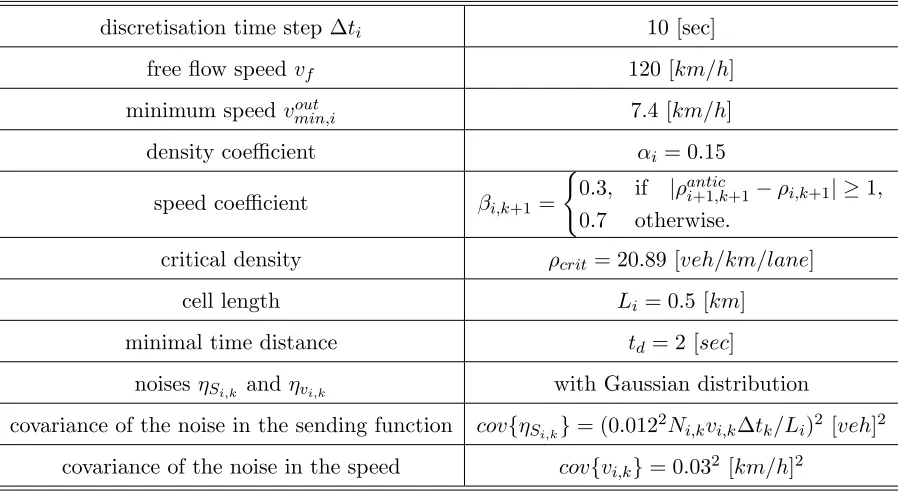
The outflow data (from cell 17) are set to be equal to the estimated ones in the previous cell 16 and this way they follow naturally the dynamics of the traffic changes. The model parameters are given in Table 1. Figure 3 presents results from the compositional model
1 1.5 2 2.5 3 3.5 4
0 0.5 1 1.5 2 2.5 3 3.5 4 Time, [h]
Number of lanes
1 1.5 2 2.5 3 3.5 4
0 1000 2000 3000 4000 5000 6000 Flow [veh/h] Time, [h] Inflow Outflow
Fig. 2. a) Number of lanes in cells 9 and 10 is changed within the interval 1.8 [h] – 3 [h]. b) Inflow (from cell 0) and outflow (cell 17). The dotted lines indicate the moments of lane change.
(1)-(9). Since usually flow-density and speed-flow diagrams are very representative for the traffic phenomenon, we show these diagrams and the evolution of the flow and speed in time. The flow is calculated on the basis of the vehiclesQi,k crossing cell boundaries.
0 50 100 150
0 2000 4000 6000
Flow, [veh/h]
Density, [veh/km]
0 2000 4000 6000
0 50 100
Flow, [veh/h]
Speed, [km/h]
1 2 3 4
0 2000 4000 6000
Flow, [veh/h]
Time, [h]
1 2 3 4
0 50 100
Speed, [km/h]
Time, [h]
1−4 5−8 9−10 11−13 14−16
[image:11.595.147.495.167.298.2]9 10
[image:11.595.133.494.392.688.2]Table 1. Simulation parameters
discretisation time step ∆ti 10 [sec]
free flow speed vf 120 [km/h]
minimum speed voutmin,i 7.4 [km/h]
density coefficient αi = 0.15
speed coefficient βi,k+1 =
(
0.3, if |ρantic
i+1,k+1−ρi,k+1| ≥1,
0.7 otherwise.
critical density ρcrit= 20.89 [veh/km/lane]
cell length Li= 0.5 [km]
minimal time distance td= 2 [sec]
noisesηSi,k andηvi,k with Gaussian distribution
covariance of the noise in the sending function cov{ηSi,k}= (0.012
2N
i,kvi,k∆tk/Li)2 [veh]2
covariance of the noise in the speed cov{vi,k}= 0.032 [km/h]2
From the results in Fig. 3 we see bell-shaped forms of the flow-density and speed-flow diagrams (the top left and right plots) which agree with the theory. Backward waves are provoked by the reduction of the number of lanes (evident also from the two bottom plots). After the first lane change (from 3 to 2) at 1.8 [h], the freeway cells are able to accept all the incoming vehicles and there is no congestion (evident from Fig. 3 bottom left), although the speed is gradually decreased (Fig. 3, bottom right). When the number of lanes ℓ drops to 1, at 2.25 [h], this provokes a congestion, and a backward wave, as seen especially from the results on the bottom of Fig. 3. After the increase of ℓto 2 at 2.75 [h], the speeds gradually increase which is reflected in an increase of the flow. Cells 11–16 behave in a different way (there is no jam) since there ℓ= 3 always and the vehicles can freely adjust their speed.
We observe reduction of the speed in cells 1-8 (bottom right plot). The speed in cell 5 is slightly increased because vehicles can move freely (the downstream density is small and there are 3 lanes). This allows the vehicles of cell 4 to increase their speed, despite the reduction in the number of lanes. The flow behavior is evident from the left bottom plot. During the first reduction of the number of lanes from 3 to 2, the flow is slightly increased because the density increases, the speed is still high. During the interval of time when the number of lanes is reduced to one the flows in all cells drop.
4.2 Model validation with real traffic data
Case study set-up
seaport, subject to frequent severe congestion during rush hours. The first on- and off-ramp along the considered stretch of road lead to a parking lot along the freeway. The data (Fig. 6)
TRAVEL DIRECTIONS
Fig. 4. Schematic representation of the segmentation of the E17 case study freeway. The labels CLOF to CLO1 indicate the locations of the traffic measurement cameras.
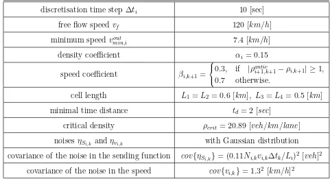
are from video cameras and are aggregated over one minute interval (to reduce the cost of the transmission from roadside sensors to the dispatching centre): average speed over all vehicles passing the sensor location during the one minute interval, and number of vehicles crossing the sensor location during the same interval. We obtained data over the whole year 2001, and selected one random day at a location where the sensors are very close together allowing proper validation. We consider the stretch between CLOF and CLOA. The cameras are positioned at the points notated by CLOF, CLOE, CLOD, CLOC, CLOB and CLOA. The measurements from CLOF are used for inflow data, respectively the measurements from CLOA are outflow boundary data for the model. Along the freeway from point CLOE to point CLOB the compositional model is computing the traffic variables. In the stretch between CLOF and CLOC there is one off-ramp and one on-ramp from a parking lot (Fig. 4). It is assumed that the number of vehicles entering the parking lot and leaving it is small so that the conservation law for the vehicles is preserved and we neglect some possibly small changes of counted vehicles. The model parameters are given in Table 2. The critical density is determined on the basis of sets of real traffic data from the same E17 freeway in Belgium. The inflow and outflow data (from CLOF and CLOA resp.) are shown in Fig. 5. The flows are quite similar over the whole time period 1−24 [h] (Fig. 5 a), the speeds differ slightly from each other in the period 1−10 [h].
5 10 15 20
0 1000 2000 3000 4000 5000 6000
Time, [h]
Flow, [veh/h]
Inflow
Outflow
5 10 15 20
0 20 40 60 80 100 120
Time, [h]
Speed, [km/h]
1
2
100 200 300 0
2000 4000 6000
Density, [veh/km]
Flow, [veh/h]
0 2000 4000 6000 0
50 100
Speed, [km/h]
Flow, [veh/h]
5 10 15 20
0 2000 4000 6000
Time, [h]
Measured vehicles, [veh]
5 10 15 200 50 100
Time, [h]
Speed, [km/h]
[image:14.595.147.479.70.348.2]CLOE CLODCLOD CLOC CLOB
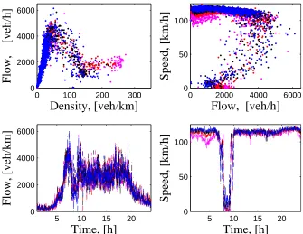
Fig. 6. Measurements from Sept. 4, 2001. Flow-density diagram (top left), flow-speed diagram (top right), evolution of the counted vehicles in time (bottom left), evolution of the speed in time (bottom right) for the period 1h – 24h. The data are obtained in four locations along the freeway (CLOE, CLOD, CLOC and CLOB from Fig. 4)
0 100 200 300
0 2000 4000 6000
Flow, [veh/h]
Density, [veh/km]
0 2000 4000 6000 0
50 100
Flow, [veh/h]
Speed, [km/h]
5 10 15 20
0 2000 4000 6000
Flow, [veh/km]
Time, [h]
5 10 15 20
0 50 100
Speed, [km/h]
Time, [h]
[image:14.595.144.479.447.706.2]The real traffic data measured at the boundaries (points CLOE, CLOD, CLOC and CLOB) are shown in Fig. 6. There are scattered and even missing data (obvious from the right bottom diagram for the speed). Nevertheless, we see a good matching of the results from the compositional model to the data (Fig. 7).
Table 2. Model parameters for the validation with real data
discretisation time step ∆ti 10 [sec]
free flow speed vf 120 [km/h]
minimum speed vout
min,i 7.4 [km/h]
density coefficient αi = 0.15
speed coefficient βi,k+1 =
0.3, if |ρantic
i+1,k+1−ρi,k+1| ≥1,
0.7 otherwise.
cell length L1 =L2 = 0.6 [km], L3 =L4 = 0.5 [km]
minimal time distance td= 2 [sec]
critical density ρcrit = 20.89 [veh/km/lane]
noises ηSi,k and ηvi,k with Gaussian distribution
covariance of the noise in the sending function cov{ηSi,k}= (0.11Ni,kvi,k∆tk/Li)
2 [veh]2
covariance of the noise in the speed cov{vi,k}= 1.32 [km/h]2
5 Conclusions
A stochastic compositional model for freeway traffic flows is proposed. It is intuitive, and generally applicable to freeways with different topologies, with any number of sensors, with regularly or irregularly received data in space and in time. The approach of modelling the traffic on freeways by the developed stochastic dynamic model with sending and receiving functions has the following features: modularity, flexibility, suitable for parallel computa-tions. Changes in the topology of the freeway network only require addition or deletion of a few components (local changes to the model). Currently we are working on an extension of the model to road networks with intersections. The inclusion in the model of weaving and merging phenomena at on- or off-ramps is another open issue for research.
The compositional model is shown to work well, both on synthetic and real traffic data sets. The model can be used for the design of recursive prediction (with the Monte Carlo filtering approach (Mihaylova & Boel, 2004)) of the state of the traffic network. These predictions in turn can serve for designing model predictive control strategies, optimizing the behavior of a network by e.g. ramp metering, or adaptive speed limits.
DWTC-CP/40 “Sustainability effects of traffic management”. We acknowledge also the financial support of the Programme on Inter-University Poles of Attraction initiated by the Belgian State, Prime Minister’s Office for Science, Technology and Culture. The authors are thankful ir. C. Carbone for the fruitful discussions on different traffic models. We also thank the Vlaams Verkeer-scentrum, Antwerp, Belgium of the Flemish Ministry of Transportation, and Mr. Frans Middleham from the Transport Research Centre of the Ministry of the Transport, the Netherlands for providing the data used in this study.
A Appendix. Algorithmic implementation of the compositional model
1.Forward wave: fori= 1,2, . . . , nm
1.1. calculate the sending function values
Si,k =max(Ni,k
vi,k.∆ti,k
Li
+ηSi,k, Ni,k
vout
min,i.∆ti,k
Li
) (A.1)
1.2. set the number of vehicles crossing the cell borders to be equal toSi,k:
Qi,k =Si,k. (A.2)
2.Backward wave: fori=nm, nm−1. . . ,1
2.1. calculate the receiving function values
Ri,k =Nimax+1,k+Qi+1,k−Ni+1,k, (A.3)
where
Nimax+1,k = (Li+1ℓi+1,k)/(Aℓ+vi+1,ktd). (A.4)
- In order to prevent possible numerical instabilities that might happen when abrupt changes occur (e.g. reduction in the number of lanes can provoke jams) the following condition is imposed:
if Ri,k <0, Ri,k =Qi+1,k.
2.2. compareSi,k and Ri,k
if Si,k < Ri,k, Qi,k =Si,k,
else Qi,k =Ri,k, vi,k =Qi,kLi/(Ni,k∆tk),
(A.5)
3. Number of vehicles inside cells, for i= 1,2, . . . , nm
Ni,k+1=Ni,k+Qi−1,k−Qi,k, (A.6)
4. Update the density, fori= 1,2, . . . , nm
ρi,k+1 =Ni,k+1/(Liℓi,k+1), (A.7)
5. Update of the speed, fori= 1,2, . . . , nm
vintermi,k+1 =
(
[vi−1,kQi−1,k+vi,k(Ni,k−Qi,k)]/Ni,k+1, forNi,k+16= 0,
vf, otherwise,
(A.9)
vinterm
i,k+1 =max(vi,kinterm+1 , vmin,iout ),
vi,k+1=βi,k+1vi,kinterm+1 + (1−βi,k+1)ve(ρantici,k+1) +ηvi,k+1, (A.10)
βi,k+1 =
(
βI, if |ρantic
i+1,k+1−ρantici,k+1| ≥ρthreshold,
βII otherwise, (A.11)
where βI < βII and ve(ρantic
i,k+1) is calculated according to (9). The second part of equation (A.9)
reflects the fact that the drivers tend to reach their free-flow speed when a cell is empty.
References
Bellemans, T. (2003). Traffic control on motorways. Ph.D. thesis, Katholieke Universiteit Leuven, Belgium.
Boel, R., & Mihaylova, L. (2004). Modelling freeway networks by hybrid stochastic models.
In Proc. of the IEEE Intelligent Vehicle Symposium (pp. 182–187). Parma, Italy.
Daganzo, C. (1994). The cell transmission model: A dynamic representation of highway traffic consistent with the hydrodynamic theory. Transportation Research B, 28B(4), 269-287.
Daganzo, C. (1995). A finite difference approximation of the kinematic wave model of traffic flow. Transportation Research B, 29B(4), 261–276.
Doucet, A., Freitas, N., & N. Gordon, E. (2001). Sequential Monte Carlo methods in
practice. New York: Springer-Verlag.
Helbing, D. (2001). Traffic and related self-driven many-particle systems.Review of Modern Physics, 73, 1067-1141.
Hilliges, M., & Weidlich, W. (1995). A phenomenological model for dynamic traffic flow in networks. Transportation Research B, 29B(6), 407–431.
Kotsialos, A., Papageorgiou, M., Diakaki, C., Pavlis, Y., & Middelham, F. (2002, December). Traffic flow modeling of large-scale motorway using the macroscopic modeling tool METANET. IEEE Trans. on Intelligent Transportation Systems, 3(4), 282-292. Mihaylova, L., & Boel, R. (2003). Hybrid stochastic framework for freeway traffic flow
modelling. In Proc. of the Intl. Symp. on Inform. and Communication Technologies
(p. 391-396). Trinity College Dublin, Ireland.
Mihaylova, L., & Boel, R. (2004). A particle filter for freeway traffic estimation. In Proc.
of the 43rd IEEE Conf. on Decision and Control (p. 2106-2111). (Atlantis, Paradise
Island, Bahamas)
Ristic, B., Arulampalam, S., & Gordon, N. (2004).Beyond the Kalman filter: Particle filters
![Fig. 2. a) Number of lanes in cells 9 and 10 is changed within the interval 1.8 [h] – 3 [h]](https://thumb-us.123doks.com/thumbv2/123dok_us/8084113.229626/11.595.133.494.392.688/fig-number-lanes-cells-changed-interval-h-h.webp)