Upper limit map of a background of gravitational waves

Upper limit map of a background of gravitational waves

B. Abbott,14R. Abbott,14R. Adhikari,14J. Agresti,14P. Ajith,2B. Allen,2,51R. Amin,18S. B. Anderson,14 W. G. Anderson,51M. Arain,39M. Araya,14H. Armandula,14M. Ashley,4S. Aston,38P. Aufmuth,36C. Aulbert,1S. Babak,1 S. Ballmer,14H. Bantilan,8B. C. Barish,14C. Barker,15D. Barker,15B. Barr,40P. Barriga,50M. A. Barton,40K. Bayer,17

K. Belczynski,24J. Betzwieser,17P. T. Beyersdorf,27B. Bhawal,14I. A. Bilenko,21G. Billingsley,14R. Biswas,51 E. Black,14K. Blackburn,14L. Blackburn,17D. Blair,50B. Bland,15J. Bogenstahl,40L. Bogue,16R. Bork,14V. Boschi,14 S. Bose,52P. R. Brady,51V. B. Braginsky,21J. E. Brau,43M. Brinkmann,2A. Brooks,37D. A. Brown,14,6A. Bullington,30 A. Bunkowski,2A. Buonanno,41O. Burmeister,2D. Busby,14R. L. Byer,30L. Cadonati,17G. Cagnoli,40J. B. Camp,22

J. Cannizzo,22K. Cannon,51C. A. Cantley,40J. Cao,17L. Cardenas,14M. M. Casey,40G. Castaldi,46C. Cepeda,14 E. Chalkey,40P. Charlton,9S. Chatterji,14S. Chelkowski,2Y. Chen,1F. Chiadini,45D. Chin,42E. Chin,50J. Chow,4

N. Christensen,8J. Clark,40P. Cochrane,2T. Cokelaer,7C. N. Colacino,38R. Coldwell,39R. Conte,45D. Cook,15 T. Corbitt,17D. Coward,50D. Coyne,14J. D. E. Creighton,51T. D. Creighton,14R. P. Croce,46D. R. M. Crooks,40 A. M. Cruise,38A. Cumming,40J. Dalrymple,31E. D’Ambrosio,14K. Danzmann,36,2G. Davies,7D. DeBra,30 J. Degallaix,50M. Degree,30T. Demma,46V. Dergachev,42S. Desai,32R. DeSalvo,14S. Dhurandhar,13M. Dı´az,33 J. Dickson,4A. Di Credico,31G. Diederichs,36A. Dietz,7E. E. Doomes,29R. W. P. Drever,5J.-C. Dumas,50R. J. Dupuis,14

J. G. Dwyer,10P. Ehrens,14E. Espinoza,14T. Etzel,14M. Evans,14T. Evans,16S. Fairhurst,7,14Y. Fan,50D. Fazi,14 M. M. Fejer,30L. S. Finn,32V. Fiumara,45N. Fotopoulos,51A. Franzen,36K. Y. Franzen,39A. Freise,38R. Frey,43

T. Fricke,44P. Fritschel,17V. V. Frolov,16M. Fyffe,16V. Galdi,46J. Garofoli,15I. Gholami,1J. A. Giaime,16,18 S. Giampanis,44K. D. Giardina,16K. Goda,17E. Goetz,42L. M. Goggin,14G. Gonza´lez,18S. Gossler,4A. Grant,40

S. Gras,50C. Gray,15M. Gray,4J. Greenhalgh,26A. M. Gretarsson,11R. Grosso,33H. Grote,2S. Grunewald,1 M. Guenther,15R. Gustafson,42B. Hage,36D. Hammer,51C. Hanna,18J. Hanson,16J. Harms,2G. Harry,17E. Harstad,43

T. Hayler,26J. Heefner,14I. S. Heng,40A. Heptonstall,40M. Heurs,2M. Hewitson,2S. Hild,36E. Hirose,31D. Hoak,16 D. Hosken,37J. Hough,40E. Howell,50D. Hoyland,38S. H. Huttner,40D. Ingram,15E. Innerhofer,17M. Ito,43Y. Itoh,51

A. Ivanov,14D. Jackrel,30B. Johnson,15W. W. Johnson,18D. I. Jones,47G. Jones,7R. Jones,40L. Ju,50P. Kalmus,10 V. Kalogera,24D. Kasprzyk,38E. Katsavounidis,17K. Kawabe,15S. Kawamura,23F. Kawazoe,23W. Kells,14 D. G. Keppel,14F. Ya. Khalili,21C. Kim,24P. King,14J. S. Kissel,18S. Klimenko,39K. Kokeyama,23V. Kondrashov,14 R. K. Kopparapu,18D. Kozak,14B. Krishnan,1P. Kwee,36P. K. Lam,4M. Landry,15B. Lantz,30A. Lazzarini,14B. Lee,50

M. Lei,14J. Leiner,52V. Leonhardt,23I. Leonor,43K. Libbrecht,14P. Lindquist,14N. A. Lockerbie,48M. Longo,45 M. Lormand,16M. Lubinski,15H. Lu¨ck,2,36B. Machenschalk,1M. MacInnis,17M. Mageswaran,14K. Mailand,14 M. Malec,36V. Mandic,14S. Marano,45S. Ma´rka,10J. Markowitz,17E. Maros,14I. Martin,40J. N. Marx,14K. Mason,17

L. Matone,10V. Matta,45N. Mavalvala,17R. McCarthy,15D. E. McClelland,4S. C. McGuire,29M. McHugh,20 K. McKenzie,4J. W. C. McNabb,32S. McWilliams,22T. Meier,36A. Melissinos,44G. Mendell,15R. A. Mercer,39

S. Meshkov,14E. Messaritaki,14C. J. Messenger,40D. Meyers,14E. Mikhailov,17S. Mitra,13V. P. Mitrofanov,21 G. Mitselmakher,39R. Mittleman,17O. Miyakawa,14S. Mohanty,33G. Moreno,15K. Mossavi,2C. MowLowry,4 A. Moylan,4D. Mudge,37G. Mueller,39S. Mukherjee,33H. Mu¨ller-Ebhardt,2J. Munch,37P. Murray,40E. Myers,15

J. Myers,15G. Newton,40A. Nishizawa,23K. Numata,22B. O’Reilly,16R. O’Shaughnessy,24D. J. Ottaway,17 H. Overmier,16B. J. Owen,32Y. Pan,41M. A. Papa,1,51V. Parameshwaraiah,15P. Patel,14M. Pedraza,14S. Penn,12 V. Pierro,46I. M. Pinto,46M. Pitkin,40H. Pletsch,2M. V. Plissi,40F. Postiglione,45R. Prix,1V. Quetschke,39F. Raab,15

D. Rabeling,4H. Radkins,15R. Rahkola,43N. Rainer,2M. Rakhmanov,32K. Rawlins,17S. Ray-Majumder,51V. Re,38 H. Rehbein,2S. Reid,40D. H. Reitze,39L. Ribichini,2R. Riesen,16K. Riles,42B. Rivera,15N. A. Robertson,14,40 C. Robinson,7E. L. Robinson,38S. Roddy,16A. Rodriguez,18A. M. Rogan,52J. Rollins,10J. D. Romano,7J. Romie,16

R. Route,30S. Rowan,40A. Ru¨diger,2L. Ruet,17P. Russell,14K. Ryan,15S. Sakata,23M. Samidi,14 L. Sancho de la Jordana,35V. Sandberg,15V. Sannibale,14S. Saraf,25P. Sarin,17B. S. Sathyaprakash,7S. Sato,23 P. R. Saulson,31R. Savage,15P. Savov,6S. Schediwy,50R. Schilling,2R. Schnabel,2R. Schofield,43B. F. Schutz,1,7

P. Schwinberg,15S. M. Scott,4A. C. Searle,4B. Sears,14F. Seifert,2D. Sellers,16A. S. Sengupta,7P. Shawhan,41 D. H. Shoemaker,17A. Sibley,16J. A. Sidles,49X. Siemens,6,14D. Sigg,15S. Sinha,30A. M. Sintes,1,35B. J. J. Slagmolen,4 J. Slutsky,18J. R. Smith,2M. R. Smith,14K. Somiya,2,1K. A. Strain,40D. M. Strom,43A. Stuver,32T. Z. Summerscales,3 K.-X. Sun,30M. Sung,18P. J. Sutton,14H. Takahashi,1D. B. Tanner,39M. Tarallo,14R. Taylor,14R. Taylor,40J. Thacker,16

S. Vass,14A. Vecchio,38J. Veitch,40P. Veitch,37A. Villar,14C. Vorvick,15S. P. Vyachanin,21S. J. Waldman,14L. Wallace,14 H. Ward,40R. Ward,14K. Watts,16D. Webber,14A. Weidner,2M. Weinert,2A. Weinstein,14R. Weiss,17S. Wen,18

K. Wette,4J. T. Whelan,1D. M. Whitbeck,32S. E. Whitcomb,14B. F. Whiting,39C. Wilkinson,15P. A. Willems,14 L. Williams,39B. Willke,2,36I. Wilmut,26W. Winkler,2C. C. Wipf,17S. Wise,39A. G. Wiseman,51G. Woan,40D. Woods,51

R. Wooley,16J. Worden,15W. Wu,39I. Yakushin,16H. Yamamoto,14Z. Yan,50S. Yoshida,28N. Yunes,32M. Zanolin,17 J. Zhang,42L. Zhang,14C. Zhao,50N. Zotov,19M. Zucker,17H. zur Mu¨hlen,36and J. Zweizig14

(LIGO Scientific Collaboration)

1_{Albert-Einstein-Institut, Max-Planck-Institut fu¨r Gravitationsphysik, D-14476 Golm, Germany} 2_{Albert-Einstein-Institut, Max-Planck-Institut fu¨r Gravitationsphysik, D-30167 Hannover, Germany}

3_{Andrews University, Berrien Springs, Michigan 49104 USA} 4_{Australian National University, Canberra, 0200, Australia} 5_{California Institute of Technology, Pasadena, California 91125, USA}

6_{Caltech-CaRT, Pasadena, California 91125, USA} 7_{Cardiff University, Cardiff, CF2 3YB, United Kingdom}

8_{Carleton College, Northfield, Minnesota 55057, USA} 9_{Charles Sturt University, Wagga Wagga, NSW 2678, Australia}

10_{Columbia University, New York, New York 10027, USA} 11_{Embry-Riddle Aeronautical University, Prescott, Arizona 86301 USA}

12_{Hobart and William Smith Colleges, Geneva, New York 14456, USA} 13_{Inter-University Centre for Astronomy and Astrophysics, Pune - 411007, India}

14_{LIGO–California Institute of Technology, Pasadena, California 91125, USA} 15_{LIGO Hanford Observatory, Richland, Washington 99352, USA} 16_{LIGO Livingston Observatory, Livingston, Louisiana 70754, USA}

17_{LIGO–Massachusetts Institute of Technology, Cambridge, Massachusetts 02139, USA} 18_{Louisiana State University, Baton Rouge, Louisiana 70803, USA}

19_{Louisiana Tech University, Ruston, Louisiana 71272, USA} 20_{Loyola University, New Orleans, Louisiana 70118, USA}

21_{Moscow State University, Moscow, 119992, Russia}

22_{NASA/Goddard Space Flight Center, Greenbelt, Maryland 20771, USA} 23_{National Astronomical Observatory of Japan, Tokyo 181-8588, Japan}

24_{Northwestern University, Evanston, Illinois 60208, USA} 25_{Rochester Institute of Technology, Rochester, New York 14623, USA} 26_{Rutherford Appleton Laboratory, Chilton, Didcot, Oxon OX11 0QX United Kingdom}

27_{San Jose State University, San Jose, California 95192, USA} 28_{Southeastern Louisiana University, Hammond, Louisiana 70402, USA} 29_{Southern University and A&M College, Baton Rouge, Louisiana 70813, USA}

30_{Stanford University, Stanford, California 94305, USA} 31_{Syracuse University, Syracuse, New York 13244, USA}

32_{The Pennsylvania State University, University Park, Pennsylvania 16802, USA}

33_{The University of Texas at Brownsville and Texas Southmost College, Brownsville, Texas 78520, USA} 34_{Trinity University, San Antonio, Texas 78212, USA}

35

Universitat de les Illes Balears, E-07122 Palma de Mallorca, Spain

36_{Universita¨t Hannover, D-30167 Hannover, Germany} 37_{University of Adelaide, Adelaide, SA 5005, Australia} 38_{University of Birmingham, Birmingham, B15 2TT, United Kingdom}

39_{University of Florida, Gainesville, Florida 32611, USA} 40_{University of Glasgow, Glasgow, G12 8QQ, United Kingdom} 41_{University of Maryland, College Park, Maryland 20742 USA} 42_{University of Michigan, Ann Arbor, Michigan 48109, USA}

43_{University of Oregon, Eugene, Oregon 97403, USA} 44_{University of Rochester, Rochester, New York 14627, USA}

45_{University of Salerno, 84084 Fisciano (Salerno), Italy} 46_{University of Sannio at Benevento, I-82100 Benevento, Italy} 47_{University of Southampton, Southampton, SO17 1BJ, United Kingdom}

48_{University of Strathclyde, Glasgow, G1 1XQ, United Kingdom} 49_{University of Washington, Seattle, Washington, 98195, USA} 50_{University of Western Australia, Crawley, WA 6009, Australia}

51_{University of Wisconsin-Milwaukee, Milwaukee, Wisconsin 53201, USA} 52_{Washington State University, Pullman, Washington 99164, USA}

(Received 31 January 2007; published 29 October 2007; publisher error corrected 4 March 2008)

We searched for an anisotropic background of gravitational waves using data from the LIGO S4 science run and a method that is optimized for point sources. This is appropriate if, for example, the gravitational wave background is dominated by a small number of distinct astrophysical sources. No signal was seen. Upper limit maps were produced assuming two different power laws for the source strain power spectrum. For anf3_{power law and using the 50 Hz to 1.8 kHz band the upper limits on the source strain power} spectrum vary between1:21048 _Hz1 _{100 Hz=f}3_and1:21047 _Hz1 _{100 Hz=f}3_{, depending} on the position in the sky. Similarly, in the case of constant strain power spectrum, the upper limits vary between8:51049_Hz1_and6:11048_Hz1_{. As a side product a limit on an isotropic background} of gravitational waves was also obtained. All limits are at the 90% confidence level. Finally, as an application, we focused on the direction of Sco-X1, the brightest low-mass x-ray binary. We compare the upper limit on strain amplitude obtained by this method to expectations based on the x-ray flux from Sco-X1.

DOI:10.1103/PhysRevD.76.082003 PACS numbers: 04.80.Nn, 02.50.Ey, 04.30.Db, 07.05.Kf

I. INTRODUCTION

A stochastic background of gravitational waves can be anisotropic if, for example, the dominant source of sto-chastic gravitational waves comes from an ensemble of astrophysical sources (e.g., [1,2]), and if this ensemble is dominated by its strongest members. So far the LIGO Scientific Collaboration has analyzed the data from the first science runs for a stochastic background of gravita-tional waves [3–5], assuming that this background is iso-tropic. If astrophysical sources indeed dominate this background, one should look for anisotropies.

A method that is optimized for extreme anisotropies, namely, point sources of stochastic gravitational radiation, was presented in [6]. It is based on the cross correlation of the data streams from two spatially separated gravitational wave interferometers, and is referred to as the radiometer analysis. We have analyzed the data of the 4th LIGO science run using this method.

Section II is a short description of the radiometer analy-sis method. The peculiarities of the S4 science run are summarized in Sec. III, and we discuss the results in Sec. IV.

II. METHOD DESCRIPTION

A stochastic background of gravitational waves can be distinguished from other sources of detector noise by cross correlating two independent detectors. Thus we cross cor-relate the data streams from a pair of detectors with a cross correlation kernel Q, chosen to be optimal for a source which is specified by an assumed strain power spectrum Hf and angular power distribution P^. Specifically, with the data stream divided into intervals labeled byt, and with~s1;tfand~s2;tfrepresenting the Fourier transforms

of the strain outputs of two detectors, this cross correlation is computed in the frequency domain interval by interval as

Yt

Z1

1

dfs~_1;tfQtfs~2;tf: (1)

In contrast to the isotropic analysis the optimal filterQ_tis now sidereal time dependent. It has the general form

Qtf t

R

S2d^^_;tfP^Hjfj

P1fP2f

(2)

wheretis a normalization factor,P1andP2are the strain

noise power spectra of the two detectors.HjfjandP^ are defined by

hh

Af^hA0f0^0i AA0ff

02^_;^0

P^Hjfj

4

(3) where Hjfjis the one-sided (positive frequencies only) spectrum of strain power, summed over both polarizations. This explains the factor of 1

4 and is appropriate for the

unpolarized stochastic background we search for. h_Af^ is

the gravitational wave strain in polarizationAat frequency farriving from the direction ^. Finally, the factor^_;t in

Eq. (2) takes into account the sidereal time dependent time delay due to the detector separation and the directionality of the acceptance of the detector pair. Assuming that the source is unpolarized,^_;t is given by

^_;tf

1 2

X

A

ei2f^*xt=c_F

1;tA^F2;tA^ (4)

where *xt x *

2;tx *

1;t is the detector separation vector,

^

is the unit vector specifying the sky position, and

F_i;tA^ _eA

ab^12X^i;taX^i;tbY^i;taY^i;tb (5)

is the response of detector i to a zero frequency, unit amplitude, A or polarized gravitational wave. eA_ab^is the spin-two polarization tensor for polarization

A and X^_i;ta and Y^_i;ta are unit vectors pointing in the directions of the detector arms (see [7] for details). The sidereal time dependence enters through the rotation of the earth, affectingX^_i;ta,Y^_i;ta, and*xt.

The optimal filterQtis derived assuming that the

intrin-sic detector noise is Gaussian and stationary over the measurement time, uncorrelated between detectors, and uncorrelated with and much greater in power than the stochastic gravitational wave signal. Under these assump-tions the expected variance,2_Yt, of the cross correlation is dominated by the noise in the individual detectors, whereas the expected value of the cross correlationYtdepends on

the stochastic background power spectrum:

2_Yt hYt2i hYti2

T

4Qt; Qt (6)

hYti T

Qt;

R

S2d^_^

;tP^H

P1P2

: (7)

Here the scalar product ; is defined as A; B

R1

1AfBfP1fP2fdfandT is the duration of the

measurement.

Equation (2) defines the optimal filter Qtfor any

arbi-trary choice ofP^. To optimize the method for finite, but unresolved astrophysical sources one should use a P^ that covers only a localized patch in the sky. But the diffraction limit of two detectors separated by d

3000 kmis given by

c

2fd

50 Hz

f : (8)

The relevant frequency depends on the assumed source power spectrumHfas well as on the noise power spectra P1 and P2, but for a typical frequency f of 300 Hz is

about 10. Thus astrophysical sources will not be spatially resolved and we can choose to optimize the method for true point sources, i.e.,P^ 2^_;^0

, which also allows for a more efficient implementation (see [6]).

We defined the strain power spectrum Hf of a point source as one-sided (positive frequencies only) and in-cluded the power in both polarizations. Thus Hf is related to the gravitational wave energy fluxFGW through

F_GWZfmax

fmin

Ffdfc 3

4G

Zfmax

fmin

Hff2_{df; (9)}

with Ff the gravitational wave energy flux per unit frequency, c the light speed, and G Newton’s constant. We look for strain power spectra Hf in the form of a power law with exponent . The amplitude at the pivot point of 100 Hz is described byH, i.e.,

Hf H

_f

100 Hz

: (10)

With this definition we can choose the normalization of the optimal filterQtsuch that Eq. (7) reduces to

hY_ti H: (11)

The data set from a given interferometer pair is divided into equal-length intervals, and the cross correlationY_tand theoretical _Yt are calculated for each interval, yielding a setfYt; Ytgof such values for each sky direction^, witht

labeling the intervals. The optimal filterQtis kept constant

and equal to its midinterval value for the whole interval. The remaining error due to this discretization is of second order in (Tseg=1 day) and is given by

YerrTseg=Y

T2 seg

24

R1

1@2^0=@t2^0H2P₁1P₂1df

R1

1j^0j2H2P1 1 P 1 2 df O _2fd c T_seg 1 day 2 (12)

withfthe typical frequency anddthe detector separation. At the same time the interval length can be chosen such that the detector noise is relatively stationary over one interval. We use an interval length of 60 sec, which guar-antees that the relative errorYerrTseg=Y is less than 1%.

The cross correlation values are combined to produce a final cross correlation estimator, Yopt, that maximizes the

signal-to-noise ratio, and has variance2 opt:

Yopt X

t

2

Yt Yt=

2

opt; opt2 X

t

2

Yt : (13)

In practice the intervals are overlapping by 50% to avoid the effective loss of half the data due to the required windowing (Hanning). Thus Eq. (13) was modified slightly to take the correlation of neighboring intervals into account.

The data was downsampled to 4096 Hz and high-pass filtered with a sixth order Butterworth filter with a cutoff frequency at 40 Hz. Frequencies between 50 and 1800 Hz were used for the analysis and the frequency bin width was 0.25 Hz. Frequency bins around multiples of 60 Hz up to the tenth harmonic were removed, along with bins near a set of nearly monochromatic injected signals used to simu-late pulsars. These artificial pulsars proved useful in a separate end-to-end check of this analysis pipeline, which successfully recovered the sky locations, frequencies, and strengths of three such pulsars listed in TableI. The result-ing map for one of these pulsars is shown in Fig.1.

III. LIGO S4 SCIENCE RUN

The LIGO S4 science run consisted of one month of coincident data taking with all three LIGO interferometers (22 February, 2005 noon to 23 March, 2005 midnight CST). During that time all three interferometers where roughly a factor of 2 in amplitude away from design sensitivity over almost the whole frequency band. Also, the Livingston interferometer was equipped with a hydrau-lic external preisolation (HEPI) system, allowing it to stay locked during daytime. This made S4 the first LIGO science run with all-day coverage at both sites. A more detailed description of the LIGO interferometers is given in [8].

Since the radiometer analysis requires two spatially separated sites we used only data from the two 4 km interferometers (H1 in Hanford and L1 in Livingston). For these two interferometers about 20 days of coincident data was collected, corresponding to a duty factor of 69%.

The large spatial separation also reduces environmental correlations between the two sites. Nevertheless we still found a comb of 1 Hz harmonics that was coherent be-tween H1 and L1. This correlation was found to be at least in part due to an exactly 1-sec periodic signal in both interferometers (Fig. 2), which was caused by cross talk from the GPS_RAMP signal. The GPS_RAMP signal consists of a sawtooth signal that starts at every full second, lasts for 1 msec, and is synchronized with the GPS re-ceivers (see Fig. 2). This ramp was used as an off-line monitor of the analog-to-digital converter (ADC) card timing and thus was connected to the same ADC card that was used for the gravitational wave channel, which resulted in a nonzero cross talk to the gravitational wave channel.

To reduce the contamination from this signal a transient template was subtracted in the time domain. This has the advantage that effectively only a very narrow band (1=run time1106 _{Hz) is removed around each}

1 Hz harmonic, while the rest of the analysis is unaffected. The waveform for subtraction from the raw (uncalibrated) data was recovered by averaging the data from the whole run in order to produce a typical second. Additionally, since this typical second only showed significant features in the first 80 msec, the transient subtraction template was set to zero (with a smooth transition) after 120 msec. This subtraction was done for only H1 since adding repetitive data to both detectors can introduce an artificial correla-tion. It eliminated the observed correlacorrela-tion. However, due to an automatically adjusted gain between the ADC card and the gravitational wave channel, the amplitude of the transient waveform is affected by a residual systematic error. Its effect on the cross correlation result was estimated by comparing maps with the subtraction done on either H1 or L1. The systematic error is mostly concentrated around the North and South Poles, with a maximum of about 50% of the statistical error at the South Pole. In the declination

FIG. 1 (color). Injected pulsar No. 3: The analysis was run using the 108.625 Hz –109.125 Hz frequency band. The artificial signal of pulsar No. 3 at 108.86 Hz stands out with a signal-to-noise ratio of 9.2. The circle marks the position of the simulated pulsar.

TABLE I. Injected pulsars: The table shows the level at which the three strongest injected pulsars were recovered.Hdfdenotes the rms strain power over the 0.5 Hz band that was used. The reported values for the injectedHdfinclude corrections that account for the difference between the polarized pulsar injection and an unpolarized source that is expected by the analysis. The one sigma uncertainty in the recoveredHdfis given in row two (Noise level), and the ratio between recoveredHdfand noise level is given in row five (SNR). The significant underestimate of pulsar No. 4 is due to a known bias of the analysis method in the case of a signal strong enough to affect the power spectrum estimation.

Injected pulsars

Quantity Pulsar No. 3 Pulsar No. 4 Pulsar No. 8

Frequency during S4 run 108.86 Hz 1402.20 Hz 193.94 Hz

Noise level () 1:891047 _6:041046 _1:731047

InjectedHdf(corrected for polarization) 1:741046 4:281044 1:541046

RecoveredHdfon source 1:741046 _4:051044 _1:791046

Signal-to-noise ratio (SNR) 9.2 67.1 10.3

Injected position 11 h 53 m 29.4 s 18 h 39 m 57.0 s 23 h 25 m 33.5 s

3326011:800 1227059:800 332506:700

Recovered position (max SNR) 12 h 12 m 18 h 40 m 23 h 16 m

37 13 32

range of75 to 75 the error is less than 10% of the statistical error. For upper limit calculations this systematic error is added in quadrature to the statistical error. After the S4 run the GPS_RAMP signal was replaced with a two-tone signal at 900 and 901 Hz. The beat between the two is now used to monitor the timing.

One postprocessing cut was required to deal with detec-tor nonstationarity. To avoid a bias in the cross correlation statistics the interval before and the interval after the one being analyzed are used for the power spectral density (PSD) estimate [9]. Therefore the analysis becomes vul-nerable to large, short transients that happen in one instru-ment in the middle interval — such transients cause a significant underestimate of the PSD and thus of the theo-retical standard deviation for this interval. This leads to a contamination of the final estimate.

To eliminate this problem the standard deviation is estimated for both the middle interval and the two adjacent intervals. The two estimates are then required to agree within 20%:

1 1:2 <

_middle adjacent

<1:2: (14)

The analysis is fairly insensitive to the threshold —the only significant contamination comes from very large outliers that are cut by any reasonable threshold [10]. The chosen threshold of 20% eliminates less than 6% of the data.

IV. RESULTS FROM THE S4 RUN

A. Broadband results

In this analysis we searched for an Hf following a power law with two different exponents.

(i) 3:Hf H3100 Hz=f3.

This emphasizes low frequencies and is useful when interpreting the result in a cosmological framework, since it corresponds to a scale-invariant primordial

perturbation spectrum, i.e., the GW energy per loga-rithmic frequency interval is constant.

(ii) 0:Hf H₀ (constant strain power). This emphasizes the frequencies for which the in-terferometer strain sensitivity is highest.

The results are reported as point estimateY^ and

corre-sponding standard deviation ^ for each pixel ^. The

point estimateY^ must be interpreted as best fit amplitude

Hfor the pixel^ [Eq. (11)].

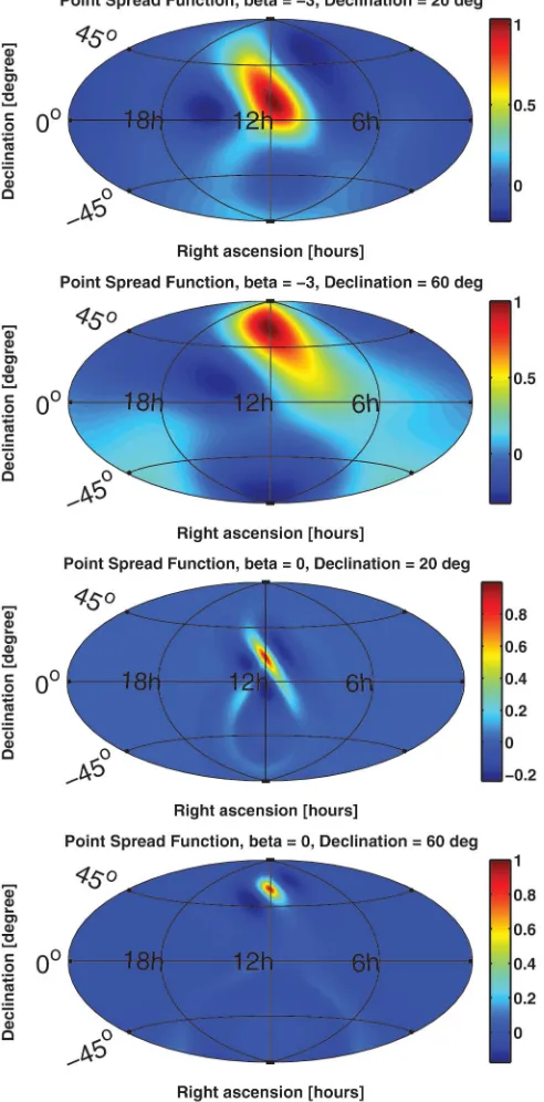
Also we should note that the resulting maps have an intrinsic spatial correlation, which is described by the point spread function

A^;^0 hY^Y^0i

hY^0Y_^ 0i

: (15)

It describes the spatial correlation in the following sense: if eitherY^0 Y due to random fluctuations, or if there is a

true source of strengthYat^0, then the expectation value at^ ishY^i A^;^

0

_{Y. The shape ofA}^_;^0

depends strongly on the declination. Figure 3 showsA^;^0 for different source declinations and both the 3 and 0case, assuming continuous day coverage.

1. Scale-invariant case, 3

A histogram of the SNRY=(SNR, signal-to-noise ratio) is plotted in Fig. 4. The data points were weighted with the corresponding sky area in square degrees. Because neighboring points are correlated, the effective number of independent points N_eff is reduced. Therefore the histo-gram can exhibit statistical fluctuations that are signifi-cantly larger than those naively expected from simply counting the number of pixels in the map, while still being consistent with (correlated) Gaussian noise. Indeed the histogram in Fig.4features a slight bump aroundSNR

2, but is still consistent withNeff 100— the dash-dotted

lines indicate the one sigma band around the ideal

0 50 100 150

−1 0 1 2

msec

uVolt Pentek

H1:DARM_ERR (1437280 averages)

0 2 4 6 8 10 12 14

−1 0 1 2

msec

uVolt Pentek

H1:DARM_ERR (1437280 averages)

0 50 100 150

−4 −2 0 2 4

msec

uVolt Pentek

L1:DARM_ERR (1447904 averages)

0 2 4 6 8 10 12 14

−4 −2 0 2 4

msec

uVolt Pentek

L1:DARM_ERR (1447904 averages)

FIG. 2. Periodic timing transient in the gravitational wave channel (DARM_ERR), calibrated inVat the ADC (Pentek card) for H1 (left two graphs) and L1 (right two graphs) shown with a span of 200 and 14 msec in black. Thexaxis is the offset from a full GPS second. About1:4106 _{secof DARM_ERR data was averaged to get this trace. Also shown in gray is the GPS_RAMP signal that} was used as a timing monitor. It was identified as a cause of the periodic timing transient in DARM_ERR. The H1 trace shows an additional feature at 6 msec.

Gaussian for Neff 100. Additionally the SNR

distribu-tion also passes a Kolmogorov-Smirnov test forNeff 100

at the 90% significance level.

The number of independent pointsN_eff, which in effect describes the diffraction limit of the LIGO detector pair,

was estimated by 2 heuristic methods.

(i) Spherical harmonics decomposition of the SNR map. The resulting power versus l graph shows structure up to roughly l9 and falls off steeply above that —the l9 point corresponds to one twentieth of the maximal power. The effective num-ber of independent points then isNeff l12

100.

(ii) FWHM area of a strong injected source, which is latitude dependent but of the order of 800 square degrees. To fill the sky we need aboutNeff50of

those patches. We used the higher estimate Neff

100for this discussion.

Figure 4 suggests that the data are consistent with no signal. Thus we calculated a Bayesian 90% upper limit for each sky direction. The prior was assumed to be flat between zero and an upper cutoff set to 51045 _Hz1

at 100 Hz, the approximate limit that can be set from just operating a single LIGO interferometer at the S4 sensitiv-ity. Note, however, that this cutoff is so high that the upper limit is completely insensitive to it. Additionally we margi-nalized over the calibration uncertainty of 8% for H1 and 5% for L1 using a Gaussian probability distribution. The resulting upper limit map is shown in Fig. 5. The upper limits on the strain power spectrum Hf vary between

1:21048 Hz1 100 Hz=f3 _{and 1:210}47 _Hz1 100 Hz=f3_{, depending on the position in the sky. These}

strain limits correspond to limits on the gravitational wave energy flux per unit frequency Ff varying between3:8106 _{erg cm}2_Hz1_{100 Hz=fand3:8}

105 _{erg cm}2_Hz1 _{100 Hz=f.}

FIG. 3 (color). Point spread functionA^_;^0

of the radiome-ter for 3 (top two figures) and for 0 (bottom two figures). Plotted is the relative expected signal strength assuming a source at right ascension 12 h and declinations 20 and 60. Uniform day coverage was assumed, so the resulting shapes are independent of right ascension. An Aitoff projection was used to plot the whole sky.

−50 0 5

1000 2000 3000 4000 5000 6000

SNR

sky area (deg

2 )

S4, beta=−3 Histogram of SNR (40 bins)

Data

Ideal Gaussian (sigma=1 mean=0)

Max Likelihood: sigma=0.91836 mean=0.11816 1−sigma error for 100 indep. points

FIG. 4. S4 Result: Histogram of the signal-to-noise ratio (SNR) for 3. The gray curve is a maximum likelihood Gaussian fit to the data. The black solid line is an ideal Gaussian, the two dash-dotted black lines indicate the expected one sigma variations around this ideal Gaussian for 100 independent points (Neff 100).

2. Constant strain power,0

Similarly, Fig.6shows a histogram of theSNRY= for the constant strain power case. Structure in the spheri-cal harmonics power spectrum goes up tol19, thusNeff

was estimated to beNeff l12 400. Alternatively

the FWHM area of a strong injection covers about1002

which also leads to N_eff 400. The dash-dotted lines in the histogram (Fig. 6) correspond to the expected one sigma deviations from the ideal Gaussian forN_eff 400. The histogram is thus consistent with (correlated) Gaussian noise, indicating that there is no signal present. The SNR distribution also passes a Kolmogorov-Smirnov test for Neff 400at the 90% significance level.

Again we calculated a Bayesian 90% upper limit for each sky direction, including the marginalization over the

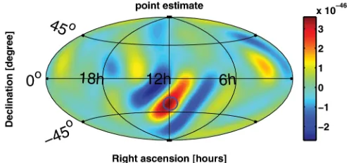
calibration uncertainty. The prior was again assumed to be flat between 0 and an upper cutoff of 51045 Hz1 at 100 Hz. The resulting upper limit map is shown in Fig.7. The upper limits on the strain power spectrum Hfvary between 8:51049 _Hz1 _{and 6:110}48 _Hz1

de-pending on the position in the sky. This corresponds to limits on the gravitational wave energy flux per unit fre-quency Ff varying between 2:7106 _{erg cm}2_Hz1 f=100 Hz2_and1:9105 _{erg cm}2_Hz1_{f=100 Hz}2_.

3. Interpretation

The maps presented in Figs.5and7represent the first directional upper limits on a stochastic gravitational wave background ever obtained. They are consistent with no gravitational wave background being present. This search is optimized for well localized, broadband sources of gravitational waves. As such it is best suited for unex-pected, poorly modeled sources.

In order to compare the result to what could be expected from known sources we also search for the gravitational radiation from low-mass x-ray binaries (LMXBs). They are accretion-driven spinning neutron stars, i.e., narrow band sources and thus not ideal for this broadband search. However they have the advantage that we can predict the gravitational wave energy flux based on the known x-ray flux. If gravitational radiation provides the torque balance for LMXBs, then there is a simple relation between the gravitational wave energy fluxF_GWand x-ray fluxF_X[11]:

F_GW fspin

fKepler

F_X: (16)

Here fKepler is final orbital frequency of the accreting

matter, about 2 kHz for a neutron star, and fspin is the

spin frequency.

As an example we estimate the gravitational wave en-ergy flux of all LMXBs within the Virgo galaxy cluster. Their integrated x-ray flux is about 109 erg=sec=cm2

(3000 galaxies at 15 Mpc, 1040 erg=sec=galaxy from

FIG. 5 (color). S4 Result: Map of the 90% confidence level Bayesian upper limit onHfor 3. The upper limit varies between1:21048 _Hz1_{100 Hz=f}3_and1:21047_Hz1

100 Hz=f3_{, depending on the position in the sky. All} fluctua-tions are consistent with the expected noise.

−50 0 5

1000 2000 3000 4000 5000

SNR

sky area (deg

2)

S4, beta=0 Histogram of SNR (40 bins)

Data

Ideal Gaussian (sigma=1 mean=0)

Max Likelihood: sigma=0.99738 mean=−0.025485 1−sigma error for 400 indep. points

FIG. 6. S4 Result: Histogram of the SNR for0. The gray curve is a maximum likelihood Gaussian fit to the data. The black solid line is an ideal Gaussian, the two dash-dotted black lines indicate the expected one sigma variations around this ideal Gaussian for 400 independent points (Neff400).

FIG. 7 (color). S4 Result: Map of the 90% confidence level Bayesian upper limit on Hfor0. The upper limit varies between8:51049_Hz1_and6:11048_Hz1_{depending on} the position in the sky.

LMXBs). For simplicity we assume that the ensemble produces a flat strain power spectrum Hf over a band-widthf. Then the strength of this strain power spectrum is about

Hf 2G c3

1

f_Keplerf_centerfFX

1055 _Hz1

_{100 Hz}

fcenter

_{100 Hz}

f

: (17)

Herefcenteris the typical frequency of thefwide band of

interest. This is quite a bit weaker than the upper limit set in this paper, which is mostly due to the fact that the intrinsically narrow band sources are diluted over a broad frequency band.

B. Limits on isotropic background

It is possible to recover the estimate for an isotropic background as an integral over the map (see [6]). The corresponding theoretical standard deviation would require a double integral with essentially the point spread function as integrand. In practice it is simpler to calculate this theoretical standard deviation directly by using the overlap reduction function for an isotropic background (see [7]). From that the 90% Bayesian upper limit can be calculated, which is additionally marginalized over the calibration uncertainty.

Limits on an isotropic background of gravitational waves are traditionally quoted as either the strain power spectrumSGWfseen by an interferometer, or asGWf,

the GW energy density per unit logarithmic frequency, divided by the critical energy density c to close the

Universe. They are related toHfby

_GWf 10

2

3H₀2 f

3_S Gwf

83

3H2₀f

3_{Hf: (18)}

HereH₀72 km sec1_Mpc1 _{is the Hubble constant}

to-day. We again assume a power law for these quantities,

S_GWf S_GW;

_f

100 Hz

_GWf _GW;

_f

100 Hz

3

;

(19)

and set a limit on their amplitude. For the scale-invariant case 3we can set a 90% upper limit of1:20104

on GW;3. Table II summarizes the results for both

choices of.

Interpretation

In [3] we published an upper limit ofGW<6:5105

on an isotropic gravitational wave background using S4 data. That analysis is mathematically identical to inferring the point estimate as an integral over the map [6], but the mitigation of the timing transient and the data quality cuts were sufficiently different to affect the point estimate. While both results are consistent within the error bar of the measurement, this difference results in a slightly higher upper limit. Both results are significantly better than the previously published LIGO S3 result.

C. Narrow band results targeted on Sco-X1

As an application we again focus on LMXBs. The gravitational wave flux from all LMXBs is expected to be dominated by the brightest one, Sco-X1, simply because Sco-X1 dominates the x-ray flux from all LMXBs, and x-ray flux FX is related to the gravitational

wave energy flux FGW through Eq. (16). Unfortunately

the spin frequency of Sco-X1 is not known. We thus want to set an upper limit for each frequency bin on the rms strain coming from the direction of Sco-X1

(right ascension: 16 h 19 m 55.0850 s;

declination:1538024:900).

The binary orbital velocity of Sco-X1 is about 40

5 km=sec (see [12]). This induces a maximal frequency shift off_GW 2:7104_f

GW. We chose a bin width

of df0:25 Hz, which is broader than maximal fre-quency shift f_GW for all frequencies below 926 Hz and is the same bin width that was used for the broadband

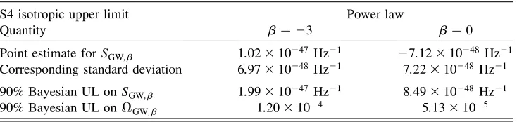
TABLE II. S4 isotropic result for theGWf const, ( 3) and the SGWf const, (0) case. The first two lines show the point estimate and standard deviation that are used to calculate the 90% Bayesian upper limits. The upper limits (UL) are also marginalized over the calibration uncertainty. These results agree with the ones published in [3] within the error bar of the measurement.

S4 isotropic upper limit Power law

Quantity 3 0

Point estimate forSGW; 1:021047 Hz1 7:121048Hz1 Corresponding standard deviation 6:971048 _Hz1 _7:221048_Hz1 90% Bayesian UL onSGW; 1:991047 Hz1 8:491048Hz1

90% Bayesian UL onGW; 1:20104 5:13105

analysis. Above 926 Hz the signal is guaranteed to spread over multiple bins.

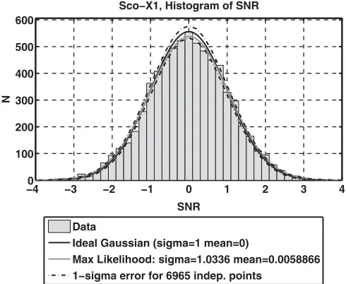
To avoid contamination from the hardware-injected pul-sars, the 2 frequency bins closest to a pulsar frequency were excluded. Multiples of 60 Hz were also excluded. The lowest frequency bin was at 50 Hz, the highest one at 1799.75 Hz. Figure8shows a histogram of the remaining 6965 0.25 Hz wide frequency bins. It is consistent with a Gaussian distribution (Kolmogorov-Smirnov test with N6965at the 90% significance level).

A 90% Bayesian upper limit for each frequency bin was calculated based on the point estimate and standard devia-tion, including a marginalization over the calibration un-certainty. Figure9is a plot of this 90% limit (black trace). Above about 200 Hz (shot noise regime above the cavity pole) the typical upper limit rises linearly with frequency and is given by

hrms90%3:41024

_f

200 Hz

; f*200 Hz: (20)

The standard deviation is also shown in gray.

Interpretation

In principle, the radiometer analysis is not an optimal method to search for a presumably periodic source like Sco-X1. Nevertheless it can set a competitive upper limit with a minimal set of assumptions on the source and significantly less computational resources. Indeed LIGO published a 95% upper limit on gravitational radiation amplitude from Sco-X1 of 1:71022 _{to 1:310}21

across the 464 – 484 Hz and 604 – 624 Hz frequency bands [13], using data from S2, which had a noise amplitude about 4.5 times higher around 500 Hz in each instrument. The analysis was computationally limited to using 6 h of data and two 20 Hz frequency bands. However the strain amplitude sensitivity of the radiometer analysis scales as T1=4 _{[6], while a coherent method scales asT}1=2_.

The upper limit [Eq. (20)] can directly be compared to the expected strain based on the x-ray flux:

hrms90%

hLX

rms

100

_f

200 Hz

₃₌₂

; f*200 Hz: (21)

Here fis the gravitational wave frequency, i.e., twice the (unknown) spin frequency of Sco-X1. This is close enough that, if the model described in [11], and thus Eq. (16) are indeed correct, Sco-X1 ought to be detectable with this method and the next generation of gravitational wave detectors operated in a narrow band configuration (AdvLIGO [14]). For a discussion of the expected signal from Sco-X1 see also [13].

V. CONCLUSION

We produced the first upper limit maps for a stochastic gravitational wave background by applying a method that is described in [6] to the data from the LIGO S4 science run. No signal was seen and upper limits were set for two different choices for the strain power spectrum Hf. In the case ofHf /f3_{the upper limits for a point source}

vary between 1:21048 _Hz1 _{100 Hz=f}3 _{and 1:2}

1047 _Hz1_{100 Hz=f}3_{, depending on the position in the}

sky (see Fig.5). Similarly, in the case of constantHfthe upper limits vary between 8:51049 Hz1 and 6:1

1048 Hz1 (see Fig. 7). As a side product limits on an

102 103

10−24

10−23

10−22

Hz

strain

Sco−X1, ra= 16.332 h , decl= −15.6402 deg

90% Bayesian limit Standard deviation

FIG. 9. S4 Result for Sco-X1: The 90% confidence Bayesian upper limit as a function of frequency — marginalized over the calibration uncertainty. The standard deviation (one sigma error bar) is shown in gray.

−40 −3 −2 −1 0 1 2 3 4

100 200 300 400 500 600

SNR

N

Sco−X1, Histogram of SNR

Data

Ideal Gaussian (sigma=1 mean=0)

Max Likelihood: sigma=1.0336 mean=0.0058866 1−sigma error for 6965 indep. points

FIG. 8. S4 Result for Sco-X1: Histogram of the signal-to-noise ratio calculated for each 0.25 Hz wide frequency bin. There are no outliers.

isotropic background of gravitational waves were also obtained, see TableII.

In an additional application, narrow band upper limits were set on the gravitational radiation coming from the brightest low-mass x-ray binary, Sco-X1 (see Fig.9). In the shot noise limited frequency band (above about 200 Hz) the limits on the strain in each 0.25 Hz wide frequency bin follow roughly

hrms90%3:41024

_f

200 Hz

; f*200 Hz; (22)

wherefis the gravitational wave frequency (twice the spin frequency).

ACKNOWLEDGMENTS

The work described in this paper was part of the doctoral thesis of S. W. Ballmer at the Massachusetts Institute of Technology [10]. Furthermore the authors gratefully ac-knowledge the support of the U.S. National Science

Foundation for the construction and operation of the LIGO Laboratory and the Particle Physics and Astronomy Research Council of the United Kingdom, the Max-Planck-Society, and the State of Niedersachsen, Germany, for support of the construction and operation of the GEO600 detector. The authors also gratefully ac-knowledge the support of the research by these agencies and by the Australian Research Council, the Natural Sciences and Engineering Research Council of Canada, the Council of Scientific and Industrial Research of India, the Department of Science and Technology of India, the Spanish Ministerio de Educacion y Ciencia, The National Aeronautics and Space Administration, the John Simon Guggenheim Foundation, the Alexander von Humboldt Foundation, the Leverhulme Trust, the David and Lucile Packard Foundation, the Research Corporation, and the Alfred P. Sloan Foundation. This paper has been assigned the LIGO document number LIGO-P060029-00-Z.

[1] L. Bildsten, Astrophys. J.501, L89 (1998)

[2] T. Regimbau and J. A. de Freitas Pacheco Astron. Astrophys.376, 381 (2001).

[3] B. Abbottet al., Astrophys. J.659, 918 (2007). [4] B. Abbottet al., Phys. Rev. Lett.95, 221101 (2005). [5] B. Abbottet al., Phys. Rev. D69, 122004 (2004). [6] S. W. Ballmer, Classical Quantum Gravity 23, S179

(2006).

[7] B. Allen and J. D. Romano, Phys. Rev. D 59, 102001 (1999).

[8] B. Abbott et al., Nucl. Instrum. Methods Phys. Res.,

Sect. A517, 154 (2004).

[9] A. Lazzarini and J. Romano, http://www.ligo.caltech.edu/ docs/T/T040089-00.pdf.

[10] S. W. Ballmer, Ph.D. thesis, Massachusetts Institute of Technology (MIT), 2006.

[11] R. V. Wagoner, Astrophys. J.278, 345 (1984).

[12] D. Steeghs and J. Cesares, Astrophys. J.568, 273 (2002). [13] B. Abbottet al., arXiv:gr-qc/0605028 [Phys. Rev. D (to be

published)].