Impact Hazard Protection Efficiency by a Small Kinetic
Impactor
J.P. Sanchez1
University of Strathclyde, Glasgow, Scotland G1 1XH, United Kingdom
C. Colombo2
University of Strathclyde, Glasgow, Scotland G1 1XH, United Kingdom
In this paper the ability of a small kinetic impactor spacecraft to mitigate an
Earth-threatening asteroid is assessed by means of a novel measure of efficiency. This measure
estimates the probability of a space system to deflect a single randomly-generated
Earth-impacting object to a safe distance from the Earth. This represents a measure of
efficiency that is not biased by the orbital parameters of a test-case object. A vast
number of virtual Earth-impacting scenarios are investigated by homogenously
distributing in orbital space a grid of 17,518 Earth impacting trajectories. The relative
frequency of each trajectory is estimated by means Opik’s theory and Bottke’s near
Earth objects model. A design of the entire mitigation mission is performed and the
largest deflected asteroid computed for each impacting trajectory. The minimum
detectable asteroid can also be estimated by an asteroid survey model. The results show
that current technology would likely suffice against discovered airburst and local
damage threats, whereas larger space systems would be necessary to reliably tackle
impact hazard from larger threats. For example, it is shown that only 1,000 kg kinetic
impactor would suffice to mitigate the impact threat of 27.1% of objects posing similar
threat than that posed by Apophis.
Nomenclature
a = semi-major axis of an orbit, km
b* = b-plane impact parameter, km
D = asteroid’s diameter, km or m
1 [email protected], Research Fellow, Advanced Space Concepts Laboratory, Department of Mechanical and Aerospace Engineering, University of Strathclyde, Glasgow
2
DElowbound = asteroid’s diameter yielding minimum energy in an energy event, km or m DEupperbound = asteroid’s diameter yielding maximum energy in an energy event, km or m
DMaxsize = maximum asteroid’s diameter that can be deflected within a twarning, km or m DMinsize = minimum asteroid’s diameter discovered within a tsurvey, km or m
dmin = minimum distance, km or AU
Eimpact = impact energy, MT
e = eccentricity of an orbit
eimpact = specific impact energy, J/kg
fI(.) = asteroid’s impact probability
G = phase slope parameter
g(.) = collision probability function
H = asteroid’s absolute magnitude
IeventD = impact event cumulative distribution
Isp = specific impulse of a propulsion system, s i = inclination of an orbit, deg
l = distance between Earth and asteroid when the latter is at its MOID-zero point, km or AU
M = mean anomaly of an orbit, deg
MAst = mass of the asteroid, kg
MOID = critical MOID for which an asteroid would impact Earth
md = mass of the spacecraft at impact, kg N(.) = cumulative number of objects
Pcol:MOID=0 = probability of collision with Earth of a MOID-zero orbit
p = semilatus rectum of an orbit, km
pv = asteroid´s albedo
R = distance between the asteroid and the Earth, AU
R = distance between the asteroid and the Sun, AU
ra = minimum distance between the Earth and the hyperbola´s asymptote, km rp = periapsis distance, km
ToF = time of flight of the transfer, s
t = time, s or d
td = deflection time or time at which impact occurs, s or d
timpact = time at which the asteroid is bound to impact the Earth, s or d
tlaunch = time at which spacecraft is launched from Earth, s or d
tsf = final time of the asteroid’s survey, s or d tsi = initial time of the asteroid’s survey, s or d V = asteroid’s apparent magnitude
Vlim = limiting visual magnitude
Ast
v = asteroid’s orbital velocity vector, km/s
v = Earth´s orbital velocity vector, km/s
vimpact = asteroid’s impact velocity, km/s
v∞ = hyperbolic excess velocity of the asteroid, km/s
/
S C
v = in-plane angle between the vS C/ and the vAst, rad or deg
β = momentum enhancement factor
γ = flight path angle, rad
/ S C
v = relative velocity of the spacecraft with respect to the asteroid, m/s or km/s
warning
t
= warning time, years
survey
t
= time-length of the survey campaign, years
r = displacement of the asteroid position at the impact point, km v = impulsive change of velocity vector, m/s or km/s
/
S C
v = out-of-plane h direction angle of vS C/ , rad or deg
ε = hyperbolic factor
k = solar phase angle, rad
= gravitational constant of the Sun, 3.9644x10 -14AU3/s2
= gravitational constant of the Earth, 3.9860x10⁵ km3/s2ρ(.) = near Earth asteroid density distribution
. = argument of the ascending node of an orbit, deg
Ωimpact = argument of the ascending node of an impacting trajectory, deg
= argument of the perigee of an orbit, degωimpact = argument of the perigee of an impacting trajectory, deg
= Earth´s angular velocity, rad/s
Subscripts
= relative to the Earth = relative to the Sun
I.
Introduction
Asteroids have long been recognized as both a threat to Earth, as well as an opportunity. As remnants of the formation of our solar system, asteroids and comets provide a precious opportunity to unveil the mysteries of the solar system formation, evolution and composition. On the other hand, Earth is periodically hit by these objects, which permanently alters the characteristics of our planet to varying degrees [1]. Asteroid impacts range from events causing mass extinctions such as the Cretacious-Terciary impact that resulted on the extinction of the dinosaurs [2], to much more modest impacts such as the air blast occurred in 1908 near the Russian Tunguska river [3]. The awareness of the impact risk has led to an intense surveying effort, which now-a-days is responsible for tracking about 9000 Near-Earth Objects (NEOs) [4].
The general recognition that Earth is regularly struck by small objects, together with the increasing number of asteroid discoveries, has also stimulated an intense debate on deflection strategies (see, for example, in the Planetary Defence Conference series3). An outcome of this is a growing catalogue of different concepts for asteroid deflection that range from very subtle changes on the optical properties of the asteroid [5] to the much more blunt use of nuclear warheads [6]. In between, other noticeable examples are; low-thrust tugboats [7], gravity-tractors [8], mass drivers [9], solar collectors [10] , ion-beam shepherds [11] and many others. Some of these deflection methods require substantial technological advancements, such as, for example, solar collectors or mass drivers, while others are considered to be at a high technological readiness level (TRL) [12]. Among the latter group, the simplest concept and, probably, highest TRL is the kinetic impactor strategy, which involves changing the asteroid’s linear momentum by impacting a spacecraft into it [13, 14].
Considerable efforts have also focused on comparing the different asteroid deflection concepts in an attempt to assess the optimal deflection strategy. In a NASA study [15], for example, the preliminary mission design of a comprehensive set of deflection alternatives was performed for a set of five NEO impacting scenarios. The system performance was described by the “effective momentum change” (i.e., ∆v required for the deflection multiplied by the NEO’s mass) and launch mass. Sanchez et al. [12] performed a multi-objective comparative
assessment of six different deflection strategies for thirteen different impact scenarios, characterized by different orbital elements, masses, and physical characteristics of the impacting objects. Also, Schaffer et al. [16] used a multi-objective comparison in order to select the best mitigation option against three notional asteroid impact threats. These, and other, deflection assessments reflect the challenge to define the optimality of a deflection strategy if nothing on the threatening object itself is known, and the necessity of using notional impact scenarios as test cases for the deflection methods.
This paper re-examines the kinetic impactor option while also considering the epistemic uncertainty of the asteroid impact threat. In a previous analysis on the kinetic impactor option, it was shown that with a small spacecraft and very simple transfer strategies, it is possible to obtain considerable deviations for most of the threatening asteroids [17]. In that work, optimal impact trajectories (direct and via a single Venus gravity-assist) to an extract of 30 Potentially Hazardous Asteroids (PHAs) taken from the JPL catalogue of asteroids were designed and analyzed. It has also been shown that, when compared with other more complex deflection alternatives, the kinetic impactor still offers a reasonable option for relatively small objects [12].
Thus, the paper aims to improve the understanding of the capability of a kinetic impactor with current space engineering technology to offer planetary protection from realistic impact threats. A simple figure of merit is used here to convey a good understanding of the capability of a deflection system to provide protection against the general impact hazard. This figure is named thereafter the Planetary Protection of the deflection system and provides a quantitative measure of the ability of the deflection system to mitigate any possible Earth-impacting object. This is achieved by estimating the probability of succeeding in deflecting to a safe Earth distance a randomly generated impact threat. A vast number of realistic impact threats are therefore required to be investigated in order to obtain a statistically meaningful sample of deflection scenarios.
Bottke et al. [18]. The asteroid’s argument of the periapsis ω defines then the Minimum Orbital Intersection Distance (MOID) with the Earth, whereas the mean anomaly M at a given Epoch defines the actual closest encounter. Opik’s formulation [19], together with Bottke’s Near-Earth Object distribution, is used to estimate
the relative impact frequency or probability of a hypothetical threatening object to have a given set of ephemerides.
The mitigation action produced by the kinetic impactor can be well modeled as an instantaneous variation of the velocity of the asteroid at the impact time. The conservation of linear momentum ensures then a linear relation between the mass of the asteroid and the asteroid’s variation of velocity. Thus, if the mass of the
impacting spacecraft and the impact velocity vector are defined, the size of the largest asteroid that can be deflected by a safe distance from the Earth can also be computed. For each single asteroid’s orbit in the set of virtual threatening objects an Earth-to-asteroid interception trajectory is optimized in order to maximize the displacement of the asteroid at the MOID following the kinetic deflection. The deflection achieved at the Earth is computed by an analytical formulation making use of proximal motion equations expressed as a function of orbital elements, which provides a good accuracy and reduces the computational effort [17].
The paper aims to understand the realistic capability to mitigate impact hazard with current space technology. For this reason, a small deflection mission is assumed; a 1,000 kg spacecraft is launched from Earth with 2.5 km/s of escape velocity v∞. In the view of recent missions to asteroids, such as NASA’s Dawn mission [20], ESA’s Rosetta mission4 or Deep Impact [21], this can be considered a perfectly plausible mission with current space technology. Moreover, it is important to consider that in a real impact threat scenario, i.e., when an asteroid is bound to hit the Earth, if a deflection attempt is arranged, higher levels of funding than those seen today for scientific missions should be expected, and thus, a 1-tonne deflection system can here be considered
small.
For the sake of completeness, two distinct cases are envisaged in this paper. On the first one, we assume that the impact threat is know, thus it has been previously detected and surveyed by an asteroid detection system. This allows us to define the level of planetary protection purely achieved by the kinetic impactor system. On the other hand, this can be put into a wider, and more realistic, context by considering that the impact threat requires to be detected by a survey system prior to any deflection attempt. While the definition of the kinetic deflection system (i.e., 1-tonne and excess velocity at launch of 2.5 km/s) poses a maximum limiting size that can be deflected, the need for the impacting threat to be detected imposes also a minimum object size that can
realistically tackle. For each of these two cases, one can then estimate the fraction of impact hazard (over all the possible impact scenarios) that a small kinetic deflection system should be able to mitigate.
The paper is organized as follow: Section II describes the methodology to create a comprehensive list of ephemeris made up with more than 17,000 impacting trajectories. Each impacting orbit is then tagged with its relative impact frequency. Section III gives an account of the method and model used to describe a complete deflection mission. This includes trajectory design through global optimization, the impact model and final deflection calculation. Moreover, a detection model, which attempts to provide a measure of the likelihood of discovery of an object on an Earth-impacting course, is described. As will be shown, the detection model is only a simple account that captures the essentials of the asteroid detection problem and allows us to define the capabilities of a notional asteroid survey. Section IV summarizes the results of the optimized deflection scenarios and the planetary protection achieved by a small kinetic impactor system. Finally, Section V concludes with a brief discussion of the results.
II.
Set of impacting orbits
A set of Earth-impacting orbits was created as comprehensive set of impact hazard scenarios to be tackled by a realistically-sized kinetic impactor. In order to provide an assessment of the capabilities of such a system for impact hazard mitigation, i.e., planetary protection, the number of deflection mission analyzed here needs to be much larger than in previous deflection studies [12, 17]. The set of impacting trajectories presented here is made up of 17,518 different ephemeris sets. All of these yield an impact at the same pre-defined epoch. The present section summarizes how the set of impacting orbits was created.
A. Earth impacting orbits
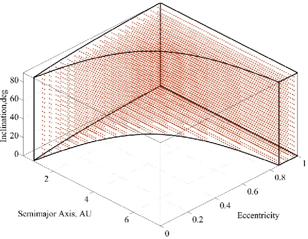
Figure 1: Homogenously distributed grid set of Earth-impacting trajectories.
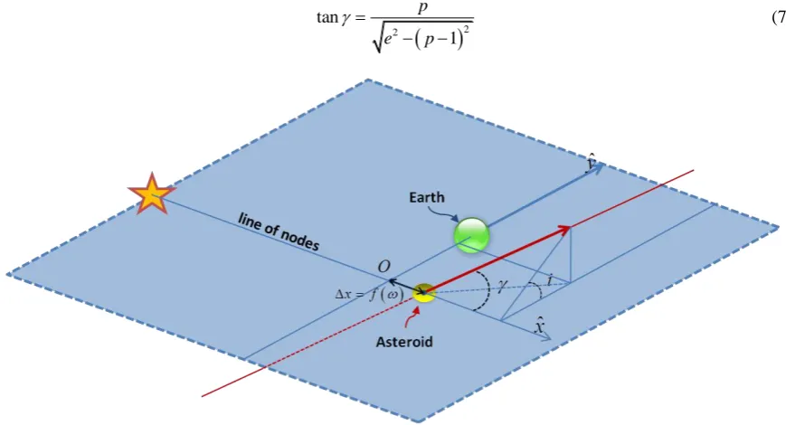
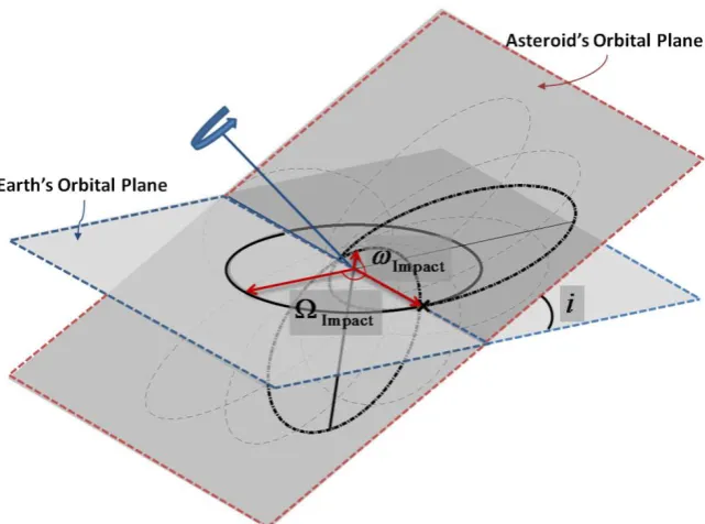
Figure 2: Orbital geometry of possible impactors for a given semi-major axis a, eccentricity e and
inclination i.
Another consequence of assuming the Earth is on a 1 AU circular orbit is that the excess velocity v∞ of any possible encounter can be defined analytically as a function of semi-major axis a, eccentricity e and inclination i
of the asteroid by means of Tisserand’s criterion:
2
3 1 2 1 cos
v a e i
a
(1)
where
is the gravitational constant of the Sun and both semi-major axis and
need to be expressed in AUunits. The final impact velocity can then be computed by accounting for the Earth’s gravity as:
2
2
impact
v v
r
(2)
where r and
represent respectively the radius and gravitational constants of the Earth. Note that thespecific impact energy, or energy-mass fraction, yielded by each impacting orbit
2
1 2
impact
impact impact
Ast E
e v
M
(3)
is also pre-defined, since vimpact is an explicit function of the impact trajectory, where MAst is the mass of the
B. Impact probability
As can be seen, for example, in Ref. [18], there are regions of space much more densely populated with near-Earth objects than others. There are, for instance, many more low inclination than high inclination objects. On the other hand, not only the NEO population density is important when considering impact frequency, but also the impact geometry of the orbit plays an important role. Thus, each of the 17,518 homogeneously distributed virtual impactors do not have the same likelihood of existing and this needs to be accounted for when considering levels of planetary protection. The relative frequency of each virtual impactor is therefore assessed individually, by means of two multiplying factors; first, the NEO orbital distribution that defines the actual asteroid probability density, and second, the collision probability of a given set of {a,e,i}, which assesses the likelihood of impact for a given object.
NEO orbital distribution
The NEO orbital distribution used here is based on an interpolation from the theoretical distribution model published in Bottke et al. [18]. The data used was very kindly provided by W. F. Bottke (personal communication, 2009). An orbital distribution of NEOs was built by propagating in time thousands of test bodies initially located at all the main source regions of asteroids (i.e., the ν6 resonance, intermediate source
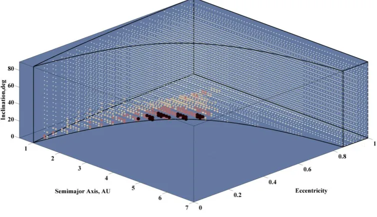
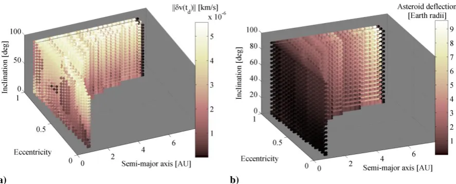
Figure 3: Theoretical Bottke et al. [18] NEO distribution. The figure shows a representation of the NEO
density function ρ(a,e,i). The 4th dimension, i.e., the density ρ at a given point (a,e,i), is represented by a
set of grid points colored and sized as a function of the value ρ. A smaller set of axes represent the
projection of the total value of ρ onto the planes a=0.5 AU, e=1 and i=0 deg. Note that the color code has
been inverted for the smaller projection figure to improve clarity.
Probability of collision of an asteroid
A necessary condition for an asteroid to impact the Earth is to have both a perihelion smaller and aphelion larger than 1 AU. This, of course, it is not sufficient, since only a very limited set of arguments of periapsis ω will actually yield a trajectory crossing Earth’s orbital path (see Figure 2). For a given epoch, that is a fixed
The MOID is referred to here as the minimum orbital distance possible between two orbits and, particularly, in the case at hand between the Earth and an asteroid. In order to compute the collision probability of an asteroid with Keplerian elements {a,e,i}, we first need to compute the maximum MOID that allows an Earth collision. For the latter, the Earth’s gravity needs to be accounted, since an asteroid close to Earth will essentially follow a hyperbolic trajectory with the Earth at its focus. A hyperbolic factor
,2
2 1
a
p p
r
r r v
(4)
accounts then for the curvature that the object’s trajectory would experience during the Earth approach. In Eq.
(4), ra is the minimum distance between the hyperbola asymptote and the Earth, rp is perigee distance of the asteroid’s hyperbolic trajectory,
is the gravitational constant of the Earth and vthe hyperbolic excessvelocity of the asteroid as given in Eq. (1). Thus, if we assume that the maximum distance for a collision to
occur is one Earth radius r, the actual maximum geometrical distance between the orbit of the Earth and the
asteroid will require to be smaller than
2
2 MOID r 1
r v
. (5)
The following sub-section will describe an analytical approximation of the MOID that allows us to easily
compute the range of argument of the periapsis ω such that the asteroid’s MOID is smaller than MOID. Two important assumptions allow us to proceed: firstly, we have already assumed a circular 1 AU orbit for the motion of the Earth, and secondly, we assume that the right ascension of the ascending node Ω and the argument of periapsis ω are uniformly distributed random variables. The ascending node Ω and the argument of periapsis
ω are generally believed to be uniformly distributed in near Earth orbit space as a consequence of the fact that
the period of the secular evolution of these two angles is expected to be much shorter than the life-span of a near Earth object. Therefore, we can assume that any value of Ω and ω is equally possible for any NEA [18]. Similarly, all values of mean anomaly M are also assumed to be equally possible.
Minimum Orbital Intersection Distance
approximated [19]. With the axis shown as in Figure 4, the motion of the Earth and the asteroid can be well described using a linear approximation of the Keplerian velocities of the two objects at the encounter. This defines two straight line trajectories, and thus, the minimum distance between these two linear trajectories can be found. The minimum distance can then be written as an explicit function of ∆x, which is defined as the distance between the centre of the coordinates described in Figure 4 and the point at which the asteroid crosses the Earth’s orbital plane. This minimum distance ∆x can alternatively be described as a linear function of the
argument of the periapsis ω. Finally, an expression such as [19]
22
MOID
1
tan sin
impact
i
(6)
yields an approximate value of the MOID distance. The absolute value |ωimpact ‒ ω| refers to the minimum absolute difference to the two values of ωimpact and the tangent of the flight path γ angle can be calculated as:
22
tan
1 p
e p
[image:13.595.87.522.347.582.2] (7)
Figure 4: Set of coordinates used to compute Eq. (6).
Probability of having a MOID lower than the collision distance
Since Eq. (5) defines the maximum MOID at which a collision would occur, by rearranging Eq. (6) it is possible to define the range of argument of periapsis for which an asteroid would have a MOID smaller than
MOID:
2 2
1
MOID tan
sini
(8)
Twice the value of Eq. (8) provides the total range of ω that yields a MOID smaller than MOID for one of the two impactors in each point of the grid, and since there are there are two different impactors, the total range shall be 4∆ω. Lastly, since the argument ω has been assumed a uniformly distributed random variable and the total range of possible arguments ω is 2π, the probability of having an argument ω such that the impact can occur is:
, ,
2 2
2
g a e i
(9)
Probability of collision
Equation (9) defines the probability of having an asteroid such that MOID is small enough for a collision to be possible, nevertheless we still require to know the probability of also having the Earth and the asteroid with a
phasing such that the collision occurs. This will now be described by defining the function g a e i
, ,
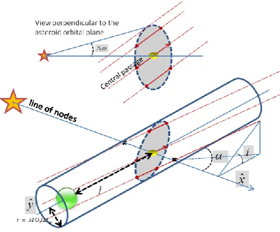
color probability of collision with Earth of an asteroid with MOID≤MOID.As is well known, the shortest distance between two linear trajectories must have a direction perpendicular to both of them, and this must also be satified by the Earth and asteroid linear trajectories as described in Figure 4. As depicted now in Figure 5, this condition defines a cylindrical region around the Earth’s linear trajectory that must be crossed by any object with a minimum orbital distance smaller than the radius of the cylinder. Since the motion of an asteroid with defined inclination i (and ascending node Ω) will always be confined within its orbital plane, an elliptical section can be defined as a result of the intersection between the cylinder of radius r and the asteroid’s orbital plane (see Figure 5). Note that since the Earth is assumed to be on a circular orbit, the right ascension of the ascending node Ω is actually irrelevant for the calculation of the impact probability. The trajectories of both objects are assumed to be straight lines. An asteroid with a MOID smaller
Figure 5: Representation of the Earth and asteroid impact geometry.
Thus, as defined in Figure 5, a necessary, but not yet sufficient, condition for an asteroid to encounter the Earth at distance smaller than r is that its trajectory must intersect the elliptical section drawn by the intersection
of a cylinder of radius r and the asteroid’s orbital plane. For the case of a cylinder of radius equal toMOID, only asteroids with arguments of periapsis within ωimpact±∆ω will have trajectories intersecting its elliptical section. Each of these trajectories (i.e., with varying ω within the range ωimpact ±∆ω) will follow parallel paths, due to the linearly approximated motion, intersecting the elliptical section for a different length, as shown in Figure 6. Aa a consequence, all trajectories would draw parallel chords in the elliptical section. Among all possible trajectories, the central passage yields the trajectory with the longest path within a distance smaller than
Figure 6: Configuration of asteroid impacting trajectories.
These intersecting trajectories can also be seen as a set of parallel chords of the elliptical section. Then, the average length of the set of parallel chords (or parallel trajectories) crossing an ellipse can be computed to be
4
times the length of the central chord/trajectory (i.e., trajectory crossing the centre of the ellipse). Similarlythen, the average probability of collision for asteroids with periapsis argument within the range ωimpact ±∆ω is assumed to be π/4 times the probability of collision of the central trajectory:
, ,
, ,
:MOID 04
col col
g a e i
P a e i (10)where Pcol:MOID=0 refers to the probability of collision with the Earth of the asteroid trajectory with MOID equal
to zero (MOID-zero object), or the central passage of the ellipse pictured in Figure 5 and Figure 6.
In order to compute Pcol:MOID=0, let us imagine the asteroid at the centre of the ellipse, or point of MOID
equal to zero, while the Earth is at a distance l from the same point (see Figure 6). The relative motion of these two bodies in radial-transversal-out-of-plane Cartesian coordinates and using AU as unit length is given by:
2 2
1 , cos , sin
e p p i p i
p
(11)
2 2 min 2 cos 1 1 p i d l v (12)If we then set the minimum distance dmin equal to the maximum MOID required for a collision, MOID, and isolate the variable l, we then obtain the range of positions for which the Earth would actually be impacted by a MOID-zero object at the MOID point:
max 2 2 MOID cos 1 v lv p i
. (13)
Finally, Pcol:MOID=0 can be easily computed by dividing the total length of possible Earth configurations allowing
it to impact the MOID-zero asteroid, i.e., 2lmax, by the total Earth path length in AU units, i.e., 2π.
Collecting the previous subsections, the collision probability of an asteroid is then given by:
max, ,
2
col
l g a e i g g
. (14)
Note that for very low inclinations or very small eccentricities, both ∆ω and lmax tend to infinity, and thus, the linear approximation ceases to be valid. To avoid this problem the upper bound of ∆ω is set to π/2, while a numerical search of lmax is performed when the linearly approximated lmax becomes larger than 0.0175 radians (i.e., 1 deg). Similarly to the linear approximation, the numerical search finds the range of the Earth’s mean anomaly ∆Mmax for which the minimum distance to a MOID-zero asteroid is equal toMOID.
Relative frequency of impactors
The set of impactors can finally be weighted with their relative frequency in order to distinguish which regions of the Keplerian element space actually yield a higher impact risk. To compute the relative frequency,
Figure 7: Set of virtual impactors plotted as dots of size and color as a function of the relative frequency
that should be expected for each impactor.
III.
Deflection scenarios and models
Once the set of Earth-impacting ephemeris has been defined, a deflection mission can be designed by modeling the transfer phase from the Earth to the asteroid interception and the following deflection phase. Then, the maximum deflection achievable for each single impacting ephemeris in the set is computed. As stated earlier, the purpose of the paper is to investigate the ability to provide planetary protection with existing space capabilities. It was therefore chosen here to analyze a kinetic impact system, which can be argued to be the simplest deflection option; other mitigation strategies may be considered in a further work.
A. Kinetic impact deflection
A kinetic impactor mission, with a 1,000 kg wet mass spacecraft and specific impulse Isp 300 s is launched from Earth with 2.5 km/s hyperbolic excess velocity at a given time tlaunch, previous to the time at which the asteroid is bound to impact Earth timpact. The Earth to asteroid transfer is modeled as direct Lambert’s arc with less than one revolution around the Sun. The kinetic impactor spacecraft intercepts and hits the asteroid
at a certain deflection time tdtlaunchToF, where ToF is the time of flight of the transfer. The impact between the spacecraft and the asteroid is considered to be perfectly inelastic, such that the variation of orbital
/
d
d S C d
Ast d
m
t t
M m
v v (15)
where the relative velocity vS C/
td of the spacecraft with respect to the asteroid at the deflection point iscomputed from the ephemerides of the asteroid at the deflection time tdand from the solution of Lambert’s arc
trajectory. The parameter β represents the momentum enhancement factor, which takes into account effects due to the ejection of mass or gasses, and was set to a conservative value of 1. The mass of the spacecraft at the impact with the asteroid md is computed from the rocket equation, subtracting the propellant mass used during
the transfer, and MAst is the mass of the asteroid.
The displacement of the asteroid position at the encounter r
timpact
following the deflection maneuver Eq. (15) is computed through an analytical formulation derived by Vasile and Colombo [17]:
timpact
timpact,td
tdr Φ v (16)
where Φtimpact,td is the transition matrix defined through the proximal motion equations and Gauss’s
planetary equations. The deflection r
timpact
is then translated into the impact parameter b* on the b-plane [19], which describes the minimum intersection distance between the deflected asteroid and the Earth, through a matrix rotation described in [17]. Furthermore, the effect of the Earth’s gravity on the deflected trajectory of the asteroid is taken into account by including the hyperbolic factor:2 *2
4 2
p
r b
v v
(17)
where v
vAstv
is the relative velocity of the asteroid with respect to the Earth as given in Eq. (1). Note that Eq. (17) can be rearranged to obtain Eq. (5) if the perigee of the hyperbolic trajectory under the Earth’sgravity is set equal to r.
Through the analytical formulation in Eq. (16) it was possible to define the optimal direction of the
deflection maneuver v
td in order to maximize the magnitude of the deflection rp for a given time-to-impactimpact d
B. Mission design
A global optimization procedure is used to select the optimal transfer conditions to deflect each virtual threatening object on the orbital elements grid by maximizing Eq. (17). Being the impact time defined, the design parameters of the mission are the launch date tlaunch and transfer time ToF, which, by defining the
Lambert’s arc trajectory, also specify the impact conditions (i.e., vS C/
td and md) in Eq. (15) and, thus, thedeflection achieved at the Earth’s encounter. A global optimization method is used that blends a stochastic search with an automatic solution space decomposition technique. This method has proven to be particularly effective when compared to common optimization methods, especially when applied to space trajectory optimization problems [23, 24]. The time of flight of the transfer trajectory can be chosen within a range
0.01 1.1
T where T indicates the greater value between the period of the asteroid and the period of theEarth’s orbit around the Sun. Setting the impact date timpact and a warning time twarning, the launch date can be
chosen within the range:
launch impact warning warning 0 0.99
t t t t ToF (18)
such that the time-to-impact timpacttd can span from twarningToF down to
twarningToF
0.01. Thewarning time twarningis then a paramount parameter of the impact scenario, since it defines the length of the time window within which both transfer and deflection require to be performed. In order to better scan the extended warning time window, two global optimizations are performed; in the first one the search domain can be divided by the optimizer into a sub-domain along the launch time direction down to a depth of branching equal to two. In this way particular regions of the warning time window can be better investigated. Afterwards a subsequent optimization procedure is done, starting with the optimal population of the first run, where the whole domain is explored without any subdivisions [23, 24].
The optimization procedure defines the optimal departure and transfer conditions to maximize the asteroid deflection at the Earth’s encounter; in particular this defines the direction of the impacting maneuver on the
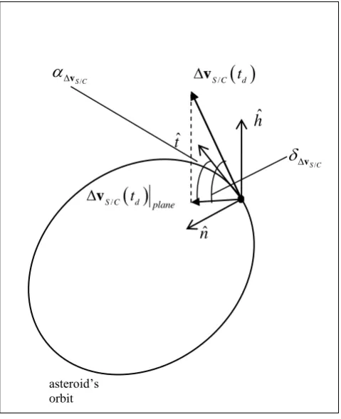
asteroid. In order to show the influence of the asteroids’ orbital elements on the deflection strategy, Figure 9 shows the direction of the deflecting maneuver relative to asteroid’s nominal orbit, specifically measured in local tangential-normal-h reference frame centered at asteroid at the point of interception by the kinetic impactor
spacecraft. We define
/
S C
v as the magnitude of the angle between the projection of vS C/
td on the orbitalby the kinetic impactor spacecraft. Analogously,
/
S C
v is here defined to be the magnitude of the angle between
/S C td
v and S C/
dplane t
v . Figure 8 shows the angles
/
S C
[image:21.595.179.419.132.427.2]
v and
vS C/ .Figure 8: Geometry of the deflection.
The angle
/
S C
v , used as color scale in Figure 9a, indicates how far the component of the deflecting action
is on the asteroid plane from the tangential direction. It can be noted that for low-inclination asteroids the relative velocity of the spacecraft with respect to the asteroid has a non-zero component along the normal direction in the asteroid orbit plane; for highly inclined asteroids, instead, the velocity of the impacting spacecraft is almost perpendicular to the asteroid nominal orbit plane, as the asteroid is intercepted very close to the ascending node. As a consequence, the relative velocity, has only some component in the out-of plane h
direction and in the tangential direction, but no component in the normal direction. Moreover it can be asserted that most of the deflection scenarios have the spacecraft breaking the asteroid (the dot symbol in Figure 9a
indicates a negative component of vS C/
td plane along the tangential direction) and in only few of the scenariosthe spacecraft is accelerating the asteroid (the cross symbol in Figure 9a indicates a positive component of
/
S C td plane
v along the tangential direction).
asteroid’s orbit orbit
ˆ
t
/ S Ct
d
v
/
S C
t
d plane
v
ˆ
n
ˆ
h
/ S C
v/
S C
Analogously, in Figure 9b each point of the grid is colored according to angle
/
S C
v which gives an
indication on how much the deflection maneuver is out of the orbital plane of the asteroid. Moreover the cross or dot symbols in Figure 9b indicate whether the h-component of the maneuver is in the –h or +h direction, respectively. These results are in agreement with the results in Vasile and Colombo [17] although the deflection trajectories are here computed on a much larger set of asteroids, with a wider range of orbital elements. Future work will show a deeper analysis of the deflection trajectories; this is not in our purpose here, hence we limited to discuss the general trend of the deflection trajectory with the asteroid’s orbital elements.
[image:22.595.78.522.262.439.2]
a) b)
Figure 9: direction of the deflection maneuver. a) In-plane angle αΔv s/c of the deflection maneuver; and b)
out-of-plane angle δΔv s/c.
interception point moves from the asteroid’s apoapsis to the periapsis when the semi-major axis is increased
[image:23.595.189.408.142.321.2]from its minimum to its maximum value at a constant eccentricity.
Figure 10: True anomaly of the asteroid interception.
Finally, the performance of the deflection phase are represented in Figure 11 in terms of v
td imparted to the threatening body of 1010 kg at the deflection position (see color scale in Figure 11a) and the achievable deflection with a 1,000 kg impacting spacecraft and a 20 year warning time available for the overall mission (see color scale in Figure 11b).a) b)
Figure 11: Asteroid (mass 1010 kg) deflection phase for a 1,000 kg impacting spacecraft: a) δv(td) given to
[image:23.595.74.518.496.675.2]C. Impact scenarios
The paper has considered so far that the threatening object is known, that is it has been previously detected and surveyed, and so the kinetic impactor can be deployed as soon as is ready to be launched. For such a
scenario, the warning time twarning defines then the length of time available to deflect the impacting threat and so it can be varied and analyzed in order to understand how the deflection system copes with scenarios requiring a prompt or a more timely deflection. While this scenario is interesting to understand the deflection capabilities of a kinetic impactor on different type of impacting trajectories and warning times, a more realistic impact hazard scenario should also be considered to assess the difficulty of discovering objects of different size and orbital characteristics. Thus, if a threatening object is on an orbit from which it can be efficiently deflected, it could well happen that this advantage is somehow cancelled by the fact that objects on this orbit approach the Earth very rarely and thus discovery becomes difficult. This paper therefore envisages two different impact scenarios. A first scenario where the virtual threatening object is known, and thus the deflection system can be
launch as soon as it is ready (this being defined by the warning time twarning); and a second case where the threatening object requires first to be detected. For the latter case, a simple asteroid detection model is implemented to compute the smallest detectable object from each point on the grid of virtual impactors as a
function of the time-length of the surveying campaign tsurvey. Note that while the optimal design of the kinetic deflection mission defines the maximum object size that can be deflected from each point in the grid of impacting ephemeris, the detection model will now also define a minimum object size that can be deflected, simply because below this size the asteroid cannot be detected and hits the Earth without advance warning.
Asteroid detection model
It is out of the scope of the paper to provide a comprehensive detection analysis of the Earth-impacting asteroids, as, for example, can be found in [25]. Instead, a detection model able to capture the most essential characteristics of a detection of an Earth-impacting object should suffice to put into a wider context the results on the planetary protection achieved by a kinetic impact deflection system. Hence, the detection model proposed here is primarily based on the apparent magnitude V of the asteroid, which can be derived by using [26]:
10 10 1 2
5log 2.5log 1
VH RR G G (19)
where
0.631 exp 3.33 tan
2
1.222 exp 1.87 tan
2 (21)
where H is the asteroid’s absolute magnitude, R and R are the distances in astronomical units from the
asteroid to the Earth and to the Sun, respectively,
is the solar phase angle and G is the phase slope parameter, which describes how the asteroid brightness falls with increasing solar phase angle. The phase slope parameterG has generally a value between 0 and 1, usually decreasing with decreasing albedo of the asteroid. A constant
G parameter equal to 0.15 is assumed here [27].
Equation (19) gives the variation of the visual magnitude with time, as the Earth and asteroid move around the Sun. If we then assume a limiting visual magnitude Vlim below which asteroids can be detected, a measure of the smallest asteroid size that can be detected from a given orbit as a function of time can be obtained by;
5
lim 10 10 1 2
1
( ) 1329[km] 10
5log 2.5log 1
c smallest
v
D t
p
c V R t R t G t G t
(22)
where pv is the asteroid’s albedo, assumed here to be 0.154 as an average value for any asteroid [28]. The
limiting visual magnitude Vlim is taken as 22.7, which corresponds to the expected capability of the next generation of all-sky surveys (e.g., Pan-STARRS [25]).
diameter, are more easily detected. Figure 12 is represented in a synodic reference frame with the Earth and the Sun at 1 AU distance. The Earth is at the centre of the frame.
Figure 12: Contour lines for asteroid size detection threshold (in meters) relative to the Sun and Earth
position.
As indicated by Eq. (22), Dsmallest varies as a function of time, hence the minimum asteroid size detectable is
the minimum value of Dsmallest(t) within a given range of time [tsi, tsf], where tsi is the starting time of the survey, tsfthe final time of the survey, and thus, tsf-tsi≡Δtsurvey is the duration of the survey campaign. We assume in this paper that no threatening object is detected 25 years prior to impact, therefore the starting time tsi for the impact
scenario requiring detection is fixed at tsi=timpact‒25 years. For a given deflection scenario with a fixed warning
timetwarning, the final time of the survey is then equal to tsf=timpact‒twarning. The deflection system is therefore
used to deflect any object larger than the minimum discovered size for a survey ranging within [timpact‒25 years,
timpact‒twarning], thus a survey campaign lasting for Δtsurvey=25- Δtwarning [years]. For example, in this paper and in the case of requiring detection prior to a deflection attempt, a mission launched with a warning time of 5 years prior to impact would be used to attempt a deflection to any object larger than the min(Dsmallest(t)) within the
range [timpact‒25 timpact‒5], thus a 20-years long survey. Figure 13 shows the distribution of minimum asteroid
Figure 13: Dsmallest for a survey time span of 20 years starting at timpact-25 years.
Figure 13 reveals some interesting features for the discovery of Earth impacting objects. We must first note that all the objects analyzed in Figure 13 have a preset Earth impact trajectory, thus at some date timpact all these
trajectories intersect the Earth. In general, an asteroid is more prone to be discovered when passing through its MOID point. Hence, in this case, through the orbital position that at timpact yields an impact with the Earth (i.e.,
Planetary protection
The planetary protection can be defined as the probability of a deflection system to deflect a random impact threat. Since this figure is computed by analyzing the efficiency of the deflection system over a very large set of impact ephemeris homogenously distributed over all possible impact geometries, it is argued here that the planetary protection provides a quantitative measure of the efficiency of an impact deflection system that is not biased by the orbital elements of a particular asteroid. This section will now discuss the level of planetary protection, and thus the mitigation efficiency, provided by a kinetic impactor system, and in particular by a small 1-tonne spacecraft launch from Earth with an excess velocity of 2.5 km/s.
[image:28.595.95.500.373.482.2]We first define the seriousness of an impact threat, which can be done by means of a sole parameter; the impact energy. By following, approximately, the definitions proposed in [4], the impact hazard can be divided into six categories defined by their range of impact energy, as described in Table 1.
Table 1. Impact hazard categories.
Type of event Approximate range of impact energies (MT)
Approximate range size of impactor
Relative event frequency Airburst 1 to 10 MT 15 to 75 m ~177,000 of 200,000
Local Scale 10 to 100 MT 30 to 170 m ~20,000 of 200,000
Regional Scale 100 to 1,000 MT 70 to 360 m ~2400 of 200,000
Continental Scale 1,000 MT to 20,000 MT 150 m to 1 km ~600 of 200,000
Global 20,000 MT to 10,000,000 MT 400 m to 8 km ~100 of 200,000
Mass Extinction Above 10,000,000 MT >3.5 km ~1 of 200,000
The impact energy Eimpact is defined by the mass and impact velocity of the threatening object as:
2
1 2
impact Ast impact
The impact velocity vimpact of each impactor in the grid is defined as described in section II (i.e., Eq. (1) and (2)).
The relative frequency of each impactor trajectory is also defined as described in section II (i.e., Figure 7) and allows us to compute the probability that a random impact threat would approach the Earth with a given impact velocity vimpact. The asteroid size that yields a specific impact event depends then on the vimpact of the asteroid.
The range of asteroid sizes that can possibly yield a given impact event (i.e., energy) can be estimated by considering the maximum and minimum bound of possible vimpact from the grid (see Table 1). A spherical shape
and average density (i.e., 2600 g/m3 [28]) have been assumed here. The relative frequency on which the different asteroid sizes (or masses MAst if spherical shape and average density is assumed) occur can be well
modeled by a power law distribution [29]. A four-slope power law distribution is used, matching previous estimations [29] above and below 1-km and 10-m objects respectively, while showing a drop of a factor of 2/3 on the cumulative number of objects at 100-m diameter, as indicated by most recent studies on asteroid size-population [30]. The combination of relative frequency of the different vimpact and asteroid sizes allows us to
estimate the expected frequencies for different impact events, as shown in Table 1.
A. Planetary protection of previously detected Earth-impacting objects
The aim of this section is to compute the probability to deflect a randomly generated impact threat in each one of the categories presented in Table 1, by the small kinetic impactor. This probability can also be understood as the fraction of impact risk within an impact event category that is safely removed by the deflection system. This probability, or fraction, not only depends on the size of our deflection system, in this case fixed to a 1-tonne kinetic impactor at Earth departure, but also on the available warning time Δtwarning, since
this define how early in advance the asteroid can be pushed away from its collisional trajectory. Unfortunately, each different warning time Δtwarning analyzed requires a full set of trajectory optimizations to each one of the
17,518 impacting ephemeris, and the latter requires a total of 100 days of computational time on a Intel Nehalem X5570 2.93 GHz machine. Thus, only a small set of five different warning times (i.e., 20, 15, 10, 5 and 2.5 years) was considered in order to offer a good compromise of computational cost, while offering still a satisfactory assessment of the influence of the warning time on the deflection capability of the kinetic impactor.
For each warning time Δtwarning, a full set of impacting trajectory optimizations that maximize the product
/
d S C d
m v t , which ensures that maximum deflection, is computed. Since the set of optimal impact relative velocity vS C/ , impact mass md and impact time tdare known, the asteroid deflection distance Eq. (15) can now
the minimum deflection distance required for the asteroid to miss the Earth. Since the virtual impactors are
defined as objects with zero MOID, the minimum deflection to achieve a safe distance is equal to MOID as in Eq. (5) (here not defined as an actual MOID of the asteroid but just as a distance for that particular passage.).
Equivalently, the maximum impact energy Eimpact that can be deflected from each impacting trajectory can be
computed by multiplying maximum deflected mass of each node by 0.5v a e i
, ,
2impact. Figure 14 represents, by [image:30.595.108.499.388.609.2]means of several slice cuts through the grid of results, the maximum impact energy that can be deflected by the proposed kinetic deflector if 20 years of warning time are available. As shown by Figure 14, the kinetic impactor achieves maximum deflection of 29,000 MT of energy, which is well into the global threat level. This of course does not mean that a 1 tonne-kinetic impactor is an efficient system against global impact events, since the maximum occurs for very high semi-major axis, high eccentricity and high inclination objects, i.e., regions on which the impact frequency is actually negligible. It is also interesting to note that the deflection efficiency increases the furthest away from (a=1, e=0, i=0o), i.e., Earth-like orbits, despite the fact that transfer cost are higher and thus md decreases.
Figure 14: Maximum deflection capability of a 1-tonne kinetic impactor with 20 years of warning time as
a function of {a,e,i}.
Let us see, with an example, a more detailed account of the information available at each node of the grid and for each warning time. As shown in Figure 7, each individual impacting ephemeris has allocated a normalized probability of occurrence, for example, the node corresponding to (a=0.95, e=0.175, i=2.5o) has a
distribution and g the collisional probability, from within the volume Δa=±0.05, Δe=±0.025 and Δi=±2.5 o. Note that an impacting trajectory such as that of Apophis [31] (i.e., (a=0.9223,e=0.191,i=3.3o)) would be included on the analysis as belonging to this node. The impact velocity vimpact associated with this node, as a result of Eq. (1)
and (2), is 12.3 km/s. Each node has now also allocated a maximum deflected mass for each of the two impacting trajectories associated with each node (see Figure 2), which are the result of the previously described global trajectory optimization. In this example, the set of maximum deflected masses are: [2.8x10⁸ kg, 2.7x10⁸ kg], [2.2x10⁸ kg, 2.7x10⁸ kg], [1.6x10⁸ kg, 1.8x10⁸ kg], [5x10⁷ kg, 6x10⁷ kg] and [2.7x10⁷ kg, 3.8x10⁷ kg], which correspond to the 20, 15, 10, 5 and 2.5 years warning time. Thus, the maximum deflected energy corresponds to [5.06, 4.9], [3.9 4.9], [2.9 3.2], [0.9 1.1] and [0.4 0.7] MT.
For each individual node, we can compute the relative frequency of the different impact events by means of the asteroid size distribution discussed earlier. Since, given a node, the set of Keplerian parameters (a,e,i) is defined, and thus also vimpact, assuming spherical shape and an asteroid average density of 2,600 kg/m3 [28], one
can compute impact event cumulative distribution as:
( ) ( )
( ) ( )
Elowbound eventD
Elowbound Eupperbound
N D N D
I
N D N D
, (24)
where N(>D) is the number of objects with diameter larger than diameter D, computed by means of the, previously mentioned, four-slope power law distribution function [30], and DElowbound and DEupperbound is the
Figure 15: Impact event cumulative distribution for the node at (a=0.95, e=0.175, i=2.5°).
Thus the planetary protection achieved by the 1-tonne kinetic impactor at the (a=0.95, e=0.175, i=2.5°) node is [88.4%, 87.7%], [81.7%, 87.7%], [71.5%, 75.3%], [0% 9%] and [0% 0%] for 20, 15, 10, 5 and 2.5 years warning time, respectively, at airburst level. This result can be repeated for each node and each warning time and, finally, a weighted sum of all the nodes yields the final value of the planetary protection for a given warning time scenario. Note that the weights used are the relative impact frequencies at each node, i.e., half of the impact frequency of the node for each the two nodal impact ephemeris. The results of this procedure for each warning time are summarized in Table 2.
Table 2: Planetary Protection.
Type of event Warning time
20 year 15 years 10 years 5 years 2.5 years
Airburst 99.4% 99.0% 98.1% 88.8% 26.9%
Local Damage 92.5% 88.3% 80.7% 51.4% 9%
Regional Damage 43.0% 31.7% 22.8% 9.5% 0.6%
Continental Damage 3.9% 1.8% 0.6% 0.03% 0%
Global Damage 0% 0% 0% 0% 0%
[image:32.595.66.529.542.629.2]years of warning time were available. This result underlines the significance of the statistical analysis carried out on this paper, in order to obtain an unbiased measure of the efficiency of a deflection system.
Hence, while for a test-case so commonly used as Apophis, a 1-tonne kinetic impactor would prove rather insufficient as an impact mitigation measure, the results shown in Table 2 indicate a good impact hazard mitigation capability, if we take into account the simplicity of the strategy and the size of the deflection system. It is important to note that the planetary protection capabilities shown in Table 2 can be considered as being at the state-of-the-art of the current technology, or not far from it, by considering Deep Impact mission, a 973 kg Kinetic Impact scientific mission [33], as a technology demonstrator of the concept proposed here. Clearly, such a deflection system does not constitute a robust deflection system as the likelihood of deflecting large impact events is small even for long warning times. Nevertheless, if we consider the impact risk shown by Shapiro et al.[4], where it is seen that small objects, up to a 100 meters, constitute an important fraction of the impact risk (e.g., see figure 2.7 in [4]), we could then argue that a 1-tonne impact deflection system could defend against a very important fraction of the total impact risk.
B. Planetary protection with detection model
The planetary protection discussed so far assumes that any threatening object smaller than the maximum deflected size at the node could be deflected by the 1-tonne kinetic deflection system. This is therefore overlooking the possibility, as shown by Figure 13, that small objects may not be detectable and therefore the kinetic impactor may not be able to deflect them. While the results in Table 2 are particularly useful to measure the crude impact hazard mitigation efficiency of a small kinetic impactor, it is interesting to attempt a more realistic figure of planetary protection by considering the detection of threatening objects prior to the launch of the deflection system.
This new impact scenario assumes then that no threatening object is known 25 years prior to the impact date. A survey program is then started 25 years prior to the preset impact of the virtual threatening object and runs all the way to the impact time, detecting any object that meets the criteria described in section III.B. In such a scenario, only the impact threat posed by discovered objects can actually be mitigated by the kinetic impactor. Table 3 then shows the fraction of discovered threat within each of the impact categories described in Table 1. The fraction of discovered threats is, of course, increasing with an increasing survey time-span Δtsurvey or a
decreasing warning time Δtwarning. Recall, as defined section III.B, that the asteroid survey is assumed to run
survey, a warning time of 5 year implies a much longer 20 years survey. Table 3 shows that small objects, of order a few tens of meter diameter, can easily escape detection, and thus the risk of undetected airburst and local damage events remains high even for long survey campaigns. On the other hand, larger impact energy events, such as events with continental and global consequences, are easily detectable with still long warning times for deflection. The regional impact event, e.g., Apophis threat, tends also to be discovered with certain ease, although the survey campaign requires a time-span longer than a decade to reach a high completion of discovered threat.
Table 3: Fraction of the impact threat discovered with the corresponding warning time. Hence, with 5, 10,
15, 20 or 22.5 years of survey time.
Type of event Warning time/Survey time-span
20/5 year 15/10 years 10/15 years 5/20 years 2.5/22.5 years
Airburst 11.2% 20.8% 27.5% 34% 35.1%
Local Damage 19.3% 35.6% 47.8% 55.9% 62.6%
Regional Damage 41.4% 64.1% 73.6% 84.7% 92.7%
Continental Damage 81 92.9% 98.8% 99.6% 99.8%
Global Damage 98.7% 99.8% 100% 100% 100%
Despite the fact that Table 2 demonstrated a very high efficiency at deflecting low energy impact threats, the kinetic impactor may not be capable of deflecting a large portion of the impact risk on categories where many objects posing risk remain undiscovered or are discovered very late. We can then compute a new set of planetary protection, but this time also taking into account the minimum object size discovered at each node. Thus, the mitigated impact risk at each node is computed as:
( ) ( )
( ) ( )
Minsize Maxsize
mitigated
Elowbound Eupperbound
N D N D
I
N D N D
, (25)
where DMinsizeis the minimum asteroid size that can be discovered at the node (as long as is not smaller than DElowbound) and DMaxsize is the largest asteroid size that can be deflected (as long as is not larger than DEupperbound).
optimizations for each warning time. Due to the computational cost of these, we proceed with a discreet set of warning times, which is believed to provide a good estimation of the figure intended. Table 4 summarizes the cumulative planetary protection as the survey time increases.
Table 4: Planetary Protection on the detection-required scenario.
Type of event Warning time/Survey time-span
20/5 year 15/10 years 10/15 years 5/20 years 2.5/22.5 years
Airburst 10.8% 20.4% 26.4% 32.3% 32.7%
Local Damage 15.8% 29.8% 38.6% 42.9% 43.1%
Regional Damage 15.8% 23.4% 25.9% 27.1% 27.1%
Continental Damage 2% 2.5% 2.6% 2.6% 2.6%
Global Damage 0% 0% 0% 0% 0%
The results shown in Table 4 demonstrate again a very good efficiency of a 1-tonne kinetic impactor on the low range of impact energies (1 to 100 MT). The issue this time, and as shown by Table 3, is that the undiscovered impact threat within these energies poses a limit threshold on the feasible hazard mitigation. On the other hand, higher energy events (>100 MT) are more efficiently discovered. However, the 1-tonne kinetic impactor analyzed in this paper is not capable of providing a reliable mitigation against such large impact threats. It is nevertheless very remarkable the planetary protection achieved on the regional and continental impact categories, considering the small size of the deflection system. Note that the threat posed by Apophis lies on the Regional damage category and thus the results here show that a 1-tonne kinetic impact mission could suffice to deflect 27% of equivalent impact threats.
It has been shown that while airburst and local impact threats could be very efficiently mitigated by a small kinetic impactor, as long as detection of these type of threats is granted, larger impact threat (>100 MT) cannot be efficiently mitigated by a small deflection system. The question that arises then is how large a kinetic impactor system should be in order to provide a considerable planetary protection on impact threats above 100 MT of energy. Figure 16 shows the evolution of the cumulative planetary protection with warning time from 20 to 2.5 years and survey duration varying accordingly from 5 to 22.5 years (i.e., equivalent to the column 2.5/22.5 years in Table 4) as a function of the launched wet mass of the system. Note that the final asteroid deflection is proportional to the launched mass, through the rocket’s equation to compute the impacting mass
![Figure 3: Theoretical Bottke et al. [18] NEO distribution. The figure shows a representation of the NEO](https://thumb-us.123doks.com/thumbv2/123dok_us/1667491.120285/11.595.97.528.82.345/figure-theoretical-bottke-neo-distribution-figure-shows-representation.webp)