Rochester Institute of Technology
RIT Scholar Works
Theses Thesis/Dissertation Collections
2011
Cloth simulation using hardware tessellation
David Huynh
Follow this and additional works at:http://scholarworks.rit.edu/theses
This Thesis is brought to you for free and open access by the Thesis/Dissertation Collections at RIT Scholar Works. It has been accepted for inclusion in Theses by an authorized administrator of RIT Scholar Works. For more information, please [email protected].
Recommended Citation
Cloth Simulation using Hardware Tessellation
by
David Huynh
A Thesis Report Submitted in Partial Fulfillment of the Requirements for the Degree of Master of Science in Computer Science
Supervised by Joe Geigel
Department of Computer Science
B. Thomas Golisano College of Computing and Information Sciences Rochester Institute of Technology
Rochester, New York February 2011
Approved By:
Joe Geigel
Professor, Department of Computer Science Primary Advisor
Reynold Bailey
Professor, Department of Computer Science
Christopher A. Egert
Contents
List of Symbols . . . iv
Abstract . . . v
1 Introduction. . . 1
2 Related Work . . . 3
3 Background . . . 4
3.1 Soft Body Dynamics . . . 4
3.2 Physical Model of Cloth . . . 5
3.3 Position Based Dynamics . . . 7
3.3.1 Algorithm Overview . . . 8
3.3.2 Constraint Projection . . . 9
3.4 Graphics Pipeline . . . 11
3.4.1 Hull Shader Stage . . . 14
3.4.2 Tessellator Stage . . . 14
3.4.3 Domain Shader Stage . . . 15
3.4.4 Geometry Shader Stage . . . 16
3.4.5 Compute Shader . . . 16
4 Proposed Solution . . . 17
4.1 Initialization . . . 19
4.2 Integration . . . 20
4.3 Constraint Projection . . . 22
4.4 Velocity Update . . . 29
4.5 Render Cloth . . . 30
4.6 Issues . . . 31
4.6.1 Attachments . . . 31
4.6.3 Self-Collision . . . 32
5 Deliverables and Evaluations . . . 33
5.1 Deliverables . . . 33
5.2 Evaluation . . . 33
6 Implementation Details . . . 34
6.1 Encoding Position and Velocity Information . . . 34
6.2 Managing Render Targets . . . 35
6.3 Parallelizing the Constraint Solver . . . 35
7 Results. . . 37
8 Conclusion and Future Work . . . 53
List of Symbols
Basic Symbols
x position
f net force
m point mass
ks spring constant
v velocity
t elapsed time
l rest length of spring
¨
x second derivative of the position with respect to time
Constraint Symbols
p particle position
s scaling factor
w inverse mass
d distance between particles
h cloth thickness
q collision point
l0 initial length of edge
Abstract
1. Introduction
The graphics processing unit (GPU) though specializes in graphics is also capable of doing general purpose scientific and engineering computing. Due to its parallel nature, researcher have been seeking ways to accelerate computationally-intensive tasks on the GPU. Unlike the CPU, the GPU is composed of several hundred high-performance cores that excels in floating point arithmetic. This makes it viable for complex problems like computational fluid dynamics and medical imaging.
With the advent of DirectX 11, hardware tessellation was introduced into the graphics pipeline. This allowed for an unprecedented amount of detail in characters, terrains, and models without incurring much cost. In the past, memory was the main bottleneck to render highly detailed surfaces. In order to render a model as such a large number of polygons must be sent to the graphics hardware for it be rendered. The performance hit occurs during the transfer of data to the graphics hardware. On the other hand with hardware tessellation, a simple control cage can be provided to the GPU instead and the hardware will tessellate the input data adding actual geometric details to the scene. This allows us to save on both memory and bandwidth.
In the case of cloth simulation, when viewed as a network of particles that are intercon-nected, the simulation exhibits a lot of data parallelism. As such, we will take advantage of the new graphics pipeline and implement a parallel solution using hardware tessellation. In order to do so, some necessary steps must be taken to successfully map position based dynamics on to the GPU. There are several main features and advantages with this solution which are
• High resolution cloths can be simulated in real-time completely on the GPU.
• Level of detail technique can be employed to reduce the number of particle being simulated to improve performance.
• The system is easy to integrate into existing systems.
2. Related Work
Jakobsen [11] first introduced a position-based approach using the Verlet method to di-rectly manipulate positions. Velocity would then be implicitly derived from the resulting positions. This approach in integrating the dynamic model lends itself to a GPU solu-tion. Green [8] presents the first ever cloth simulation on the GPU using Jakobsen’s [11] approach. The solution handles rectangular cloth, but only simulated the stretch forces. Zeller [24] improves upon Green’s GPU solution by adding a more robust implementation for the relaxation step and cloth attachment points.
Extending on [11], Muller et al. [15] generalizes this method and adds conservation of linear and angular momentum to the solver. This method also explicitly stores velocity so dampening and friction simulation can handle easier. As mentioned earlier, this method re-moves instability and constraints can be handled independently of each other. This makes it ideal for parallelization. On the topic of performance, Muller [13] again improves his orig-inal method with a multi-grid based process to speed up convergence. This is significantly faster than the original method.
Another solution includes a compute shader implementation of position based dynam-ics seen in today’s physdynam-ics engine such as PhysX [19], Bullet [5], and Havok [9].
Another GPU implementation by Rodriguez-Navarro et al. [21] extends a FEM-based approach deformable objects presented by another paper from Muller et al. [14]. This finite-element method is more physically accurate than the mass-spring method and be-cause it directly models elasticity theory it can handle models with arbitrary structures such as triangular meshes or even volumetric models.
3. Background
3.1
Soft Body Dynamics
Simulation of deformable objects, also known as soft body dynamics, are often seen in games. However, due to its computational intensity, it is only used sparingly. There are many simulation models in soft body dynamics, but not all are suitable for real time ap-plications. For example, fine element method [20], loosely coupled particle systems[6], smoothed particle hydrodynamic (SPH) [10] and etc. In this paper, we will be mainly be dealing with the mass spring method. This is one of the most common models used in real time application. It focuses on visual realism as oppose to physical accuracy. For a more comprehensive overview, [17] provides a good report of the state of the art of models used in soft body dynamics.
The advantages for using the mass-spring model:
• Most of intuitive model in soft body dynamics and easy to implement
• It is not computationally intensive. It is fast and efficient.
The disadvantages for using the mass-spring model:
• It is not an accurate model. It’s not based on any scientific theory.
• Various coupling amongst springs.
• Difficult to tweak spring constants for desired effect.
3.2
Physical Model of Cloth
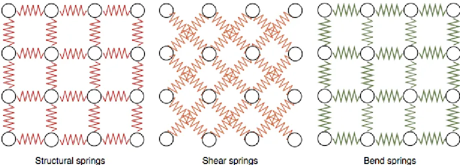
[image:11.612.101.561.412.577.2]The mass spring method follows a discrete model to simulate deformable objects. The method as the name implies use a network of point masses (or nodes) interconnected with massless springs. Each node is subject to both internal forces from the massless springs and external forces such as gravity, wind, etc. The springs are used to define the behavior of the cloth as well as dampening forces for stability. There are three kinds of springs [17] that may be defined. That is, structural springs, shear springs, and bend springs. Each following a skewed principle of Hooke’s law. By setting the spring constant for each of the different sprint types, material such as cotton, wool, and etc. can be simulated. The structural springs govern the stretchiness of the cloth, the shear springs makes sure that the cloth doesn’t appear to tear, and the bend springs are used to make sure the cloth doesn’t collapse on itself immediately upon simulation. The bend springs can be placed in any fashion, because it is just there to make sure the cloth doesn’t collapse to quickly on itself.
The springs are normally modeled as such,
fi =ks(|xij| −lij)
xij
|xij|
(3.1)
Wherefi is the force acing on point massi,xij is the diference between the two particless
position vectors,ksis the spring constant andlij is the original rest length.
The particles are governed by Newton’s second law
f =m¨x (3.2)
Wheremis the mass of each particle andf is the net force applied to the current particle. The net force f broken down into internal forces (massless springs) and external forces (gravity, wind, friction, etc.). x¨is the second derivative of the position with respect to time. Positions are then solved through a set of ordinary differential equations (ODEs) using a numerical scheme integrated over time to simulate the dynamic deformable behavior. The simplest method for numerical integration would be the tried and true Euler’s method.
vt+1 =vt+ ∆tf(xt, vt)/m (3.3)
xt+1=xt+ ∆tvt (3.4)
This is an explicit integration that can handle many cases, but when the provided timestep that is too small many problem come about in Euler’s method. In this case, Verlet integration [11] can be used over Euler’s method to solve this problem. Originally, Verlet integration was used to calculate the trajectory in molecular dynamics, but has been adapted for the use in video games’ physics simulation. As such, the method provides much more stability and much simpler to use than the Euler’s method. So in many cases, the following integration is used instead.
vt+1 = (xt+1−xt)/∆t. (3.6)
There are also implicit integration schemes that can be used in mass-spring models. [3]
3.3
Position Based Dynamics
Taking a step further, position based dynamics [15] offers a solution that allows for the direct manipulation of particle positions. This eliminates overshooting and energy gain problems we get with explicit integration with forces. Not only can these problem be avoided, other problems like oscillation and instability are also removed. To iterate, the main advantages in using position based dynamics cited from the original paper [15].
• Position based simulation gives control over explicit integration and removes the typical instability.
• Positions of vertices and parts of objects can directly be manipulated during the sim-ulation.
• The formulation we propose allows the handling of general constraints in the position based setting.
• The explicit position based solver is easy to understand and implement.
type solver where each constraint is handle individually leadings to slow propagation of information throughout the mesh. Visual artifacts like overly stretchy behavior can be seen for high resolution cloths.
3.3.1
Algorithm Overview
The following is the pseudo-code from the original [MHR*06] paper.
Algorithm 1Psuedo-code of position-based dynamics algorithm
1: procedurePBD
2: for allparticlesido
3: initializexi=x0i ,vi=vi0,wi =1/mi
4: end for
5: loop
6: for allverticesidov ←v+ ∆twifext(xi)
7: end for
8: dampVelocities(v1,...,vN)
9: for allverticesidop←xi+ ∆tvi
10: end for
11: for all verticesi dogenerateCollisionConstraints(xi ←p)
12: end for
13: repeat
14: projectConstraints(C1, ..., CM+Mcoll, p1...pN)
15: untilsolverIterations times
16: for all verticesi do
17: vi ←(pi−xi)/∆t
18: xi ←pi
19: end for
20: velocityUpdate(v1, ..., vN)
21: end loop
22: end procedure
WhereC1, ..., CM+Mcoll are all the constraints (both internal and collision constraints),
p1...pN are all the particles andv1, ..., vN are all the velocities.
can be provided in the cases where external forces or timesteps can cause instability to the simulation. This velocity is then integrated to generate new positions for each particle as shown in line (7). The interesting parts are in lines (9)-(11) where instead of springs that generate internal forces to maintain the cloth’s shape and behavior, constraints are used. These constraints are similar to springs in that k as a ”spring” constant is still used to describe the stiffness of the links between particles. However, constraints here directly manipulate the position to satisfy that ”stiffness” or even ”bend” factors (analogous to force-based bend springs). The same constraint structure are also used to solve collisions. The collision constraints are generated in step (8). While new positions are generated in line (7), they are modified until all constraints are satisfy. Once that happens, it is then where each particle is updated with a corresponding position and velocity.
3.3.2
Constraint Projection
When projecting constraints, both linear and angular momentum must be conserved. Muller’s method presents an equation that conserves both linear and angular momentum for internal constraints. The equation is
C(p+ ∆p)≈C(p) +∇pC(p)·∆p= 0 (3.7)
Wherepis the concatenation[pT1, ..., pTn]T. Cis the constraint function.
The focus is on∆pwhere we want to know how much we need to displace each point to satisfy all constraints. So after a few more derivations [16], the general formula for constraint projection is as follow
Where s is the scaling factor used with the given formula
s = C(p1, ..., pn) Σjwj|∇pjC(p1, ..., pn)|
2 (3.9)
With this many constraint functions can be used to generate a variety of materials. Further constraints that are used...
Distance Constraint
This constraint is a simple distant constraint for generic soft bodies.
C(p1, p2) =|p1−p2| −d (3.10)
Stretch Constraint
This constraint is analogous to structural springs in cloth. It is similar to the distance constraint.
Cstretch(p1, p2) =|p1−p2| −l0 (3.11)
Bend Constraint
This constraint is analogous to bend springs in cloth.
Cbend(p1, p2, p3, p4) = acos(
(p2−p1)×(p3−p1)
|(p2−p1)×(p3−p1)|
· (p2 −p1)×(p4−p1) |(p2 −p1)×(p4−p1)|
)−ϕ0
(3.12)
Self-Collision Constraint
Because position-based dynamics generalizes constraints, collision are also viewed as con-straints. This constraint is used self-collisions in cloth.
C(q, p1, p2, p3) = (q−p1)·
(p2−p1)×(p3−p1)
|(p2−p1)×(p3−p1)|
3.4
Graphics Pipeline
The graphics pipeline is a pipeline used to render a 3D scene into a 2D raster image. A 3D scene which is composed of a collection of primitives is sent through this pipeline in which it is responsible for space transformations, vertex shading, primitive generation, projection, clipping, fragment shading, and etc. On the GPU, these operations are mapped onto several stages on the hardware which are input assembler stage, vertex shader stage, geometry shader stage, rasterizer stage, pixel shader stage, and the output merger stage.
Over the years, fully programmable stages have been added to the originally fixed func-tion pipeline of the GPU. This allowed developers to dictate their own operafunc-tions for most stage in the pipeline. With the release of DirectX 11 last year, three new stages have been added to the graphics pipeline1. These three new stages allow for dynamic tessellation to be
done on the hardware adding unprecedented amount of detail to models without incurring much cost. Given a coarse mesh (also known as a control cage), this technique can contin-uously tessellate the model to give it higher resolution. This means developers no longer need to worry about transferring large amounts of data per frame to the graphics hardware to get highly detailed render images2.
The key motivations for hardware tessellation are
• Compression: By using tessellation, we reduce the amount of memory needed to store 3D assets. This is very important when every vertex in a model can hold a position, normal, tangent, texture coordinate(s), animation data, weight, and etc. The memory needed to hold a model with a lot of vertices can easily get out of hand. On the other hand when using tessellation, we can eliminate the number of vertices we needed to store by generating new vertices from a control cage. On the same note, with less vertices to be stored, more animation data can be created for better animations.
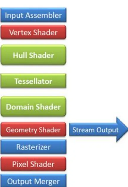
The current DirectX 11 graphics pipeline is as follow.
Figure 3.2: DirectX 11 graphics pipeline.
With the addition of three new stages to the pipeline, responsibilities of some shader stages have been shifted. While traditionally the vertex shader is responsible for space transformations when tessellation is enabled, the vertex shader only serves to transform vertices for animations in object space and other responsibilities are moved to the domain shader. In the following section, I will highlight the responsibilities of the new stages and also note the changes from the traditional pipeline.
1While this paper is only describing the stages illustrated in DirectX, analogous shader stages are also
available in OpenGL.
3.4.1
Hull Shader Stage
Since the graphics pipeline can now handle higher order surfaces, vertex data from the input assembler are viewed as control points. These control points can be used to generate bezier surfaces or even Catmull-Clark subdivision surfaces.
[image:20.612.166.461.406.504.2]Hull-Shader stage is a programmable shader stage that generates output control points from input control points passed in from the vertex-shader stage. The hull-shader is actually divided into two phase: one which operates on the control points and the other operates on the patch-constant. The control point phase is invoked once for each output control point and is responsible for transforming input control points. It is also used to specify the patch constant function for the patch-constant phase. The patch-constant phase is invoked once for per patch. It’s mainly responsible for specifying the edge tessellation factor which tells the tessellator stage how to subdivide the patch and the partitioning scheme for the tessellated patch.
Figure 3.3: Hull shader
3.4.2
Tessellator Stage
Using the tessellation factor (which specifies how many times to subdivide) and partition-ing scheme (which specifies how to subdivide), It takes a domain (quad, tri, or line) and generates primitives that can be rendered by the hardware (triangles, points, or lines).
3.4.3
Domain Shader Stage
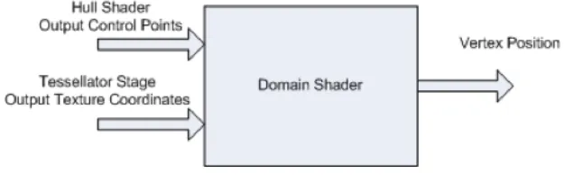
[image:21.612.151.469.359.456.2]Domain-Shader stage is a programmable shader stage that operates on the subdivided point generated by the tessellator stage. This stage is invoked once per tessellator stage output point. The output point is consumed and converted into a vertex. A set of UV coordinates are provided and depending on the input patch’s domain the output point is calculated differently. For a tri domain the output point are given in barycentric coordinate while a line is just a simple linear interpolation.
Figure 3.4: Domain shader
Once the output point has been calculated, the domain shader in this stage essentially takes over the responsibilities of the traditional vertex shader. It is charged with vertex transformations, per vertex lighting, and etc. Techniques like displacement mapping can be performed here. After the domain shader is complete, it continues down the pipe visiting the geometry shader stage, pixel shader stage, and etc.
3.4.4
Geometry Shader Stage
The geometry-shader stage is also a programmable shader stage. Introduced in DirectX 10, it is in charge of processing primitives. It is invoked once per primitive and it can be used to generate primitives or ignore incoming primitives. Unlike the vertex shader, the geometry shader can operate on multiple vertices depending on the primitive. The geometry shader can also choose to output an entirely different primitive type from the input primitive. That is, tristrip, linestrip, or pointlist. Once done processing, geometry may also be streamed out to a buffer in memory via the stream-output stage instead going to the fragment-shader stage.
3.4.5
Compute Shader
4. Proposed Solution
The goal is to map position based dynamics on to the GPU and at the same time take ad-vantage of hardware tessellation so high resolution cloth can be simulated a very little cost. To do so, some necessary steps must be taken into consideration in order to successfully implement this approach. The following issues must be addressed
• Information about the previous cloth simulation timestep is needed for numerical integration. This means we need some way to store this information.
• Due to the parallel nature of the GPU, when projecting constraints special care must be taken to ensure that no one vertex is being modified at the same time by any thread.
• Collision with other objects must be handled differently since accessing information about object might require the system to load data from the CPU onto the GPU. This may be a costly operation.
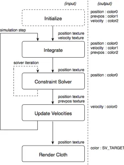
In this section I will present a multi-pass system that maps the position-based dynamics algorithm on to the GPU. The system works very much like a compositor system used to generate image-based effects like deferred shading or depth of field. The position based dynamic algorithm mentioned in an earlier section will be broken up into multiple pass. Each pass will operate on the particles in screen space and then the results are handed over to the next pass. This process is cycled for each simulation step repeatedly updating particle position and velocity.
data through the color semantics and from our next pass we simply use the previous render target’s texture as input. The texture coordinates from each vertex (or particle) will allow us to access the position and velocity information from that previous pass.
Even though I mentioned the use of a texture to store information, stream output stage of the pipeline may also be used to achieve this. But this requires much more processing at the vertex-shader stage then I intend for this solution and it would difficult to output multiple targets of information.
[image:24.612.185.435.308.640.2]The sections to follow will go into detail what each sequential pass of the system does.
4.1
Initialization
This is the first pass in the system and it is only invoked once at the beginning of the simulation. It’s sole responsibility is to initialize the state of the cloth. That is, the position, velocity and mass of each particle 1. One thing that must be mention about each pass is that tessellation is done for each. Though it may be expensive, it is needed because we do not operate at the pixel-shader stage in this system. The whole solution works at the domain-shader stage and/or geometry-shader stage.
At the domain-shader level, each particle is initialized with a position at rest and veloc-ity of zero.
Listing 4.1: Initialization domain shader
[ domain ( ” q u a d ” ) ]
DS OUTPUT B e z i e r D S ( HS CONSTANT DATA OUTPUT i n p u t ,
f l o a t 2 UV : S V D o m a i n L o c a t i o n ,
c o n s t O u t p u t P a t c h<HS OUTPUT , OUTPUT PATCH SIZE> p a t c h ) {
f l o a t 3 t o p M i d p o i n t = l e r p ( p a t c h [ 0 ] . p o s i t i o n , p a t c h [ 1 ] . p o s i t i o n , UV . x ) ;
f l o a t 3 b o t t o m M i d p o i n t = l e r p ( p a t c h [ 3 ] . p o s i t i o n , p a t c h [ 2 ] . p o s i t i o n , UV . x ) ;
f l o a t 3 o b j e c t p o s = l e r p ( t o p M i d p o i n t , b o t t o m M i d p o i n t , UV . y ) ;
/ / C l e a n up i n a c c u r a c i e s
f l o a t 3 s c r e e n p o s = o b j e c t p o s ;
/ / Image−s p a c e
f l o a t 2 uv ;
uv . x = 0 . 5 ∗ ( 1 + s c r e e n p o s . x ) ;
uv . y = 0 . 5 ∗ ( 1 − s c r e e n p o s . y ) ;
DS OUTPUT o u t p u t ;
o u t p u t . s c r e e n p o s = f l o a t 4 ( s c r e e n p o s . xy , 0 , 1 ) ;
o u t p u t . n o r m a l = f l o a t 3 ( 1 , 0 , 0 ) ;
o u t p u t . p o s i t i o n = mul ( f l o a t 4 ( o b j e c t p o s , 1 ) , g mWorld ) ;
r e t u r n o u t p u t ; }
4.2
Integration
In this pass, explicit integration is used to derive new positions and velocity from the pre-vious pass. In the case of the first simulation step, it takes as input from the initialization pass where velocity is zero and all particles are at rest. This process happens in the domain shader. Once completed, the information is render to a texture to be used as input for the next pass2.
Listing 4.2: Integration domain shader
[ domain ( ” q u a d ” ) ]
DS OUTPUT B e z i e r D S ( HS CONSTANT DATA OUTPUT i n p u t ,
f l o a t 2 UV : S V D o m a i n L o c a t i o n ,
c o n s t O u t p u t P a t c h<HS OUTPUT , OUTPUT PATCH SIZE> p a t c h ) {
f l o a t 3 t o p M i d p o i n t = l e r p ( p a t c h [ 0 ] . p o s i t i o n , p a t c h [ 1 ] . p o s i t i o n , UV . x ) ;
f l o a t 3 b o t t o m M i d p o i n t = l e r p ( p a t c h [ 3 ] . p o s i t i o n , p a t c h [ 2 ] . p o s i t i o n , UV . x ) ;
f l o a t 3 o b j e c t p o s = l e r p ( t o p M i d p o i n t , b o t t o m M i d p o i n t , UV . y ) ;
/ / C l e a n up i n a c c u r a c i e s
f l o a t 3 s c r e e n p o s = o b j e c t p o s ;
/ / Image−s p a c e
f l o a t 2 uv ;
uv . x = 0 . 5 ∗ ( 1 + s c r e e n p o s . x ) ;
uv . y = 0 . 5 ∗ ( 1 − s c r e e n p o s . y ) ;
DS OUTPUT o u t p u t ;
o u t p u t . s c r e e n p o s = f l o a t 4 ( s c r e e n p o s . xy , 0 , 1 ) ;
o u t p u t . n o r m a l = f l o a t 3 ( 1 , 0 , 0 ) ;
o u t p u t . uv = uv ;
f l o a t 3 p o s i t i o n = P o s i t i o n M a p . S a m p l e L e v e l ( g s a m p l e L i n e a r , uv , 0 ) . xyz ;
f l o a t 3 v e l o c i t y = V e l o c i t y M a p . S a m p l e L e v e l ( g s a m p l e L i n e a r , uv , 0 ) . xyz ;
f l o a t i n v e r s e M a s s = P o s i t i o n M a p . S a m p l e L e v e l ( g s a m p l e L i n e a r , uv , 0 ) . w ; f l o a t 3 p r e v p o s = p o s i t i o n ;
/ / E x t e r n a l f o r c e s − g r a v i t y
v e l o c i t y += g f E l a p s e d T i m e ∗ f l o a t 3 ( 0 . 0 f , 1 0 . 0 f , 0 . 0 f ) ∗ i n v e r s e M a s s ;
p o s i t i o n += v e l o c i t y ∗ g f E l a p s e d T i m e ;
o u t p u t . p o s i t i o n = p o s i t i o n ;
o u t p u t . v e l o c i t y = v e l o c i t y ;
o u t p u t . p r e v p o s = p r e v p o s ;
r e t u r n o u t p u t ; }
In the same pass, velocity dampening can be introduced here too.
4.3
Constraint Projection
In this pass, particles are projected for a given set of constraints. Position estimates are made by each constraint in order to satisfy all constraints. For the information to properly propagate, multiple iteration of this pass may be needed in order to do so. The first set of constraints are the internal constraints of the cloth. Up until now, particles have been processed independently of each other, this works well under the parallel architecture of the GPU. However, with internal constraint in this scenario, more than one particle are being manipulated at once.
For this, constraints must be handle differently. In this situation, that means no one particle can be processed at the same time by any of the GPU threads. In essence, we have to come up with a plan to have multiple independent constraints run in parallel.
Figure 4.2: Constraint groups.
A total of eight groups will be needed to be processed independent of each other. Since, we are dealing with a rectangular cloth certain assumption can be made about neighbor-ing particles and primitives can be distneighbor-inguished procedurally for each group. This will guarantees that constraints will not overwrite the results of other constraints.
Listing 4.3: Classify edge to group for the constraint solver
b o o l F i n d G r o u p ( DS OUTPUT I n [ 3 ] , i n t g r o u p ) { f l o a t 2 min = I n [ 0 ] . uv ;
f l o a t 2 max = I n [ 0 ] . uv ;
i n t v e r t 0 , v e r t 1 ; b o o l f o u n d = f a l s e ;
f o r (i n t i = 0 ; i < 3 ; ++ i ) {
/ / F i n d t h e minimum
i f ( I n [ i ] . uv . y < min . y ) { min . y = I n [ i ] . uv . y ; }
/ / F i n d t h e maximum
i f ( I n [ i ] . uv . x > max . x ) { max . x = I n [ i ] . uv . x ; }
i f ( I n [ i ] . uv . y > max . y ) { max . y = I n [ i ] . uv . y ; } }
/ / Now t o f i n d o u t w h i c h g r o u p t h i s t r i a n g l e i s i n . . .
i f ( fmod ( max . y + 0 . 0 1 f , ( max . y − min . y ) ∗ 2 ) > 0 . 0 2 f ) {
i f ( g r o u p == 1 ) { r e t u r n t r u e ; } }
i f ( fmod ( max . x + 0 . 0 1 f , ( max . x − min . x ) ∗ 2 ) > 0 . 0 2 f ) {
i f ( g r o u p == 2 ) { r e t u r n t r u e ; } }
i f ( fmod ( max . y + 0 . 0 1 f , ( max . y − min . y ) ∗ 2 ) < 0 . 0 2 f ) {
i f ( g r o u p == 3 ) { r e t u r n t r u e ; } }
i f ( fmod ( max . x + 0 . 0 1 f , ( max . x − min . x ) ∗ 2 ) < 0 . 0 2 f ) {
i f ( g r o u p == 4 ) { r e t u r n t r u e ; } }
r e t u r n f a l s e ; }
In this same pass, collision constraint must also be enforced. This can be done without having to partition particles into groups since they operate independently of each other. Though this must happen after all internal constraints have been satisfied to prevent colli-sions that may occur while trying to satisfy non-collision constraints.
types of collision primitives can be passed in as an array into the shader. The shader will it-erate through the list and figure out easily whether or not there is a collision. More accurate collision detection however will require the developer to load an entire meshes into mem-ory and onto the GPU for processing. This can be very costly depending on how detailed the mesh is. An alternative solution that can be used instead is an image-based collision detection approach presented by [23].
This approach utilizes layers of depth maps to detect collisions with other objects. This is much cheaper as texture look-ups are much faster than intersection tests with meshes.
Listing 4.4: Part of the constraint solver geometry shader
GS OUTPUT o u t p u t ;
/ / F i n d d i s t a n c e b e t w e e n t w o p o i n t s f o r t h e quad s i z e
f l o a t s i z e = l e n g t h ( I n [ 0 ] . s c r e e n p o s . xyz − I n [ 1 ] . s c r e e n p o s . xyz ) / 4 ;
/ / F i n d t h e n o d e g r o u p
i n t n o d e 0 = 0 ;
i n t n o d e 1 = 1 ;
i n t g r o u p = g f G r o u p ;
i f ( F i n d G r o u p ( I n , g r o u p ) ) {
/ / f i n d t h e h o r i z o n t a l o r f i n d t h e v e r t i c a l l i n e
i f ( ( g r o u p == 1 ) | | ( g r o u p == 3 ) ) {
/ / v e r t i c a l
f o r (i n t n = 0 ; n < 3 ; ++n ) {
i f ( I n [ n ] . uv . x == I n [ ( n + 1 ) % 3 ] . uv . x ) { n o d e 0 = n ;
n o d e 1 = ( n + 1 ) % 3 ;
}
}
} e l s e {
/ / h o r i z o n t a l
i f ( I n [ n ] . uv . y == I n [ ( n + 1 ) % 3 ] . uv . y ) { n o d e 0 = n ;
n o d e 1 = ( n + 1 ) % 3 ;
}
}
}
f l o a t k s t = 0 . 7 f ;
f l o a t massLSC = 1 . 0 f ;
f l o a t r e s t L e n g t h = l e n g t h ( I n [ n o d e 0 ] . o r i g i n a l − I n [ n o d e 1 ] . o r i g i n a l ) ;
f l o a t r e s t L e n g t h S q u a r e d = r e s t L e n g t h ∗ r e s t L e n g t h ;
i f( massLSC > 0 . 0 f ) {
f l o a t 3 p o s i t i o n 0 = I n [ n o d e 0 ] . p o s i t i o n ;
f l o a t 3 p o s i t i o n 1 = I n [ n o d e 1 ] . p o s i t i o n ;
f l o a t i n v e r s e M a s s 0 = I n [ n o d e 0 ] . i n v e r s e M a s s ;
f l o a t i n v e r s e M a s s 1 = I n [ n o d e 1 ] . i n v e r s e M a s s ;
f l o a t 3 d e l = p o s i t i o n 1 − p o s i t i o n 0 ;
f l o a t l e n = d o t ( d e l , d e l ) ;
f l o a t k = ( ( r e s t L e n g t h S q u a r e d − l e n ) / ( massLSC ∗ ( r e s t L e n g t h S q u a r e d + l e n ) ) ) ∗ k s t ; p o s i t i o n 0 = p o s i t i o n 0 − d e l ∗ ( k ∗ i n v e r s e M a s s 0 ) ;
p o s i t i o n 1 = p o s i t i o n 1 + d e l ∗ ( k ∗ i n v e r s e M a s s 1 ) ;
p o s i t i o n [ n o d e 0 ] = p o s i t i o n 0 ;
p o s i t i o n [ n o d e 1 ] = p o s i t i o n 1 ;
}
/ / Out t h e r e s u l t s i n q u a d s
f o r (i n t i = 0 ; i < 3 ; ++ i ) {
i f ( ( i ! = n o d e 0 ) && ( i ! = n o d e 1 ) ) { c o n t i n u e; }
o u t p u t . s c r e e n p o s = I n [ i ] . s c r e e n p o s + f l o a t 4 (−s i z e , −s i z e , 0 , 0 ) ;
o u t p u t . n o r m a l = I n [ i ] . n o r m a l ;
o u t p u t . uv = I n [ i ] . uv ;
o u t p u t . p o s i t i o n = p o s i t i o n [ i ] ;
T r i S t r e a m . Append ( o u t p u t ) ;
o u t p u t . s c r e e n p o s = I n [ i ] . s c r e e n p o s + f l o a t 4 (−s i z e , s i z e , 0 , 0 ) ;
o u t p u t . n o r m a l = I n [ i ] . n o r m a l ;
o u t p u t . uv = I n [ i ] . uv ;
o u t p u t . p o s i t i o n = p o s i t i o n [ i ] ;
T r i S t r e a m . Append ( o u t p u t ) ;
o u t p u t . s c r e e n p o s = I n [ i ] . s c r e e n p o s + f l o a t 4 ( s i z e , s i z e , 0 , 0 ) ;
o u t p u t . n o r m a l = I n [ i ] . n o r m a l ;
o u t p u t . uv = I n [ i ] . uv ;
o u t p u t . p o s i t i o n = p o s i t i o n [ i ] ;
T r i S t r e a m . Append ( o u t p u t ) ;
T r i S t r e a m . R e s t a r t S t r i p ( ) ; / / t o e n d t h e t r i a n g l e
/ / s e c o n d t r i a n g l e
o u t p u t . s c r e e n p o s = I n [ i ] . s c r e e n p o s + f l o a t 4 (−s i z e , −s i z e , 0 , 0 ) ;
o u t p u t . n o r m a l = I n [ i ] . n o r m a l ;
o u t p u t . uv = I n [ i ] . uv ;
o u t p u t . p o s i t i o n = p o s i t i o n [ i ] ;
T r i S t r e a m . Append ( o u t p u t ) ;
o u t p u t . s c r e e n p o s = I n [ i ] . s c r e e n p o s + f l o a t 4 ( s i z e , −s i z e , 0 , 0 ) ;
o u t p u t . n o r m a l = I n [ i ] . n o r m a l ;
o u t p u t . uv = I n [ i ] . uv ;
o u t p u t . p o s i t i o n = p o s i t i o n [ i ] ;
T r i S t r e a m . Append ( o u t p u t ) ;
o u t p u t . n o r m a l = I n [ i ] . n o r m a l ;
o u t p u t . uv = I n [ i ] . uv ;
o u t p u t . p o s i t i o n = p o s i t i o n [ i ] ;
T r i S t r e a m . Append ( o u t p u t ) ;
T r i S t r e a m . R e s t a r t S t r i p ( ) ; / / t o e n d t h e t r i a n g l e
}
} e l s e {
/ / E m i t e d g e s and c o r n e r s o n l y .
i f ( g r o u p == 1 ) {
f o r (i n t i = 0 ; i < 3 ; ++ i ) {
i f ( I n [ i ] . uv . y == 1 . 0 f ) {
E m i t P o i n t ( I n [ i ] , T r i S t r e a m , s i z e ) ;
}
}
} e l s e i f ( g r o u p == 3 ) {
f o r (i n t i = 0 ; i < 3 ; ++ i ) {
i f ( ( I n [ i ] . uv . y == 1 . 0 f ) | | ( I n [ i ] . uv . y == 0 . 0 f ) ) { E m i t P o i n t ( I n [ i ] , T r i S t r e a m , s i z e ) ;
}
}
} e l s e i f ( g r o u p == 2 ) {
f o r (i n t i = 0 ; i < 3 ; ++ i ) {
i f ( I n [ i ] . uv . x == 1 . 0 f ) {
E m i t P o i n t ( I n [ i ] , T r i S t r e a m , s i z e ) ;
}
}
} e l s e i f ( g r o u p == 4 ) {
f o r (i n t i = 0 ; i < 3 ; ++ i ) {
i f ( ( I n [ i ] . uv . x == 1 . 0 f ) | | ( I n [ i ] . uv . x == 0 . 0 f ) ) { E m i t P o i n t ( I n [ i ] , T r i S t r e a m , s i z e ) ;
}
}
T r i S t r e a m . R e s t a r t S t r i p ( ) ; / / t o e n d t h e t r i a n g l e
}
}
4.4
Velocity Update
The final pass of the simulation. In this pass, velocity will be updated according to the how much the particle has been displaced since the last simulation step. This means that the previous velocity will have no longer have any influence for the proceeding simulation steps. This pass is mainly to account for friction and restitution coefficients of colliding particles. If not handled correctly, the cloth will slide along other objects without stopping. Once completed, the new velocity will be used in the simulation step’s integration pass.
Listing 4.5: Velocity update domain shader
[ domain ( ” q u a d ” ) ]
DS OUTPUT B e z i e r D S ( HS CONSTANT DATA OUTPUT i n p u t ,
f l o a t 2 UV : S V D o m a i n L o c a t i o n ,
c o n s t O u t p u t P a t c h<HS OUTPUT , OUTPUT PATCH SIZE> b e z p a t c h ) {
f l o a t 3 t o p M i d p o i n t = l e r p ( b e z p a t c h [ 0 ] . p o s i t i o n , b e z p a t c h [ 1 ] . p o s i t i o n , UV . x ) ;
f l o a t 3 b o t t o m M i d p o i n t = l e r p ( b e z p a t c h [ 3 ] . p o s i t i o n , b e z p a t c h [ 2 ] . p o s i t i o n , UV . x ) ;
f l o a t 3 o b j e c t p o s = l e r p ( t o p M i d p o i n t , b o t t o m M i d p o i n t , UV . y ) ;
/ / C l e a n up i n a c c u r a c i e s
f l o a t 3 s c r e e n p o s = o b j e c t p o s ;
/ / Image−s p a c e
f l o a t 2 uv ;
uv . x = 0 . 5 ∗ ( 1 + s c r e e n p o s . x ) ;
DS OUTPUT o u t p u t ;
o u t p u t . s c r e e n p o s = f l o a t 4 ( s c r e e n p o s . xy , 0 , 1 ) ;
o u t p u t . n o r m a l = f l o a t 3 ( 1 , 0 , 0 ) ;
o u t p u t . uv = uv ;
f l o a t 3 p o s i t i o n = P o s i t i o n M a p . S a m p l e L e v e l ( g s a m p l e L i n e a r , uv , 0 ) . xyz ;
f l o a t 3 p r e v p o s = P r e v i o u s P o s i t i o n M a p . S a m p l e L e v e l ( g s a m p l e L i n e a r , uv , 0 ) . xyz ;
f l o a t v e l o c i t y C o r r e c t i o n C o e f f i c i e n t = 1 . 0 f ;
f l o a t d a m p i n g F a c t o r = 0 . 2 f ;
f l o a t v e l o c i t y C o e f f i c i e n t = ( 1 . f − d a m p i n g F a c t o r ) ; f l o a t 3 d i f f e r e n c e = p o s i t i o n − p r e v p o s ;
f l o a t 3 v e l o c i t y = d i f f e r e n c e ∗ v e l o c i t y C o e f f i c i e n t ∗ 1 . f / g f E l a p s e d T i m e ;
o u t p u t . v e l o c i t y = v e l o c i t y ;
r e t u r n o u t p u t ; }
4.5
Render Cloth
The final render pass renders the actual cloth. Taking the position texture from the simula-tion, each vertex does a look-up into the texture and is displaced in world space. Normals can be derived by sampling neighboring pixel positions. Since the cloth is always facing the eye, the normals are always positive in view space.
Listing 4.6: Render cloth domain shader
[ domain ( ” q u a d ” ) ]
DS OUTPUT B e z i e r D S ( HS CONSTANT DATA OUTPUT i n p u t ,
f l o a t 2 UV : S V D o m a i n L o c a t i o n ,
c o n s t O u t p u t P a t c h<HS OUTPUT , OUTPUT PATCH SIZE> p a t c h ) {
f l o a t 3 b o t t o m M i d p o i n t = l e r p ( p a t c h [ 3 ] . p o s i t i o n , p a t c h [ 2 ] . p o s i t i o n , UV . x ) ;
f l o a t 3 o b j e c t p o s = l e r p ( t o p M i d p o i n t , b o t t o m M i d p o i n t , UV . y ) ;
/ / C l e a n up i n a c c u r a c i e s
f l o a t 3 s c r e e n p o s = o b j e c t p o s ;
/ / Image−s p a c e
f l o a t 2 uv ;
uv . x = 0 . 5 ∗ ( 1 + s c r e e n p o s . x ) ;
uv . y = 0 . 5 ∗ ( 1 − s c r e e n p o s . y ) ;
DS OUTPUT o u t p u t ;
o u t p u t . n o r m a l = f l o a t 3 ( 1 , 0 , 0 ) ;
o u t p u t . uv = uv ;
f l o a t 3 p o s i t i o n = P o s i t i o n M a p . S a m p l e L e v e l ( g s a m p l e L i n e a r , uv , 0 ) . xyz ;
o u t p u t . p o s i t i o n = mul ( f l o a t 4 ( p o s i t i o n , 1 ) , g m V i e w P r o j e c t i o n ) ;
r e t u r n o u t p u t ; }
4.6
Issues
Some issues have not been addressed yet, though it is not the focus of this thesis, will have a brief discussion regarding the subject.
4.6.1
Attachments
4.6.2
Tearing
Tearing is not supported in this solution, but ideas for tearing can be implemented at the render pass of the cloth. By specifying a stress threshold for each particle, at the geometry-shader stage of rendering developer can choose to ignore or shrink primitives that are pass the threshold to simulate tearing.
4.6.3
Self-Collision
5. Deliverables and Evaluations
5.1
Deliverables
The main deliverable from this thesis will be a position-based dynamic solution imple-mented on completely on the GPU that utilizes hardware tessellation to produce high res-olution cloth. It will also be suitable for interactive use. The sres-olution and results will be detailed in my thesis write-up and defense.
5.2
Evaluation
6. Implementation Details
There were many challenges throughout this thesis. The following section will outline in particular the roadblocks that I encountered while implementing the solution.
6.1
Encoding Position and Velocity Information
One of the first roadblocks that I encountered was trying to encode position and velocity information onto a render texture. This approach is similar to deferred shading techniques in which information about the scene (normal, depth, diffuse) is rendered out to be handled later as a post process compositor. Naturally, this same approach should work in my simu-lation as I am also encoding information in screen-space onto a render texture. Though this sort of encoding normally happens at the pixel-shader stage, in my solution this happens at the domain-shader stage and/or geometry-shader stage.
I attempted to encode the texture from the domain-shader stage and geometry-shader stage, but this lead to shrinking of the cloth. This is due to the way the graphics hardware handle vertices that enters the pixel-shader stage. As some vertices might not land exactly on a pixel in which the hardware will interpolate between neighboring vertices to fill that pixel. This effect was most apparent at the edges of the cloth.
6.2
Managing Render Targets
One of the main issues I had was trying to keep data persistent between simulations steps. Because each simulation step relies on the data from the previous step, the data must be rendered out to a texture. The problems comes when some render pass need to read and write to the same texture. Since a render target can not be read from and written to simul-taneously, this is impossible. I instead created a series of ”swap” targets for each persistent data texture. This includes: position, previous position and velocity information. Just like double buffering techniques, this allowed me to write to a ”back” buffer and swap out the old buffer when the new data is needed at the beginning of each render pass.
With the ”swap” targets in place, I thought this would fix the data persistent issue, but I was losing data at each simulation step. This problem was hard to track down. Several tests were conducted to figure out what was wrong with the swapping and the shaders, but I couldn’t find anything wrong with the system. I was debugging the problem for almost two weeks, but I had no luck with it. So I had to look at other areas of the solution that might be cause of the problem. The topic of texture filtering came up in my investigation. This could very well be the source of the problem. I started playing with the texture sampling settings and sure enough a combination of filtering and wrapping options was the problem. I figured out that point sampling and simple clamping worked best in my solution.
The issue doesn’t stop there though. I had a lot of precision problems in my solution where at time nodes would be on top of each other. This was a pretty easy issue to solve. I only needed to increase the precision of the render texture format from half-floats to full 32-bit floating point precision texture.
6.3
Parallelizing the Constraint Solver
it gets tricky. The issue of how to parallelize the solution comes up. At first, I naively processed each constraint in the geometry shader, but results were being overwritten by other constraints that are trying to satisfy their own rules. This led to stretching of the first row of triangles while all other triangle stayed at rest when gravity was applied.
7. Results
I have successfully mapped position-based dynamics over to the GPU for rectangular cloths. The solution was tested on two machines with different graphics hardware. The first one has an Intel(R) Core(TM) Quad @ 3.00GHz using 2.00GB RAM with an ATI Radeon HD 5800 Series. The second is a Intel(R) Core(TM) i7 @ 2.80GHz using 4.00GB RAM with an NVIDIA GeForce GTX 480. All results are obtained from these two ma-chines.
As the main benchmark is performance, Table 1 gives an overview of the general per-formance of the simulation with respect to the complexity of the cloth. Interestingly, as the complexity is increased, the drop in performance wasn’t that significant. This was unex-pected as we susunex-pected the frame-rate would have plummeted as the particles (or vertices) went over 10,000. After careful examination and tests, we conclude that because all the particles were able to run in parallel on the hardware we were able to get such good per-formance giving us only a slight drop in perper-formance with respect to the complexity of the cloth.
Node(s) ATI Radeon HD 5800 Series NVIDIA GeForce GTX 480 8x8 482.65 807.65
16x16 481.28 782.98 32x32 427.62 778.17 45x45 350.27 753.73 50x50 322.13 675.48 55x55 298.18 600.23 64x64 254.90 454.52 128x128 92.96 180.39
Texture resolution ATI Radeon HD 5800 series NVIDIA GeForce GTX 480 128x128 30.0 30.0
256x256 30.0 50.0 512x512 128.0+ 128.0+
Table 7.2: Maximum tessellation level supported.
Aside from the complexity of the cloth, there are other variables that dictate the per-formance of the simulation. One of the main variables that really affected the perper-formance iwas the resolution of the render texture used to encode position and velocity information. Like any compositor system used for post-processing effects, the pixel fill rate is a con-stant cost that cannot be sped up. In Table 2 we show the performance results from using different resolutions for the render texture.
In order to simulate higher resolution cloth, the render texture must also increase in resolution. In the next table we show the maximum resolution that each render texture can handle.
At each simulation step, the algorithm goes through multiple render passes and a mini-mum of three passes must occur for one step. That is, one pass for integration, one pass for constraint projections and a final pass to adjust the final velocities to be used in the next sim-ulation step. The main concern here is the constraint solver pass. This pass must be done several times to stabilize the cloth. As mentioned earlier, information propagates slowly with position-based dynamics’ Gauss-Seidel type solver which is why multiple passes are needed depending on the complexity of the cloth. To stabilize the simulation, the cloth thus requires multiple passes, but that also means more cost in performance as each pass adds a constant cost that cannot be sped up. Next table shows the cost performance per solver iteration and also another table that shows the minimum number of iterations to stabilize a cloth for multiple resolutions.
Resolution Iteration(s) ATI Radeon HD 5800 Series NVIDIA GeForce GTX 480
8x8 1 525.65 2605.97
16x16 1 491.68 2504.86 32x32 1 472.95 2214.14 45x45 1 421.73 1707.32 50x50 1 399.94 1450.95 55x55 1 380.55 1258.30 64x64 1 336.65 973.05 128x128 1 153.41 303.56
8x8 2 357.51 2147.0
16x16 2 339.83 2003.71 32x32 2 330.96 1642.33 45x45 2 297.16 1187.15 50x50 2 281.15 981.70 55x55 2 257.81 854.45 64x64 2 235.25 656.34 128x128 2 109.27 223.87
8x8 2 274.73 1989.45
16x16 3 260.89 1885.14 32x32 3 253.69 1304.69 45x45 3 229.02 904.54 50x50 3 216.64 750.90 55x55 3 205.67 650.30 64x64 3 198.12 495.39 128x128 3 84.93 176.24
8x8 5 184.60 1675.24
[image:45.612.103.509.146.622.2]16x16 5 176.69 1458.93 32x32 5 173.37 925.93 45x45 5 156.98 610.37 50x50 5 148.64 501.92 55x55 5 140.78 435.29 64x64 5 124.28 337.62 128x128 5 58.73 123.12
Figure 7.1: Iteration performance results - ATI Radeon HD 5800 Series
Node(s) Iteration(s) 8x8 1 16x16 2 32x32 2 64x64 3 128x128 4
Table 7.4: Number of iteration for stability
the test were done on different hardware, the paper is still fairly recent. Our solution’s performance are comparable if not better than the results that were published. Though we must also take into account that we have more updated hardware. I would be interested in comparing the results using identical hardware.
[image:46.612.252.369.364.451.2]Figure 7.2: Iteration performance results - NVIDIA GeForce GTX480
vertices can run at rates of over 100 frames per second. The GPU was able to improve the performance dramatically when compared to the CPU solution of the original paper.
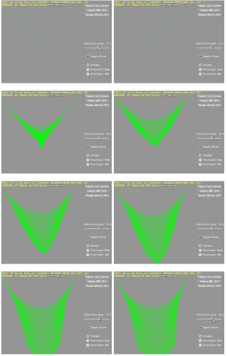
The next metric for evaluation is the stability of the simulation itself. In this section, multiple tests were done to put the simulation under stress. For example, stretching the cloth well beyond it’s rest length, extreme gravity, extreme impulse forces, and etc. The following case will be tested and the results will be shown below.
• Case 1: All nodes will be set to the same initial position except for anchor nodes.
• Case 2: All nodes will be stretched beyond their resting length between neighboring nodes.
• Case 3: Extreme gravity will be applied throughout the simulation.
• Case 4: Other external forces will stress the stability of the cloth.
8. Conclusion and Future Work
The use of more GPU-based solution have been sought by many developers in different fields and I hope this research will help people in my field of real-time graphics. I have presented a GPU implementation of the position-based dynamics method for cloth simula-tion using hardware tessellasimula-tion. It is easy to integrate and inherits the many advantages of the original CPU method. It is stable and efficient for real-time use. Naturally, there’s still a lot of improvements and optimizations that can done.
First and foremost, I’d like to extend the solution to handle non-structured meshes. The problem to be solved here is how do we handle all the constraints in parallel for non-structured meshes. This problem actually roots to the early courses of computer science. It is a graph coloring problem or to be more specific edge coloring problem. Essentially, all constraints or edges must be colored such that no two adjacent edges share the same color. By solving this problem, it will take us one step closer to our goal. The next step is figuring out how to do the coloring on-the-fly and on the GPU.
The next improvement is to minimize the resolution of the render textures, but still be able to support high resolution models. A technique described in GPU Gems 3’s ”Using the Geometry Shader for Compact and Variable-Length GPU Feedback” [18] article by Franck Diard explains how to encode data using geometry-shader stage’s point-stream. This is a very useful article in that it will allow us to encode position and velocity information to just one pixel instead of the point sprite approach that’s being employed. This will reduce the number duplicate information that’s being rendered to the texture and also reduce the size of the texture saving us both processing and rendering cost.
more deferred approach might be able suffice where we instead create a sky-box like depth map to test for collision.
Bibliography
[1] MSDN documentation - DirectX 11 documentation, 2011. http://msdn.
microsoft.com/en-us/library/ff476080(VS.85).aspx.
[2] D. Baraff and A. Witkin. Large steps in cloth simulation. SIGGRAPH ’98 Proceed-ings of the 25th annual conference on Computer graphics and interactive techniques, 1998. http://dx.doi.org/10.1145/280814.280821.
[3] D. Breen, D. House, and M. Wozny. Predicting the drape of woven cloth using interacting particles. Proceeding in SIGGRAPH ’94 Proceedings of the 21st an-nual conference on Computer graphics and interactive techniques, 1994. http:
//portal.acm.org/citation.cfm?doid=192161.192259.
[4] R. Bridson, S. Marino, and R. Fedkiw. Simulation of clothing with folds and wrinkles.
Proceedings of SIGGRAPH ’05 ACM SIGGRAPH 2005 Courses, 2005. http://
dx.doi.org/10.1145/1198555.1198573.
[5] Bullet. Bullet Physics Library. http://bulletphysics.org/.
[6] Tonnesen D. Spatially Coupled Particle Systems. Particle System Modeling, Anima-tion, and Physically Based Techniques, 1992.
[7] M. Desbrun, P. Schrder, and A. Barr. Interactive animation of structured deformable objects. Proceedings of the 1999 conference on Graphics interface, 1999.
[8] S. Green. GPU cloth simulation. http://developer.nvidia.com/
[9] Havok. Havok Cloth. http://www.havok.com/index.php?page=
havok-cloth.
[10] Monaghan J. Smoothed particle hydrodynamics. Annual Rev. Astron. Physics, 1992.
[11] T. Jakobsen. Advanced character physics, 2001. http://www.gamasutra.
com/resource_guide/20030121/jacobson_pfv.htm.
[12] D. Macri. Simulating Cloth for 3D Games, 2010. http://software.intel.
com/en-us/articles/simulating-cloth-for-3d-games/.
[13] M. Muller. Hierarchical Position Based Dynamics. Proceedings of Virtual Reality Interactions and Physical Simulations (VRIPhys2008), 2008.
[14] M. Muller, J. Dorsey, L. McMillan, R. Jagnow, and B. Cutler. Stable real-time de-formations. Proceedings of the 2002 ACM SIGGRAPH/Eurographics symposium on Computer animation), pages 49–54, 2002.
[15] M. Muller, B Heidelberger, M. Hennix, and J. Ratcliff. Position based dynam-ics. Journal of Visual Communication and Image Representation, 18(2), April 2007.
http://dx.doi.org/10.1016/j.jvcir.2007.01.005.
[16] M. Mller, J. Doug, Nils Theurey, and J. Stam. Real Time Physics, 2008. http:
//www.matthiasmueller.info/realtimephysics/.
[17] A. Nealen, M. Muller, R. Keiser, E. Boxerman, and M. Carlson. Physically based deformable models in computer graphics. Eurographics 2005 state of the
art report, 2005. http://www.matthiasmueller.info/publications/
egstar2005.pdf.
[18] Hubert Nguyen. GPU Gems 3. Addison-Wesley Professional, 2007.
[19] NVIDIA. PhysX Physics Engine. http://developer.nvidia.com/
[20] J. F. O’Brien and Hodgins J. K. Graphical modeling and animation of brittle fracture.
Proceedings of the 26th annual conference on Computer graphics and interactive
techniques, 1999.
[21] J. Rodriguez-Navarro and A. Susin. Non Structured Meshes for Cloth GPU Simula-tion using FEM. 3rd. Workshop in Virtual Reality, Interactions, and Physical Simula-tions (VRIPHYS’06), 2006.
[22] D. Terzopoulos, J. Platt, A. Barr, and K. Fleischer. Elastically deformable models.
Proceedings of SIGGRAPH ’87 Proceedings of the 14th annual conference on
Com-puter graphics and interactive techniques, 21(4), 1987. http://dx.doi.org/
10.1145/37402.37427.
[23] P. Volino and N. Magnenat-Thalmann. Comparing Efficiency of Integration Methods for Cloth Animation. Proceedings of Computer Graphics International (CGI)), pages 265–274, 2001.
[24] C. Zeller. Cloth simulation on the GPU. Proceeding in SIGGRAPH ’05 ACM
SIG-GRAPH 2005 Sketches, 2005. http://portal.acm.org/citation.cfm?