209
Study the Effect of Different Media Flow Speed
using Computational Simulation of AFM for two
Dimensional Models
Atul Singh Pathania, Sushil Mittal, Arun KumarAbstract— Abrasive Flow machining (AFM) also called Abrasive machining process which helps in achieving high level of surface finish and material removal rate from internal complex workpiece geometries after the machining operation. Concentration of abrasive, Abrasive size, extrusion pressure, media flow rate, number of strokes, media viscosity, strain rate and velocity are the factors which affect quality surface finish and MRR. Mathematical modelling, experimental results and computational simulation helps in improving the performance of Abrasive flow machining. This paper focuses mathematical model and computational simulation for the internal surface irregularities and effect of parameters with different media flow velocity. Computational Fluid dynamics (CFD) simulation was executed using commercial codes software available ANSYS FLUENT. CFD used numerical and algorithms methods (discrete counterparts of the governing equation) to analysis and get solution to the fluid flow problem. The fluid is assumed to be Newtonian fluid and type of flow should be steady, laminar and incompressible. Fluent Multiphase Mixture model for two phases was taken in account with secondary phase as continuous. The base media consist of Silly putty (Polyborosiloxane) and Silicon Carbide for the analysis.
Index Term— Abrasives, AFM, Axisymmetric, CFD, MRR, Multiphase model, Surface roughness. —————————— ——————————
1
I
NTRODUCTION FM stands for Abrasive Flow Machining also called Non-conventional finishing process used for neaten and smoothen rough edges, radius, holes, cavities, slots and polish highly complex structures and geometry but with low amount of material removal rate. AFM comes in existence in the beginning of year 1960 by Extrude Hone Corporation, USA [1]. Surface finish is the prime requirement for different application in industries and research area. Traditional machining process like grinding and polishing are not able to fulfill demands. Industries now days investing large proportion of money to get the desired surface finish. The Polymer which has property of both combined high viscosity/elasticity in nature and media abrasive particles are mixed in proportion and extruded under high pressure to get the desired surface finish. AFM is used for finishing interior surface by flowing abrasive media through the work piece, it is a type of surface finish process. AFM is used for finishing interior surface by using flowing abrasive media through the work piece, it is a type of surface finish process. The type of fluid used is highly viscous in nature having property like putty or dough. AFM are of three types which are described in the literature: one-way process [2], two-way process [3] and orbital AFM [4]. The medium forced or thrust out with the help of hydraulic or mechanical process from the upper filled hydraulic cylindrical chamber to the empty hydraulic chambered through narrow passage with the pistonmechanism and then it passes the workpiece surface. Some of the further research and development work on the basis of various process and response parameters are studied to optimize the material removal rate, surface finish and made this finishing process more advanced and better are completely reviewed in this paper. In et al. [5] considered the impact of process parameter on surface finish by enhancing the concentration of magnetic flux. They studied the weight of cylindrical workpiece (STS304) and check its micro-diameter. In the initial state rate of change of roundness was enhanced because roughness (unevenness) was more during that portion of time. They have worked on modified MAF setup (Magnetic Abrasive finishing). The concentration of magnetic flux was enhanced by simply adding yoke part (SS41-Steel type) in Fe-Nd-B type permanent magnet. The abrasive used in the experiment consist of diamond paste, iron magnetic particles (powder form) and grinding fluid (binder). Jain et al. [6] studied AFM (Abrasive flow machining) and improved its performance. They projected and study analytical model for predicting the surface roughness for different machining condition and simulate them. The various process parameters varied are extrusion pressure (4 to 8MPa), percentage of abrasive (40 to 60) and mesh size (80 and 220). The relation between grain size and workpiece was analyzed on the basis of kinematic analysis. They reported that extrusion pressure is directly proportional to average grain density and percentage of surface roughness increases with percentage of abrasive concentration. Uhlman et al. [7] did experimental study on CFD simulation of AFM process. They made progress by developing visco-elastic material model in ANSYS CFX for flat reference workpiece as well as turbine blades based on Navier stokes momentum equation (governing equation) and Maxwell model. The result of additively manufactured SLM workpiece are concluded in terms of simulation data and machining results with respect to shear rate, viscosity,
A
————————————————
Atul Singh Pathania is currently pursuing master’s degree program in mechanical engineering at Chandigarh University, Punjab, India, E-mail:
Dr. Sushil Mittal is a professor in the Department of Mechanical Engineering at Chandigarh University, Punjab, India, E-mail: [email protected]
Arun Kumar is currently pursuing Ph.D. degree program in mechanical engineering at Chandigarh University, Punjab, India, E-mail:
pressure drop, velocity, distribution and design recommendation. Butola et al. [8] explain the surface characteristics by optimizing the process parameters (number of cycles up to 6, extrusion pressure up to 15bar and concentration of abrasive 100gm). They tried to relate the controllable factor which can minimize the effect of uncontrollable factor (noise factor). Al2O3, SiC, B4C (Boron
Carbide) and some other additives are mixed in fixed proportion for abrasive media having different amount for different cycles (100gm, 200gm, 300gm). Design of experiment (DOE or DOX) explains the relativity between factor effecting process and output response and finds their cause and effect relationship. Ali et al. [9] considered that extrusion pressure and polymer media laden are important factor to optimize the material removal rate and surface unevenness by Hybrid AFM for Nano finishing. They explained role of polymer media (mechanical properties, various type of polymeric materials). They also explained different type of AFM process (one-way, two-way and orbital) and hybrid AFM process (MAFM, R-AFF, MRR-AFF, R-MRR-AFF, UAAFM, CFAAFM, ECAFM and DBG-AFF) and also compared on the bases of their process. Low material removal is one of the disadvantage or limitation which can be improved by the hybridization of process (adding different machining operation) with lesser time for surface finish and cost.
Jain and Adsul [10] compared beginning surface characteristics (surface roughness) of workpiece that affects MRR. The amount of abrasive concentration increases, improved MRR and Ra is achieved. The harder materials
reported lower surface material removal and higher surface removal for softer materials. The abrasive concentration proportion to abrasive mesh size and length of cycles dominates all the process parameters. They also found abrasive concentration, abrasive mesh size, number of process cycle, flow speed of media etc. are subjective parameters & less amount of empirical studies are carried out regarding process mechanism and process monitoring. Sharma et al. [11] introduced new fixture arrangement concept to avoid leakage of abrasive with direct contact to gear tooth. They describe the finishing of a E-N-8 steel (bevel gear) by experimentally varying their process parameters like number of cycle, extrusion pressure, abrasive concentration (mesh size). Taguchi orthogonal method is used to study and varying parameter for the optimum result. The value of roughness was examined at five individual positions and improved the performance of roughness by 50%. They reported that material removal rate depends up on higher extrusion pressure value with respect to other controllable input parameters. Pal and Jain [12] had described basic computational simulation of two-dimension model for AFM. They had designed fluent multiphase model for two phases (Silly putty as one primary and silicon Carbide as secondary) using mixture model. The momentum equation and continuity equation are used to solve mathematically mixture model. CFD simulation is done using ANSYS FLUENT. The type of flow used is steady state, incompressible and laminar in nature (Newtonian Fluid). The result is compared with theoretical, computational and experimentally with ΔRa at variable extrusion pressure. The
result is validated on the basis of static pressure, dynamic pressure, strain rate and media flow velocity for different volume fraction ranging from 0.2 to 0.6. Mulik et al. [13] explained the Magnetic abrasive finishing and impact of process boundary on surface temperature of workpiece. They have carried out series of experiment on ultrasonic Assisted MAF and compared it with Buckingbam’s dimensional analysis for different operation and validate them. They reported that voltage, abrasive particles weight and number of cycles directly depend upon temperature. FMAB becomes hard to bend which results to high indentation. However, performance process parameters improved with surface temperature rise. Singh et al. [14] studied the advancement in MAF, they classified MAF on the basis of finishing surface (cylindrical surface, internal surface and plane surface). Experimental and simulation results for the influence of process parameter on surface finish, magnetic forces and surface temperature were examined. The other contribution factors like surface modification (adding H2O2 for oxidizing
tungsten surface), online monitoring and process-controlled system and alterative field setup helps in boasting the performance and productivity of MAF.
2
A
NSYS FLUENT MULTIPHASE MODELLINGThere are three types multiphase modeling: The Mixture model, VOF model (volume of fluid) and Eulerian model. Eulerian model uses discretization of momentum, continuity equations and phase coupling whose value is different for variable flow regimes therefore it is more complex and computationally unstable. VOF model is a type of surface tracking technique for fixed Eulerian mesh. Mixture model is used for two or more phases where different momentum, continuity and energy equation is solved and respective velocity are a lot to primary and secondary phases and can be assumed as continuous phase for many equations. Pressure based solver is only applicable for mixture modeling.
The following equations are used in simulation of the mixture model in FLUENT modelling.
2.1 Continuity Equation
Continuity equation for the mixture gives relationship between Mass average velocity (
m
v
) and mixture density (
m). The equation is given by0
)
.(
)
(
m m m
t
(1)Mixture density (
m) can be calculated byk n
k k
m
1(2)
Mass average velocity (
m
) can be calculated by
m k n
k k k m
1(3)
211
2.2 Momentum equation
The momentum equation is based on Newton’s Second law and is given by
mv
(4)Where
symbol stands for momentum, m is the mass and v are the velocity.When we add individual momentum equations for different phases, the momentum equation for the mixture is given by
)
.(
)]
(
.[
)
.(
)
(
, 1 drkn
k k k
m m m m m m m
v
F
g
p
t
T m
(5)Where
mrepresents the mixture viscosity and can be calculated by
nk k k
m 1
(6) And where
v
dr,k
represent the drift velocity for the resulting phase k and can be calculated by
m k k
dr
v
v
v
, (7)
2.3 Energy Equation
The energy equation of the mixture model for effective conductivity (keff) is given by
E eff n k k k k k n k k k
k
E
E
p
k
T
S
t
)
.(
))
(
(
.
)
(
1 1
(8)
2.4 Energy Equation
. 1 . ,
)
(
)
.(
)
.(
)
(
pq n q qp p dr p p m p p pp
v
v
m
m
t
(9)2.5 Granular properties
The granular phase can be computed from the concentration of the particles which results to the effective viscosity of the mixture (viscosity of the suspension).
Shear Viscosity ((µs)) = Kinetic Viscosity (µs,kin) + Collisional
Viscosity (µs,col) + frictional viscosity (µs,kin)
The collisional viscosity of shear viscosity (µs,col) is calculated
by s s ss ss o s s s col
s
d
g
e
2 1 ,,
(
1
)(
)
5
4
(10) The expression for kinematic visocisty is given by Syamlal et
al. [15] depends upon the particle loading for the abrasive flow in AFM (exact drag is not known) and is given by
] ) 1 3 )( 1 ( 5 2 1 [ ) 3 ( 6 ) ( , 0 2 1
, ss ss s ss
ss s s s s kin
s e e g
e
d
(11)
3
M
ATHEMATICALM
ODELLING ANDM
ATERIALR
EMOVALM
ECHANISMThe following are the assumptions made by Jain et al. [16] in their theoretical modelling and on the basis of which Singh et al. [17] validate their mathematical modelling results.
1. The abrasive particle has only single active cutting edge and its shape should be spherical.
2. The assumed average load for mathematical calculation must be equal to the individual abrasive particle load (constant).
3. The unevenness on workpiece surface was considered uniform.
4. Abrasive cutting grains reach the depth of indentation (t) for the applied load.
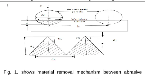
If number of abrasive grains, shape of abrasive and depth of groove are known, we can calculate surface roughness and volume of stock removal. Fig. 1 shows systematic illustration of an abrasive grain and internal workpiece roughness.
The surface roughness value was calculated with the help of mathematical modelling by Jain et al. [16] and was validated with experimental data given by Mittal et al. [18]
Radial force (Fr) or Force of indentation (Fi) can be calculated
by
(12)
dg represents diameter of abrasive grain and σ is the wall
shear value is calculated from FLUENT. And Standard
formula for average diameter of grain (in mm) =
1 . 1
28
eM
Where Me is the Mesh number.
Radial force or force of indentation also written as 2
a
H
A
H
F
F
r
w
w
(13) Hw represents material hardness and a is the radius ofprojected area of indentation ▽A.
The depth of indentation (t) is calculated by
)
(
2
1
2
2 2a
d
d
t
g
g
(14) The shaded portion of the grain (cross sectional area A´ of the
groove generated) shown in the fig.1 can be obtain from the diagram using
4
2 g i rd
F
F
) 2 ( ) ( ) ) ( ( sin 4 2 1 2 t d t d t d t d t d
A g g
g g
g
(15) Volume of material removal is calculated by multiplying cross
sectional area A´ of the groove generated, sum of number of abrasive grain (Ns) for single stroke and length of contact La of
grain with inner surface of workpiece.
s a a
A
L
N
V
(16) Where w a i a a
l
R
R
L
1
0(17)
Rao and Rai represent before and after roughness after ith stroke
and lw is the workpiece length.
And 2 2
2
w m s a w sR
R
L
N
R
N
(18)
Volume of material removal is given by
22 0 2 1 2 1 2 2 1 ) 2 ( ) ( ) ) ( ( sin 2 w m s a w w a i a g g g g g a R R L N R L R R t d t d t d t d t d
V
(19) ΔRa (change in roughness) is calculated from Singh et al. [17]
) 2 ( ) ( ) ) ( ( sin 2 2 1 2 1 2 2 2 1 t d t d t d t d t d R R L N R RR g g
g g g w m a a i a i a
a (20)
4
C
OMPUTATIONALS
IMULATION ANDF
LOWD
ISTRIBUTION4.1 Geometry and Mesh
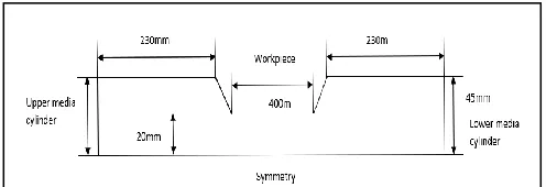
ANSYS FLUENT defined geometry of 2D axisymmetric (symmetrical about axis) model is shown in Fig. 2.
The geometry designed consists of two medium cylinder, fixture and workpiece. The basic function of AFM is to polish surfaces which are difficult to reach therefore tiny abrasive particles (powder form) are assumed as a continuous phase passed through medium cylinders and workpiece having steady state flow regime boundary condition depending upon the rate of change of pressure with time. The meshing of above 2D axisymmetric flow domain model is shown in Fig. 3 is done using ANSYS FLUENT mesh tool. The grid size with no static pressure variation in the flow parameters having
3380 number of cells is taken at individual point in which flow takes place out of four grid sizes having constant value [12].
4.2 SimulationDetails
Multiphase mixture model is used for the simulation of the 2D model in ANSYS FLUENT. The total number of phases selected for mixture model is 2 (phase1 and phase 2). Phase 1 act as primary phase and phase 2 acts secondary phase (continuous phase). The base media consists of natural polymer, silly putty mixed in different proportion with plasticizer. The type of fluid, abrasive particle size and its viscosity is taken from the literature. The viscosity value of media 789 Pa [19] varies depending upon the size of the particle (150µm) [20] and carrier media must behave as Newtonian fluid [21],[12] is selected from literature. The effect of dynamic pressure, strain rate and medium flow velocity is discussed in this paper.
The numerical simulation flow is done using different boundary conditions. The type of model used in Multiphase Mixture model for two phases for primary phase Polyborosiloxane is selected and for Secondary Phase Silicon carbide with operating pressure 101325 Pa [12]. The inlet of workpiece assigned normal pressure to boundary with constant volume fraction for secondary phase, outlet with zero-gauge pressure and wall with no slip boundary conditions.
Analysis assumptions
1. The type of media used must be highly viscous in nature.
2. The media must be made up of parts that are all of same type (uniform properties throughout its volume.) and has the same value when measured in different directions.
3. Properties of media should be temperature independent and value remains constant with respect to space and time.
4. The media flow must be steady state, laminar, symmetric and incompressible about axis for the 2D geometry.
4.3 Validation of model
The results are compared with experimental data extracted Fig. 2. Two-dimensional Axisymmetric geometry taken up for the
simulation
213 from Mittal et al. [18] are listed in Table 1.
TABLE1 DATA USED FOR ANALYSIS
Sr. no. Description Value
1. Workpiece Material Medium Carbon Steel
2.
3.
4.
5.
6.
7.
8.
9.
Material Modulus of elasticity
Diameter of cylindrical workpiece
Length of cylindrical workpiece
Diameter of media Cylinder
Average Length of stroke
Abrasive concentration
Abrasive grain size
Silicon Carbide density
219000 Mpa
20 mm
40 mm
90 mm
230 mm
60%
150
3220 kg/m3
10. Silly putty density 1140 kg/m3
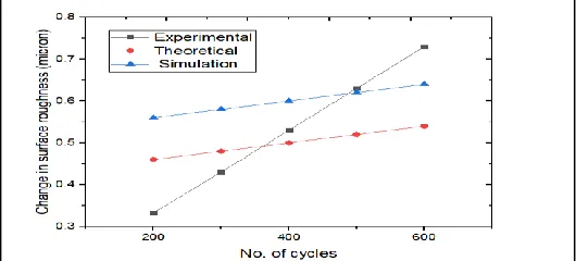
The wall shear value is taken from FLUENT simulation and is calculated to be 13834.591. Shear wall value is used to calculated Radial force from equation 20 and then we can calculate value of t (depth of indentation) using equation (14) and is found to be 3.14576 10-10 m. After solving final
equation, change in surface roughness for single cycle can be calculated using equation (20) and to get value for increasing number of cycles, it is multiplied by the number of cycles and then compared it with experimental, computational and theoretical results. The graph shown in Fig. 4. gives the relation change in roughness (ΔRa) and number of cycles.
5
R
ESULTS ANDD
ISCUSSIONPressure-velocity coupling, momentum and continuity equations, volume of fraction and gradient helps in finding solution results on the basis of different input parameters (controlled parameters). Extrusion pressure, concentration and size of abrasives, velocity of medium flow and media viscosity are the primary parameters which influence AFM process. There are four types of forces acting on an abrasive particle. Normal forces, Tangential force, two resistant forces (wall)and distortion force. Normal forces (vertical driving force) and Tangential forces (horizontal driving force) acting simultaneously and balance each other. Horizontal forces can
be analyzed by pressure and velocity of the abrasive media. The whole pressure acting in the defined geometry depends upon Static pressure and Dynamic pressure. Static and dynamic pressure are important controlled parameters for assessment of tangential forces [22]. Static pressure remains constant and is responsible for media flow varied along the direction of flow of abrasive media whereas Dynamic pressure doesn’t remain same and acts in the direction normal to the flow direction. Experimentally it is difficult to decide the effect of considered response variable therefore few specific parameters on the basis of hypotheses are considered. The considered simulation process parameters used in simulations are defined below in Table 2.
TABLE2 DATA USED FOR ANALYSIS
Sr.no. Parameters Maximum velocity
1 Polyborosiloxane (Primary phase 1) Density- 1219Kg/m3 Viscosity-789 Ns/m2
2 Silicon Carbide (Secondary Phase 2) Density-3170 kg/m3
3
4
5
Abrasive grain Diameter
Velocity at inlet
Secondary phase volume fraction
150µm
0.0068 ms-1,0.0086 ms-1,
0.011 ms-1,0.014 ms-1
0.4
The result from the analysis is discussed on the basis of different contour for dynamic pressure, media flow rate and strain rate for different media flow speed.
Pressure distribution between Static pressure (extend through the direction of flow) and Dynamic pressure (direction normal with the flow direction) is quite different. Static pressure defines the sliding motion and load acting upon the particle. Dynamic pressure defines driving factors for particle rolling and which results to material efficiency decreases with increase in particle rolling [23]. The variation results for Dynamic pressure distribution variation with respect to media flow rate (0.0068 ms-1) shown in Fig. 5 below.
The dynamic pressure value rises with the rise in media flow velocity and secondary phase volume fraction. Maximum value of dynamic pressure (4.18 Pa) indicated by red color and is in the middle of the geometry whose value steadily Fig. 4. Comparison of number of cycles on change in surface
roughness
decreases near the wall and blue color indicates the least pressure. The left side of the bar indicates different values of dynamic pressure in Pascal. The boundary near wall of workpiece surface indicates lower value of dynamic pressure and indicates pressure behavior approaches negligible as a limit from maximum in front of wall area.
Strain rate depends on the force applied, concentration and viscosity of the fluid. The variation of strain rate with respect to media flow speed (0.0068 ms-1) shown in Fig. 6. Due to
friction between adjoining fluid components material removal efficiency and polishing action increases with increases in velocity of different fluid layers and active amount of particles. The strain rate value rises from middle in the direction of the wall and further rises with the value of volume fraction. Red color shows maximum strain value (11.4s-1) which is noticed on the boundary of constriction. Blue
color shows the minimum value for the strain rate. The rate of deformation and wall shear also increases with increase in strain rate. The larger abrasive force in a specific region tends to higher strain rate on the region [24]. For strain rate, concentration of the secondary phase plays important role.
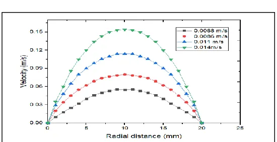
The horizontal flow velocity as well as dynamic pressure play vital part for strengthen particle rolling and remain same [22]. The magnitude of velocity depends upon the secondary phase volume fraction proportionally. The highest velocity value increases with media flow speed. Contour for media flow velocity (0.0068 ms-1) with respect to media flow rate is shown
in above Fig. 7. The maximum value of the media flow velocity is 5.49 10-2 ms-1 and represented by red color.
5.1 Effects of media flow Speed
The effect of different media flow speed on process parameters like dynamic pressure, shear strain and horizontal velocity are described keeping other parameters constant. The graphs show the variation of dynamic pressure, strain rate and velocity with distance from the axis to the wall. In case of Fig. 6. Variation of Strain rate with respect to media flow rate (0.0068
ms-1)
Fig. 7. Variation of Velocity Distribution with respect to media flow rate (0.0068 ms-1)
Fig. 8. Effect of media flow speed with Dynamic pressure vs radial distance from wall
Fig. 9. Effect of media flow speed with Strain rate vs radial distance from wall
215 Dynamic pressure, if we examined the center of passage area
near the specimen surface given in Fig. 5, pressure gradient increases with the rise in media flow velocity. Dynamic pressure is more uniform for volume fraction 0.35 but dynamic pressure at volume fraction 0.8 has more pressure difference and similarly for other parameters. The effect of media flow speed with strain rate vs radial distance from the wall is given in fig. 9. The maximum strain rate value is observed near the wall of specimen surface and narrow passage. The velocity distribution vs radial distance from the wall for different media flow velocity is arranged in the middle of specimen surface. The maximum velocity is in middle and minimum towards the wall and rises with media flow speed per unit time.
6
C
ONCLUSIONAFM process depends upon process parameter like media flow speed, volume fraction etc. The variation of abrasive particle diameter has significant effect on surface finish and MRR. The simulation results in comparison with change in surface roughness (ΔRa) and number of strokes agree better with experimental data. When there is change in volume fraction with respect to media flow speed, there is an increment in dynamic pressure with the rise in inlet velocity value (higher in middle and lower towards the boundary). The strain rate is proportional to media flow speed due to increase in abrasion between adjacent fluid layers. The MRR rises with the rise in wall shear rate. The rate of velocity improves with the rise in media flow rate and further increase gradient and leads to increase in shear stress with increase in MRR. The effect of dynamic pressure and velocity are insignificant near the wall. The results are more defined when extrusion pressure is kept constant and there is change in volume fraction with respect to shear stress, velocity, static pressure and dynamic pressure. But there is non-uniformity increase of pressure, velocity gradient and wall shear with respect to media flow speed. The abrasive particles concentration is more effective in polishing action and abrasive forces apart from media flow rate.
REFERENCES
[1] ―Extrudehoneafm.Com, Accessed 2015/7/10.‖ [2] Y. D. W. Rhoades L.J., Kohut T.A./, Nokovich N.P.,
―Unidirectional abrasive flow machining,‖ Met. Finish., vol. 93, no. 6, p. 155, 1995, doi: 10.1016/0026-0576(95)94768-x.
[3] L. J. Rhoades and T. A. Kohut, ―Reversible Unidirectional AFM,‖ 1991.
[4] R. Lawrence J., ―Orbital and/or Reciprocal Machining with a Viscous Plastic Medium,‖ 1990.
[5] I. T. Im, S. D. Mun, and S. M. Oh, ―Micro machining of an STS 304 bar by magnetic abrasive finishing,‖ J. Mech. Sci. Technol., vol. 23, no. 7, pp. 1982–1988, 2009, doi: 10.1007/s12206-009-0524-z.
[6] V. K. Gorana . V. K. Jain . G. K. Lal, ―Prediction of surface roughness during abrasive flow machining,
Int J Adv Manuf Technol.‖
[7] J. W. E.Uhlmann, C.Schmicdel, ―CFD simulation of the abrasiv flow machining process,‖ pp. 207–214, 2015.
[8] R. Butola, R. Jain, P. Bhangadia, A. Bandhu, R. S. Walia, and Q. Murtaza, ―Optimization to the parameters of abrasive flow machining by Taguchi method,‖ Mater. Today Proc., vol. 5, no. 2, pp. 4720– 4729, 2018, doi: 10.1016/j.matpr.2017.12.044.
[9] P. Ali, S. Dhull, R. S. Walia, Q. Murtaza, and M. Tyagi, ―ScienceDirect Hybrid Abrasive Flow Machining for Nano Finishing - A Review,‖ Mater. Today Proc., vol. 4, no. 8, pp. 7208–7218, 2017, doi: 10.1016/j.matpr.2017.07.048.
[10]V.K.Jain and S.G.Adsul, ―Experimental investigations into abrasive flow machining (AFM), International Journal of Machine Tools & Manufacture,.‖
[11]G. Venkatesh, A. K. Sharma, N. Singh, and P. Kumar, ―Finishing of bevel gears using abrasive flow machining,‖ Procedia Eng., vol. 97, pp. 320–328, 2014, doi: 10.1016/j.proeng.2014.12.255.
[12]P. Pal and K. K. Jain, ―Computational Simulation of Abrasive Flow Machining for Two Dimensional Models,‖ Mater. Today Proc., vol. 5, no. 5, pp. 12969– 12983, 2018, doi: 10.1016/j.matpr.2018.02.282.
[13]R. S. Mulik and P. M. Pandey, ―Experimental investigations and modeling of finishing force and torque in ultrasonic assisted magnetic abrasive finishing,‖ J. Manuf. Sci. Eng. Trans. ASME, vol. 134, no. 5, pp. 1–9, 2012, doi: 10.1115/1.4007131.
[14]R. K. Singh, D. K. Singh, and S. Gangwar, ―Advances in Magnetic Abrasive Finishing for Futuristic Requirements - A Review,‖ Mater. Today Proc., vol. 5, no. 9, pp. 20455–20463, 2018, doi: 10.1016/j.matpr.2018.06.422.
[15]M. Syamlal, W. Rogers, and T. . O’Brien, ―MFIX Documentation,‖ Natl. Tech. Inf. Serv., vol. 1, 1993, doi: METC-9411004, NTIS/DE9400087.
[16]R. K. Jain, V. K. Jain, and P. M. Dixit, ―Modeling of material removal and surface roughness in abrasive flow machining process,‖ Int. J. Mach. Tools Manuf., vol. 39, no. 12, pp. 1903–1923, 1999, doi: 10.1016/S0890-6955(99)00038-3.
[17]S. Singh, M. R. Sankar, V. K. Jain, J. Ramkumar, M. Engineering, and I. I. T. Guwahati, ―Modeling of Finishing Forces and Surface Roughness in Abrasive Flow Finishing ( AFF ) Process using Rheological Properties,‖ no. Aimtdr, pp. 2–7, 2014.
[18]M. Sushil, K. Vinod, and K. Harmesh, ―Multi-objective optimization of process parameters involved in micro-finishing of Al/SiC MMCs by abrasive flow machining process,‖ Proc. Inst. Mech. Eng. Part L J. Mater. Des. Appl., vol. 232, no. 4, pp. 319–332, 2018, doi: 10.1177/1464420715627292.
815–820, 2009, doi: 10.1109/CAIDCD.2009.5374887. [20]V. K. Jain and S. G. Adsul, ―Experimental
investigations into abrasive flow machining (AFM),‖ Int. J. Mach. Tools Manuf., vol. 40, no. 7, pp. 1003– 1021, 2000, doi: 10.1016/S0890-6955(99)00114-5. [21]R. K. Jain, V. K. Jain, and P. K. Kalra, ―Modelling of
abrasive flow machining process: A neural network approach,‖ Wear, vol. 231, no. 2, pp. 242–248, 1999, doi: 10.1016/S0043-1648(99)00129-5.
[22]R. S. Walia, H. S. Shan, and P. Kumar, ―Enhancing AFM process productivity through improved fixturing,‖ Int. J. Adv. Manuf. Technol., vol. 44, no. 7– 8, pp. 700–709, 2009, doi: 10.1007/s00170-008-1893-7. [23]K. T. Subramanian, N. Balashanmugam, and P. V.
Shashi Kumar, ―Nanometric Finishing on Biomedical Implants by Abrasive Flow Finishing,‖ J. Inst. Eng. Ser. C, vol. 97, no. 1, pp. 55–61, 2016, doi: 10.1007/s40032-015-0190-0.