City, University of London Institutional Repository
Citation
:
Vogiatzaki, K., Navarro-Martinez, S., De, S. and Kronenburg, A. (2015). Mixing
modelling framework based on Multiple Mapping Conditioning for the prediction of turbulent
flame extinction. Flow, Turbulence and Combustion, 95(2), pp. 501-517. doi:
10.1007/s10494-015-9626-0
This is the accepted version of the paper.
This version of the publication may differ from the final published
version.
Permanent repository link:
http://openaccess.city.ac.uk/8130/
Link to published version
:
http://dx.doi.org/10.1007/s10494-015-9626-0
Copyright and reuse:
City Research Online aims to make research
outputs of City, University of London available to a wider audience.
Copyright and Moral Rights remain with the author(s) and/or copyright
holders. URLs from City Research Online may be freely distributed and
linked to.
City Research Online:
http://openaccess.city.ac.uk/
[email protected]
UNCORRECTED
PR
OOF
Mixing Modelling Framework Based on Multiple
Mapping Conditioning for the Prediction of Turbulent
Flame Extinction
1 2 3
K. Vogiatzaki1·S. Navarro-Martinez2·S. De3· A. Kronenburg3
4 5
Received: 5 January 2015 / Accepted: 6 June 2015 6 © Springer Science+Business Media Dordrecht 2015 7
Abstract A stochastic implementation of the Multiple Mapping Conditioning (MMC) 8
approach has been applied to a turbulent piloted jet diffusion flame (Sandia flame F) that 9
is close to extinction. Two classic mixing models (Curl’s and IEM) are introduced in the 10
MMC context to model the turbulent mixing. The suggested model involves the use of a 11
reference space (that is mapped to mixture fraction space) in order to define particle prox- 12
imity. The addition of the MMC ideas to the IEM and Curl’s models, that is suggested in 13
the current work, aspires to combine the simplicity of these two models with the enforced 14
compositional locality without violating the linearity and independence principles. The for- 15
mulation of the approach is discussed in detail and results are presented for the mixing field 16
and reactive species. The predictions are compared with joint-scalar PDF simulations using 17
the same mixing models and experimental data. Moreover, the sensitivity of the model to 18
the particle number is examined. It is shown that MMC is less sensitive to the number of 19
particles and can generally produce improved predictions of major and minor chemically 20
reacting species with a lower number of particles. 21
K. Vogiatzaki
[email protected] S. Navarro-Martinez
[email protected] S. De
[email protected] A. Kronenburg
UNCORRECTED
PR
OOF
Keywords Multiple mapping conditioning·Mixing models·Probability density function
22
approach·Sandia flame F
23
1 Introduction
24
An important safety issue for engineers of combustion systems is the appearance of local
25
extinction and re-ignition of the flame. These phenomena can be directly linked to the levels
26
of turbulence in the combustion chamber. Overall, turbulence is a physical process highly
27
desirable in combustion devices since it enhances the mixing of the fuel and oxidiser and
28
accelerates the combustion process. However, due to its chaotic nature, small changes can
29
result in a considerable increase of its intensity. If a critical value is exceeded very small
30
eddies are generated that can penetrate the reaction zone reducing the flame temperature
31
and disrupting the formation of radicals. Under these conditions the chemistry deviates
32
from equilibrium and regions on the stoichiometric surface begin to extinguish. This could
33
lead to global flame extinction or the flame may re-ignite depending on local strain-rate
34
conditions.
35
Direct Numerical Simulation (DNS) would be the only numerical method capable of
pro-36
viding a detailed description of extinction and re-ignition since burning and mixing occurs
37
mostly at the smallest scales. However, due to the very large computing requirements
Large-38
eddy (LES) and Reynolds averaged (RANS) simulations are the two alternative methods
39
commonly used that involve some extra modelling. Although LES has drawn considerable
40
attention of the academic community over the last decade, its application has not yet quite
41
reached the industry sector. On the other hand RANS based CFD codes are still widely used
42
in industries. In both, the RANS and LES contexts the instantaneous scalar dissipation –the
43
term used to describe the levels of the mixing rate– is unclosed and thus the research around
44
new turbulence combustion approaches that represent more accurately the mixing process
45
is still very important.
46
The objective of the present work is to ascertain the capability of the Multiple
Map-47
ping Conditioning (MMC) approach [21] and its closures to capture local extinction and
48
re-ignition in laboratory flames in the RANS context. The MMC framework combines the
49
probability density function (PDF) approach [27] and the mixture fraction based methods
50
[20] via the application of a generalised mapping function to a prescribed reference space.
51
PDF methods have been extensively applied to the modelling of turbulent reacting flows and
52
a relatively recent comprehensive review is given by Haworth [14]. Of particular relevance
53
are the studies by Pope and co-workers [3,4,36] where sensitivities of the PDF modelling
54
approach towards parameters such as the mixing model [4], the mixing time scale [4] and
55
the chemical mechanism [3] were investigated. Raman and Pitsch [30] successfully adapted
56
the PDF methods as sub-grid scale model for large-eddy simulations. The Sandia flame
57
series with flames of moderate to significant local flame extinction (Sandia Flames E and
58
F) [1,2] served as a test bed for all these modelling validation studies, and the same flames
59
are used here for the validation of the MMC models.
60
With respect to the MMC modelling, stochastic and deterministic formulations exist, and
61
both formulations have been explored in the past for the simple case of Sandia flame D [32,
62
33], a flame with a relatively low degree of extinction. Variants of the original MMC
for-63
mulation have been successfully applied to Sandia Flame E (and Flame F) using a hybdrid
64
binomial Langevin-MMC model for the modelling of the velocity-scalar interactions [35] or
65
using a sparse particle method as sub-grid model for LES of the turbulent flow and mixing
66
fields [12,13]. In this work we focus exclusively on the stochastic implementation in the
UNCORRECTED
PR
OOF
RANS context, we base the MMC mixing model on the IEM and Curl’s models (as opposed 68
to IEM only that was used in earlier work [33]), we expand our study to the more challenging 69
case of Sandia flame F, a flame with a relatively high Reynolds number and a considerable 70
degree of extinction and re-ignition that has never been explored in the MMC context, and 71
we assess the model dependence on the number of particles used for the stochastic solution 72
of the composition field. 73
2 Turbulence-Chemistry Interaction Model
742.1 The PDF approach 75
Conventional PDF methods are based on the solution of the following equation that 76
describes the evolution of the joint (one point) scalar PDFP = P (y,x, t)of a set ofns 77
scalarsYI (I=1, .., ns). 78
∂ρPY
∂t + ∇(ρuYPY)+
∂ρ|yPY
∂yi +
∂2ρNI JPY
∂yi∂yj =
0, (1)
whereuY is the conditional expectation of the flow velocity v(uY(y,x, t)= v|Y = y) 79
andNI J is the conditional scalar dissipation,NI J = D∇YI∇YJ|Y = y, which is by 80
definition symmetric and positive semidefinite. The termDis the diffusion coefficientDI J 81
(which is assumed to be the same for all species in high Reynolds number flows) andI is 82
the reaction rate. 83
The most commonly adopted approach to solving the above PDF evolution equation is 84
the Lagrangian stochastic particle method, where the evolution of an ensemble of particles 85
is used to represent the evolution of the (Eulerian) joint PDF of Eq.1. In terms of imple- 86
mentation of the framework, a Lagrangian solver for the composition joint PDF is coupled 87
with a standard Eulerian approach [14,24,25]. The solution domain in physical space is 88
discretized into a number of cells for the purpose of extracting local mean quantities such as 89
velocities which are then used in the particle evolution equations. Then, moments of reac- 90
tive species, temperature and mixture fraction can be extracted by ensemble (or weighted) 91
average of the particles in the same Eulerian cell. Properties of particles drawn from the 92
same cell are considered to be local in the physical space. This approach is followed in the 93
current work as well. Equation1is replaced by an equivalent set of stochastic differential 94
equations of the following form 95
dx∗=(v(x∗,t)+ 1 ρ
∂
∂x(ρ(D+Dt)))dt+
2(D+Dt)dw∗i, (2)
96
dYI∗= [∗I +SI∗]dt. (3) The underlying idea is that the Fokker-Planck equation [11] that corresponds to the above 97
set of equations has the same moments as those given by the PDF transport Eq. 1. Here 98
and for the remainder of the paper, the superscript ’*’ is used to distinguish the values 99
linked to stochastic trajectories (stochastic particles), from deterministic quantities, Dt is 100
the turbulent diffusivity and approximated byDt ≈0.09∗k2//σtwithσt =0.7 being the 101
turbulent Schmidt number. Equation 2accounts for transport in physical space while Eq.3 102
accounts for transport in the composition space. The location of the particles is indicated 103
asx∗,w∗i is a Wiener process with zero mean and variance equal todt andS∗is a mixing 104
operator that simulates the rate of change of scalar dissipation and in the Lagrangian particle 105
UNCORRECTED
PR
OOF
particle under the effect of molecular mixing. The v(x∗, t)term is calculated by using the
107
mean Eulerian velocity field v(x, t)interpolated to the particle positionx∗.
108
For the modelling ofS∗certain principles should be satisfied by the mixing models such
109
as boundedness of the scalars, linearity of scalar transport, independence of the evolution
110
of the particle properties and most importantly localness in the physical and compositional
111
spaces [27,31]. Treating fluid as continuum, molecular diffusion is an exchange of
composi-112
tion between neighboring fluid particles which are infinitesimally close in both position and
113
in composition. Although localness in the physical space is easy to impose in most models
114
by allowing ”mixing” among particles that belong to the same cell, localness in composition
115
space is a major problem and much more difficult to impose [26]. Results [31] suggest that
116
if particles mix with other particles in their immediate neighbourhood in composition space
117
so that mixing across the reaction zone is avoided, the description of mixing is improved.
118
On the contrary ”artificial” extinction can be predicted for turbulent non-premixed flames
119
at infinite Damk¨oler number if the principle of localness in composition space is violated.
120
An additional difficulty is that in reality localness in the physical space and localness in the
121
composition space in particle methods are two principles that interlink. In a recent study by
122
[19] it is demonstrated that closeness in physical space can be related –in addition to
local-123
ness in composition space– to the number of particles used in the calculations and of course
124
to the resolution limitations originating from the resolution of the underlying Eulerian flow
125
fields.
126
Different models have been suggested in the literature forS∗. Simple models that are
127
easy to implement, such as the interaction by exchange with the mean (IEM) [10] and the
128
various Curl’s models [9,16] do not ensure localness in the composition space. A more
129
recent model, the Euclidean minimum spanning tree (EMST) [31] enforces locality but
130
implementation is rather complicated, and it violates the linearity and independence
princi-131
ples. A promising new model the shadow-position mixing model (SPMM), was introduced
132
in 2013 in [29] however up to date its applicability has only been demonstrated for the
ide-133
alised case of a reactive scalar mixing layer. The addition of the MMC ideas to the IEM and
134
Curl’s model that is suggested in the current work and described in detail in the next
sec-135
tion, aspires to combine the simplicity of these two models with the enforced compositional
136
locality without violating the linearity and independence principles.
137
2.2 The MMC concept
138
MMC, by the use of a reference space, addresses some of the problems described in the
139
previous section associated with the modelling of the mixing term. The basic idea of the
140
mapping closure concept [5,28] is to employ turbulent fluctuations and small-scale mixing
141
in a mathematical reference space,ξ, with a known (or prescribed) PDF to model the mixing
142
in the physical composition space with unknown PDF. A deterministic implementation of
143
the method leads to closure of the conditional scalar dissipation [7,17]. In the present
144
paper, we focus on a stochastic implementation. If the reference space is chosen properly it
145
can be used to enforce localness in composition space [21,34]. The idea is to track particle
146
position in the reference space and then allow mixing only among particles that are close to
147
each other inξ-space. Theoretically, events close in physical space should also be close in
148
composition space, ensuring the localness of the MMC model.
149
The suggested approach can considered to be an extension to the work of Wandel et
150
al. [34] and has already been applied for the case of Sandia flame D using IEM as the only
151
underlying mixing model [33]. It is a probabilistic MMC formulation with a single reference
152
variable that is used to enforce localness in mixture fraction space and whose evolution
UNCORRECTED
PR
OOF
is described by a Markov process. MMC allows the choice of any number of reference 154
variables, yet for flames with low levels of local extinction, localness in mixture fraction 155
space is known to be sufficient to indicate localness in the multidimensional composition 156
space. In a broader sense the shadow position model of [29] can be seen as a variation 157
of the MMC concept where instead of enforcing locality through mixture fraction space, 158
mixing is modeled as a relaxation of the composition to its mean conditional on the shadow 159
position. In the present work we test if the enforced locality imposed by MMC can capture 160
the behaviour of flames close to blow off. 161
We introduce a stochastic reference variable,ξ∗, which is governed by the following set 162
of sdes 163
dx∗=U (ξ∗)dt, (4)
164
dξ∗=Aodt+bodw∗ (5)
and for which we assume that the distribution is known. 165
The Fokker-Planck equation representing the above sde can be written as 166
∂Pξ
∂t + ∇UPξ+ ∂AoPξ
∂ξ − ∂2BoPξ
∂ξ2 =0, (6)
where 2Bo=(bo)2. Considering an arbitrary function ofξ∗,f (ξ∗)=f∗a corresponding 167
sde for this new random variable can be generated using an Ito transformation: 168
df (ξ∗)=Adt +bdw∗, (7)
with 169
A=∂f (ξ )
∂t +U∇f (ξ )+
Ao∂f (ξ ) ∂ξ +B
o∂2f (ξ )
∂ξ2
(8)
and 170
b=bo∂f (ξ )
∂ξ (9)
The Fokker Planck equation representing the above sde is given by 171
∂Pf
∂t + ∇U Pf+ ∂AP f
∂f − ∂2BP f
∂f2 =0. (10)
The advantage of the “mapping ” is that by assuming a shape forPξwe can defineAoand 172
bofrom Eq.6. We can then define the unknown drift and diffusion coefficients for the new 173
stochastic processf (ξ∗)and consequently the evolution of its PDF. It should be noted that 174
the equivalent PDF describes the one-point one-time cell distribution. A two-point strategy 175
has been suggested based on mapping functions that incorporate two-points statistics [15] 176
however it has not been attempted here. 177
Following the probabilistic approach and adding to the equations for a standard PDF 178
approach, Eqs.2and3, the two new MMC equations, Eqs.5and7, that embody the mapping 179
closure concept, the general probabilistic approach gives 180
dx∗=U (ξ∗)dt, (11)
181
dξ∗=Aodt+bodw∗, (12) 182 dY (ξ∗)=Adt +bdw∗, (13) 183
dY∗= [∗I +SI∗]dt. (14) It should be noticed that Eq.13is not solved since it is in reality equivalent to Eq.12. 184
This mathematical equivalence is the key that explaines the concept that an appropriate 185
UNCORRECTED
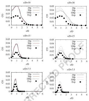
PR
OOF
the computational cost low, the reference variables generate the fluctuations of a selected
187
number of species only (the so called “major species”) and the fluctuations of the remaining
188
species (the so called “minor species”) are linked to the fluctuations of major species similar
189
to the conditional moment closure methodology [21]. Thus, it is only necessary to establish
190
mapping relations as Eq.13for the major species and this is here mixture fraction,Z. For
191
each major species that has a corresponding reference variable, the MMC transport equation
192
becomes a PDF transport equation [21], [18]. Thus,Ao,BoandU (ξ∗)must be chosen so
193
thatAandBdescribe a diffusion process for mixture fraction. If we assume a Gaussian
194
distribution for the reference variable and equate Eqs.10to1for mixture fraction we can
195
obtain the unknown coefficientAoandbofrom
196
U=U(ξ;x, t)=U(0)+U(1)ξ, (15)
197
Ao= −∂B
o
∂ξ +B
oξ+ 1
ρ∇ρU
(1)+ 2
Pξ
∂BoPξ
∂ξ , (16)
198
U(0)= v, (17)
199
U(1)ξ Z = vZ. (18) The turbulent flux can be modelled by a standard gradient approximation, vZ =
200
−Dt∇ < Z >andξ Zresults directly from the solution ofZ(ξ )(c.f Fig.1). The term
201
Bois modelled independently ofξ,Bo =Bo(x, t)), and is related to the scalar dissipation
202
NZthrough
203
Bo
∂Z ∂ξ
2
= NZ. (19)
It is apparent from Eq.19that closure of the MMC model requires knowledge of the
204
unconditional scalar dissipation ofZ, but it does not explicitly include the more difficult
205
to model conditional scalar dissipation. The dissipationNZcan be modelled adopting
206
Corrsin’s suggestion [8] that the decay rate of a passive scalar variance is assumed to be
207
proportional to the decay rate of the turbulent kinetic energy i.e.
208
NZ =0.5
Z2 τD
, (20)
whereτD is proportional to the flow turbulent time scaleτ = k/εwith a proportionality
209
constant commonly assumed to beCD=1/Cφ =0.5.
210
It should be noted that three different definitions of fluctuations exist in MMC: the
211
unconditional fluctuations or major fluctuationsYI = YI − YI, the minor fluctuations
212
YI=YI−YI|ξand the fluctuations around a quantity, conditionally averaged on mixture
213
fraction itself,YI = YI − YI|Z. The diffusion coefficientBo controls the major
fluc-214
tuations while the mixing operatorSI∗controls the minor fluctuations. In the current work
215
two different models have been implemented which are essentially modified versions of the
216
well known IEM and Curl’s model.
217
When using the modified IEM model (MMC-IEM) the particles are mixed with their
218
means conditioned on a certain value in the reference spaceYI|ξ
219
SI∗= 1 2
YI(ξ∗)−YI∗p
τmin
. (21)
For the modified version of the Curl’s model (MMC-Curl’s) at each time step all particles
220
that belong to the same Eulerian cell are formed into pairs and mix with their mean. The
221
selection of every particle pair is not random as in commonly used Curl’s models but it is
UNCORRECTED
PR
OOF
according to the distance of the particles in the reference space. For the present work, only 223
particles that belong to the sameξ-bin are allowed to mix following 224
S∗I = 1 2
0.5(YI∗p+YI∗q)−YI∗p τmin
, (22)
with< S∗|ξ∗, x∗>= 0 [21]. The simplicity of both models is attractive for implementa- 225
tion, but the estimation of the “minor dissipation time”,τmin, is rather problematic since 226
minor fluctuations exist only in the context of MMC. Wandel and Klimenko [34] used DNS 227
of homogeneous turbulence to obtain a time scale ratio between the minor and major dissi- 228
pation time ofτmin/τD=1/8. However, Vogiatzaki et al. [33] could not corroborate these 229
findings for laboratory jet diffusion flames. Mixing time scales smaller thanτDwere found 230
to suppress most minor fluctuations and lead to a significant underprediction of the condi- 231
tionally averaged variances. For Sandia Flame D, best results were obtained withτmin =τD, 232
and this value is adopted here. 233
3 Computational Methods
234The test case (Sandia flame F) [1] consists of a methane/air fuel mixture that issues from a 235
central d= 7.2mm internal diameter nozzle surrounded by a coaxial pilot flame with an outer 236
diameter of 18.2mm. The fuel is 25 %CH4and 75 % air by volume with a stoichiometric 237
mixture fraction ofZst=0.351. The jet Reynolds number is 44,800, the pilot inlet velocity 238
is 22.8m/sand the velocity of the co-flowing air is 0.9m/s. 239
The PDF approach is used in order to model the turbulence-chemistry interaction. The 240
composition PDFs are calculated by Monte Carlo methods, while a finite-volume method 241
was applied to solve for the mean velocity, dissipation, and mean pressure fields. The Eule- 242
rian flow field equations are solved using an in-house RANS code (BOFFIN). Turbulence 243
is modelled by a standardk-εmodel [23]. A cylindrical domain extends 0.65min down- 244
stream direction and 0.15min radial direction and is discretised by 200 axial and 100 radial 245
finite volume cells. An augmented reduced mechanism (ARM2) derived from the full GRI 246
3.0 mechanism using quasi-steady assumptions for some minor species is incorporated to 247
describe the chemical reactions [6]. Cao and Pope [3] demonstrated that ARM2 is capa- 248
ble of predicting the correct extinction levels for all Sandia Flames D-F but for flame F, 249
results may be sensitive towards small changes in the boundary conditions or modelling 250
parameters. For the composition field calculations, three different particle densities have 251
been used in order to asses the sensitivity of the models on particle number. The differ- 252
ent test cases are listed in Table 1. The evolution of the particle properties is modelled 253
by Eqs. 11 to14. We emphasise that every particle carries information on its (stochas- 254
tic) velocity, species concentration, temperature and reference space ξ, obtained from 255
Eq.12. 256
Note that the reference space is Gaussian and unbounded, but the deterministic drift 257
[image:8.440.168.394.555.616.2]term counteracts the random diffusion term and keeps particles close to the mean. Then 258
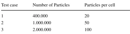
Table 1 Overview of the test
cases with corresponding number of particles
Test case Number of Particles Particles per cell
1 400.000 20
2 1.000.000 50
UNCORRECTED
PR
OOF
depending on theirξvalue the particles within each cell are ordered in the reference sample
259
space that extends from -4 to 4, divided into 16ξ-bins. In eachξ-bin,YI|ξis defined by an
260
ordinary averaging process. For emptyξ-bins, values are obtained from linear interpolation.
261
It is important to emphasize that the calculations with 20 particles/cell take 5 hours on
262
a single core machine. The computational cost is tripled when the number of particles is
263
increased to 100 particles per cell. Previous Lagrangian PDF approaches in the RANS
con-264
text use a wide range of particle numbers (from 100 particles/cell [36] to 800 particles/cell
265
[24]). Although the absolute computational time depends on the specific characteristic of
266
the codes used in these calculations, it is obvious that a significant increase of the
num-267
ber of particles will significantly increase the computational cost. This increase can be very
268
important for the calculation of a realistic industrial geometry with a considerably bigger
269
grid. Thus, a very desirable characteristic of any new mixing model is to perform well with a
270
relatively low number of particles per cells. This motivated the three numerical experiments
271
with different numbers of particles
272
4 Results and Discussion
273
Figure1is a graphic representation of the MMC concept at x/d =15 at three radial locations
274
of the flame under consideration: on the rich side (r/d = 0.1 ), in the shear layer (r/d =1)
275
and on the lean side (r/d = 2). As mentioned above every particle carries a set of values that
276
represent its (stochastic) velocity, species concentration, temperatureandξ. This creates a
277
correlation between temperature, (or any reactive species), mixture fraction and reference
278
T
r/d=0.1 r/d=1 r/d=2
T
Z
0 0.2 0.4 0.6 0.8 1 0.2 0.4 0.6 0.8 0 0.2 0.4 0.6 0.8 1 -4 -2 0 2 4
-4 -2 0 2 4 -4 -2 0 2 4 -4 -2 0 2 4 -3 -2 -1 0 1 2 3
-3 -2 -1 0 1 2 3
1
0.8
0.6
0.4 0.2 0 2500
2000
1500
1000
500
2500
2000
1500
1000
5000
Fig. 1 MMC mapping concept: first row – temperature versus reference space at three radial locations; second row – computed mapping function; third row – temperature versus mixture fraction for the MMC-IEM
UNCORRECTED
PR
OOF
space which is demonstrated in the top two rows of the figure. Closeness of the particles 279
in the reference space controls closeness of the particles in the mixture fraction fraction 280
space and consequently in the temperature (or composition) space as can be seen in the 281
figures in the bottom row. This correlation exists only because the evolution of the reference 282
space, Eq. 12, is not independent of the evolution of the species, Eq.13. Consequently, 283
mixing particles that are close in reference space is equivalent to mixing particles close in 284
composition space. It is important to stress that if the particle’s value of the reference space 285
was held constant throughout the calculations, the reference variable and mixture fraction 286
would decorrelate with time (or distance from the jet exit) and the method would collapse 287
to a conventional PDF approach. The decorrelation would be equivalent to horizontal lines 288
of the averaged mixture fraction,Z|ξ, in the middle row of Fig.1. 289
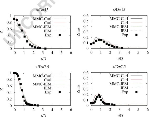
In Fig.2the radial profiles of the mean and root mean square (rms) of the mapping func- 290
tion (mixture fraction) are presented for all four mixing models, IEM, MMC-IEM, Curl’s 291
and MMC-Curl’s. It is apparent that the mixing field is quite insensitive to the choice of the 292
mixing model. The simulations presented in this figure are performed with 20 particles/cell, 293
the quality of predictions for test cases 1 to 3 (see Table1) is comparable for all models and 294
none of them shows a significant dependence on the particle number. As it has been shown 295
in previous studies [4,36] the predictions for the mixture fraction depend mostly on the 296
[image:10.440.80.363.374.597.2]choice of the mixing time scale that for the current work is the same for all four models. 297
Figures3,4,5and6show the scatter plots of temperature at different axial locations 298
for three different particle loadings. Figure 7 shows the experimental results and serves 299
as comparison. These figures allow a qualitative assessment, and MMC (both with IEM 300
and Curl’s), yields a somewhat more realistic scatter in temperature with fewer realizations 301
above equilibrium conditions than the classic models. The MMC-IEM model is not capa- 302
ble of fully capturing the extent of extinguished flame elements as seen in the experiments, 303
but it needs to be emphasized here that MMC-IEM provides qualitatively reasonable pre- 304
dictions even with a very small number of particles. These results should be compared with 305
0 0.1 0.2 0.3 0.4 0.5 0.6
0 1 2 3 4 5 6
Zrms
r/D x/D=7.5 MMC-Curl
Curl MMC-IEM IEM Exp 0
0.1 0.2 0.3 0.4 0.5 0.6
0 1 2 3 4 5 6
Zrms
r/D x/D=15 MMC-Curl
Curl MMC-IEM IEM Exp
0 0.2 0.4 0.6 0.8 1
0 1 2 3 4 5 6
Z
r/D x/D=7.5 MMC-Curl
Curl MMC-IEM IEM Exp 0
0.2 0.4 0.6 0.8 1
0 1 2 3 4 5 6
Z
r/D x/D=15 MMC-Curl
Curl MMC-IEM IEM Exp
UNCORRECTED
PR
OOF
500 1000 1500 2000 25000 0.2 0.4 0.6 0.8 1
T
Z x/d = 7.5
20p 500 1000 1500 2000 2500
0 0.2 0.4 0.6 0.8 1
T
Z x/d = 15
20p 500 1000 1500 2000 2500
0 0.2 0.4 0.6 0.8 1
T
Z x/d = 7.5
50 500 1000 1500 2000 2500
0 0.2 0.4 0.6 0.8 1
T
Z x/d = 15
50 500 1000 1500 2000 2500
0 0.2 0.4 0.6 0.8 1
T
Z x/d = 7.5
100 500 1000 1500 2000 2500
0 0.2 0.4 0.6 0.8 1 Z x/d = 15
100
Fig. 3 MMC-IEM: scatter plots of temperature at different axial locations and for different particle number
densities
conventional IEM simulations (see Fig.4). The IEM mixing model creates two very
dis-306
tinct branches, one burning and one non-burning, that are not present in Fig.7and yield an
307
unphysical bias towards certain realizations in composition space. Note that the
computa-308
tion of the mean value in the cell, used for the mixing model, is based on the instantaneous
309
cell population and it slightly varies with the iteration and is thus dependent on the number
310 500 1000 1500 2000 2500
0 0.2 0.4 0.6 0.8 1
T
Z x/d = 7.5
20p 500 1000 1500 2000 2500
0 0.2 0.4 0.6 0.8 1
T
Z x/d = 15
20p 500 1000 1500 2000 2500
0 0.2 0.4 0.6 0.8 1
T
Z x/d = 7.5
50p 500 1000 1500 2000 2500
0 0.2 0.4 0.6 0.8 1 Z x/d = 15
50p 500 1000 1500 2000 2500
0 0.2 0.4 0.6 0.8 1
T
Z x/d = 7.5
100p 500 1000 1500 2000 2500
0 0.2 0.4 0.6 0.8 1 Z x/d = 15
[image:11.440.68.373.55.259.2]100p
Fig. 4 IEM: Scatter plots of temperature at different axial locations and for different particle number
[image:11.440.76.361.374.589.2]UNCORRECTED
PR
OOF
500 1000 1500 2000 25000 0.2 0.4 0.6 0.8 1
T
Z x/d = 7.5
20p 500 1000 1500 2000 2500
0 0.2 0.4 0.6 0.8 1
T
Z x/d = 15
20p 500 1000 1500 2000 2500
0 0.2 0.4 0.6 0.8 1 Z x/d = 7.5
50p 500 1000 1500 2000 2500
0 0.2 0.4 0.6 0.8 1 Z x/d = 15
50p 500 1000 1500 2000 2500
0 0.2 0.4 0.6 0.8 1 Z x/d = 7.5
100p 500 1000 1500 2000 2500
0 0.2 0.4 0.6 0.8 1 Z x/d = 15
100p
Fig. 5 MMC-Curl’s: Scatter plots of temperature at different axial locations and for different particle number
densities
of the particles in the cell. The dependence of the IEM model on particle number would 311
vanish if averages over many iteration would be used instead. 312
The MMC-Curl’s model appears to provide the best qualitative agreement with the exper- 313
imental data especially further downstream. The conventional Curl’s model also predicts 314
the extinction satisfactorily, but some spurious behaviour can be observed especially on the 315
lean side when only few particles are used. The reader should note that we have used the 316
500 1000 1500 2000 2500
0 0.2 0.4 0.6 0.8 1
T
Z x/d = 7.5
20p 500 1000 1500 2000 2500
0 0.2 0.4 0.6 0.8 1
T
Z x/d = 15
20p 500 1000 1500 2000 2500
0 0.2 0.4 0.6 0.8 1
T
Z x/d = 7.5
50 500 1000 1500 2000 2500
0 0.2 0.4 0.6 0.8 1 Z x/d = 15
50 500 1000 1500 2000 2500
0 0.2 0.4 0.6 0.8 1
T
Z x/d = 7.5
100 500 1000 1500 2000 2500
0 0.2 0.4 0.6 0.8 1 Z x/d = 15
[image:12.440.72.374.54.262.2]100
Fig. 6 Curl’s: Scatter plots of temperature at different axial locations and for different particle number
[image:12.440.76.363.382.588.2]UNCORRECTED
PR
OOF
500 1000 1500 2000 2500
0 0.2 0.4 0.6 0.8 1
T
Z x/d = 7.5
Exp
500 1000 1500 2000 2500
0 0.2 0.4 0.6 0.8 1
T
Z x/d = 15
[image:13.440.76.363.59.160.2]Exp
Fig. 7 Experiment: Scatter plots of temperature at different axial locations
simple Curl’s model in its original form and not its modified version. No additional control
317
of the mixing process to limit unphysical super-equilibrium values has been attempted.
318
A better insight is provided by Figs.8and9. Here, the radial profiles of the conditional
319
temperature and its conditional rms at different axial locations are presented and the
MMC-320
IEM and IEM models can be compared. It can be clearly seen that IEM shows a strong
321
dependence on the particle number while MMC-IEM is much less sensitive to particle
den-322
sity and only 20 particles per cell yield an independence of the solution from the particle
323
density while IEM requires around 100 particles/cell to approximate the same results. The
324
conditional rms are considerably under-predicted for the MMC-IEM and the IEM model
325
appears to be somewhat better. However these predictions should be always viewed in
con-326
junction with Figs.3and4. The high rms values result from unphysical mixing of particles
327
that create two distinct burning modes rather than a uniform scattering as the one seen in
328
the experiments (see Fig.7).
329
These trends are similar but much less pronounced for MMC-Curl’s and Curl’s model
330
(not shown here). MMC-Curl’s and Curl’s yield conditional temperatures closer to the
331
experimental values at both axial locations, and the classic Curl’s mixing model is only
332
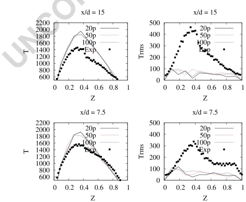
0 100 200 300 400 500
0 0.2 0.4 0.6 0.8 1
Trms
Z x/d = 7.5
20p 50p 100p Exp 0
100 200 300 400 500
0 0.2 0.4 0.6 0.8 1
Trms
Z x/d = 15
20p 50p 100p Exp
600 800 1000 1200 1400 1600 1800 2000 2200
0 0.2 0.4 0.6 0.8 1
T
Z x/d = 7.5
20p 50p 100p Exp 600
800 1000 1200 1400 1600 1800 2000 2200
0 0.2 0.4 0.6 0.8 1
T
Z x/d = 15
20p 50p 100p Exp
[image:13.440.83.334.393.599.2]UNCORRECTED
PR
OOF
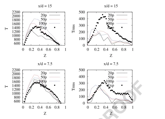
0 100 200 300 400 500
0 0.2 0.4 0.6 0.8 1
Trms
Z x/d = 7.5
20p 50p 100p Exp 0
100 200 300 400 500
0 0.2 0.4 0.6 0.8 1
Trms
Z x/d = 15
20p 50p 100p Exp
600 800 1000 1200 1400 1600 1800 2000 2200
0 0.2 0.4 0.6 0.8 1
T
Z x/d = 7.5
20p 50p 100p Exp 600
800 1000 1200 1400 1600 1800 2000 2200
0 0.2 0.4 0.6 0.8 1
T
Z x/d = 15
20p 50p 100p Exp
Fig. 9 Radial profiles of conditional temperature and rms at different axial locations with IEM
slightly more sensitive to the particle number density than MMC-Curl’s. The better agree- 333
ment with experimental data can be attributed to the fact that pair-wise models are known to 334
model mixing more realistically than mean based models. It is emphasized again, that for all 335
test cases the same mixing constant has been used, and no efforts have been made to control 336
mixing through the mixing time scale as is a common practice. This does not necessarily 337
imply that all the models have the best performance with the same constant. Adjustments 338
of the mixing constant Cφ could have led to more realistic degrees of extinction and can 339
have effects on the stability of the numerical solution but may deteriorate the mixing field 340
predictions [4] and would not aid the analysis of the differences between MMC-enhanced 341
mixing models and the particle number dependence. 342
The predictions of the radial profiles of temperature (not shown here) are generally less 343
sensitive to the number of particles for all models and the same holds for species such as 344
CH4. It can be noticed that for all the test cases the temperature predictions are satisfying 345
and a small improvement is noticed with the addition of MMC for radial positions r/d> 346
1.5 (towards the lean side of the flame). On the other hand the prediction of species such 347
as CO or H2O that are more sensitive to small changes of temperature is more challenging 348
and more dependent on the quality of the mixing model. Figures10and 11show the radial 349
profiles of CO at different axial locations. MMC shows less sensitivity to the particle num- 350
ber when compared to IEM and less noise than Curl’s, which indicates increased numerical 351
stability that was reported to be an issue in earlier PDF calculations when using IEM and 352
Curl’s mixing models [4,36]. MMC-Curl’s with 100 particles/cell gives the overall best 353
agreement. 354
IEM and MMC-IEM have opposite tendency when the particle number is increased at 355
x/d=15; the more particles are used in IEM, the higher the temperature, re-igniting the flame. 356
This is consistent with the scatter plot in Fig.4where the lower branch disappears as the 357
number of particles increases. MMC-IEM have a much more uniform behaviour, with min- 358
imum difference in temperature predictions with particle refinement. Doubling the number 359
[image:14.440.100.389.53.261.2]UNCORRECTED
PR
OOF
0 0.01 0.02 0.03 0.04 0.050 1 2 3 4 5 6
CO r/D x/D=7.5 20p 50p 100p Exp 0 0.01 0.02 0.03 0.04 0.05
0 1 2 3 4 5 6
CO r/D x/D=15 20p 50p 100p Exp 0 0.01 0.02 0.03 0.04 0.05
0 1 2 3 4 5 6
CO r/D x/D=30 20p 50p 100p Exp 0 0.01 0.02 0.03 0.04 0.05
0 1 2 3 4 5 6
CO r/D x/D=7.5 20p 50p 100p Exp 0 0.01 0.02 0.03 0.04 0.05
0 1 2 3 4 5 6
CO r/D x/D=15 20p 50p 100p Exp 0 0.01 0.02 0.03 0.04 0.05
0 1 2 3 4 5 6
CO r/D x/D=30 20p 50p 100p Exp
Fig. 10 Radial profiles of CO at different axial locations with MMC-IEM (left) IEM(right)
is amplified, when we look at CO predictions (see Fig.10) at x/d=15. At the same position
361
the MMC-IEM shows no particle number dependency, although it under-predicts extinction
362
as observed in Fig.8.
363
When the Curl’s mixing sub-model is used, both MMC-Curl’s and Curl’s exhibit large
364
particle dependency in and around the zone with significant extinction (see Fig.11). This
365
suggests that when extinction occurs, large numbers of particles per cell are indeed needed.
366
However, away from it, fewer particles per cell are needed in the MMC context as the
367
extra dependence on the reference space improves the mixing description. Probably more
368
than one reference space is needed when severe extinction occurs, a modification suggested
369
in previous studies as well [7,22]. In the case of Curl’s, large fluctuations are observed
370
even with 100 particles per cell, while MMC produces smoother statistics. This can be
371
easily understood by the nature of the corresponding SDE’s of the MMC and PDF methods,
372
Eqs.13and2, respectively. The diffusion coefficient of MMC equations can be zero locally,
373
unlike the PDF equations, and therefore statistical noise can be globally reduced.
374
An additional observation is that MMC shows better behaviour along the centreline and
375
this is probably due to a better numerical treatment of the conditional velocity close to the
376
centreline. It is not in the scope of this paper to explore the modelling of the conditional
[image:15.440.73.366.55.385.2]UNCORRECTED
PR
OOF
0 0.01 0.02 0.03 0.04 0.05
0 1 2 3 4 5 6
CO
r/D x/D=7.5
20p 50p 100p Exp 0
0.01 0.02 0.03 0.04 0.05
0 1 2 3 4 5 6
CO
r/D x/D=15
20p 50p 100p Exp 0
0.01 0.02 0.03 0.04 0.05
0 1 2 3 4 5 6
CO
r/D x/D=30
20p 50p 100p Exp
0 0.01 0.02 0.03 0.04 0.05
0 1 2 3 4 5 6
CO
r/D x/D=7.5
20p 50p 100p Exp 0
0.01 0.02 0.03 0.04 0.05
0 1 2 3 4 5 6
CO
r/D x/D=15
20p 50p 100p Exp 0
0.01 0.02 0.03 0.04 0.05
0 1 2 3 4 5 6
CO
r/D x/D=30
20p 50p 100p Exp
Fig. 11 Radial profiles of CO at different axial locations with MMC-Curl’s (left) Curl’s (right)
velocity, however, it can be briefly noticed from Eq.15and18that the fluctuating part of 378
the velocity becomes zero when the gradients of mixture fraction are zero allowing particles 379
to follow the mean flow field trajectories. 380
5 Conclusion
381In this paper we suggest a numerical framework for modelling the mixing term of the joint- 382
scalar PDF. Two models are tested for the prediction of the degree of extinction of a piloted 383
non-premixed turbulent methane flame close to blow off. The behaviour of two new mixing 384
models has been assessed in the MMC context and compared to common mixing models 385
in the literature. The models suggested in this work are extensions of two classic mixing 386
models (Curl’s and IEM) and aspire to overcome the deficiencies of the classical models 387
modelling of flames close to extinction. The results indicate that by introducing to the Curl’s 388
and IEM model indirect localness in the mixture fraction space through the use of the ref- 389
erence space, the predictions’ sensitivity to the number of particles is reduced. This trend 390
is more pronounced for the MMC-IEM variation of the model. For all test cases no efforts 391
[image:16.440.72.370.54.386.2]UNCORRECTED
PR
OOF
and the same constant was used. Although it is well known that adjustments of the mixing
393
constantCφ could have led to more realistic degrees of extinction this would diminish the
394
assessment of the predictive capabilities of the MMC-enhanced mixing models in terms of
395
particle number dependence.
396
Acknowledgments Support is acknowledged from Deutsche Forschungsgemeinschaft (DFG) under grant
397
number KR3684/7-1. Dr Vogiatzaki would like to acknowledge the contribution of The Lloyds Register 398
Foundation. Lloyds Register Foundation helps to protect life and property by supporting engineering-related 399
education, public engagement and the application of research. 400
References
401
1. Barlow, R., Frank, J.: Effects of turbulence on species mass fractions in methane/air jet flames. Proc. 402
Combust Inst 27, 1087–1095 (1998) 403
2. Barlow, R., Frank, J., Karpetis, A., Chen, J.Y.: Piloted methane/air jet flames: Transport effects and 404
aspects of scalar structure. Combust. Flame 143, 433–449 (2005) 405
3. Cao, R., Pope, S.: The influence of chemical mechanisms on pdf calculations of nonpremixed piloted jet 406
flames. Combust. Flame 143, 450–470 (2005) 407
4. Cao, R., Wang, H., Pope, S.: The effect of mixing models in pdf calculations of piloted jet flames. Proc. 408
Combust Inst 31, 15431550 (2007) 409
5. Chen, H., Chen, S., Kraichnan, R.: Probability distribution of a stochastically advected scalar field. Phys. 410
Rev. Lett. 63(24), 2657–60 (1989) 411
6. Sung, C.J., Law, C., Chen, J.: Augmented reduced mechanisms for no emission in methane oxidation. 412
Combust. Flame 125(1–2), 906–919 (2001) 413
7. Cleary, M., Kronenburg, A.: Hybrid multiple mapping conditioning on passive and reactive scalars. 414
Combust. Flame 151(4), 623–638 (2007) 415
8. Corrsin, S.: J. Aeronaut. Sci. 18, 417 (1951) 416
9. Curl, R., Miller, R., Ralph, J., Towell, G.: Dispersed phase mixing: Ii. measurements in organic dispersed 417
systems. AIChE J. 9, 175–181 (1963) 418
10. Dopazo, C.: Probability density function approach for a turbulent heated jet. centerline evolution. Phys. 419
Fluids 18, 397–404 (1975) 420
11. Gardiner, C.: Handbook of stochastic methods. Springer, New York (1984) 421
12. Ge, Y., Cleary, M., Klimenko, A.: Sparse-lagrangian{FDF}simulations of sandia flame e with density 422
coupling. Proc. Combust. Inst. 33(1), 1401–1409 (2011) 423
13. Ge, Y., Cleary, M., Klimenko, A.: A comparative study of sandia flame series (df) using sparse-424
lagrangian{MMC}modelling. Proc. Combust. Inst. 34(1), 1325–1332 (2013) 425
14. Haworth, D.: Progress in probability density function methods for turbulent reacting flows. Prog. Energy 426
Combust. Sci. 36, 168259 (2010) 427
15. He, G.W., Zhang, Z.F.: Two-point closure strategy in the mapping closure approximation approach. Phys. 428
Rev. E 70(036), 309 (2004) 429
16. Janicka, J., Kolbe, W., Kollmann, W.: Closure of the transport equation for the probability density 430
function of turbulent scalar fields. J. Nonequil. Thermodyn 4, 47–66 (1979) 431
17. Klimenko, A.: Modern modelling of turbulent non-premixed combustion and reaction of pollution 432
emission. Proceedings of Clean Air VII, Lisbon, Portugal (2003) 433
18. Klimenko, A.: Matching the conditional variance as a criterion for selecting parameters in the simplest 434
multiple mapping conditioning models. Phys. Fluids 16(12), 4754–4757 (2004) 435
19. Klimenko, A.: On simulating scalar transport by mixing between lagrangian particles. Phys. Fluids 19(3), 436
31,702 (2007) 437
20. Klimenko, A., Bilger, R.: Conditional moment closure for turbulent combustion. Prog. Energy Combust. 438
Sci 25(6), 595–687 (1999) 439
21. Klimenko, A., Pope, S.: The modeling of turbulent reactive flows based on multiple mapping condition-440
ing. Phys. Fluids 15(7), 1907–1925 (2003) 441
22. Kronenburg, A., Cleary, M.J.: Multiple mapping conditioning for flames with partial premixing. 442
Combust. Flame 155, 215–231 (2008) 443
23. Launder, B., Spalding, D.: The numerical computation of turbulent flows. Comput. Methods Appl. Mech. 444
UNCORRECTED
PR
OOF
24. Lindstedt, R., Louloudi, S., Vaos, E.M.: Joint scalar probability density function modeling of pollutant 446 formation in piloted turbulent jet diffusion flames with comprehensive chemistry. Proc. Combust Inst 447
28(1), 149156 (2000) 448
25. Muradoglu, M., Jenny, P., Pope, S.B., Caughey, D.A.: A consistent hybrid finite-volume/particle method 449 for the pdf equations of turbulent reactive flows. J. Comp. Phys. 154, 342371 (1999) 450 26. Norris, A., Pope, S.: Turbulent mixing model based on ordering pairing. Combust. Flame 83(1–2), 27– 451
42 (1991) 452
27. Pope, S.: PDF methods for turbulent reactive flows. Prog. Energy Combust. Sci. 11(2), 119–192 (1985) 453 28. Pope, S.: Mapping closures for turbulent mixing and reaction. Theor. Comput. Fluid Dyn 2(5–6), 255– 454
70 (1991) 455
29. Pope, S.B.: A model for turbulent mixing based on shadow-position conditioning. Phys. Fluids 25(11) 456
(2013) 457
30. Raman, V., Pitsch, H.: A consistent les/filtered-density function formulation for the simulation of 458 turbulent flames with detailed chemistry. Proc Combust Inst 31, 1711–1719 (2007) 459 31. Subramaniam, S., Pope, S.: A mixing model for turbulent reactive flows based on euclidean minimum 460 spanning trees. Combust. Flame 115(4), 487–514 (1999) 461 32. Vogiatzaki, K., Cleary, M., Kronenburg, A., Kent, J.: Modeling of scalar mixing in turbulent jet flames 462 by multiple mapping conditioning. Phys. Fluids 21(2) (2009) 463 33. Vogiatzaki, K., Kronenburg, A., Navarro-Martinez, S., Jones, W.: Stochastic multiple mapping condi- 464 tioning for a piloted, turbulent jet diffusion flame. Proc. Combust Inst 33(1), 1523–1531 (2011) 465 34. Wandel, A., Klimenko, A.: Testing multiple mapping conditioning mixing for monte carlo probability 466 density function simulations. Phys. Fluids 17(12), 128,105 (2005) 467 35. Wandel, A.P., Lindstedt, R.P.: Hybrid multiple mapping conditioning modeling of local extinction. Proc. 468 Combust. Inst. 34(1), 1365–1372 (2013) 469 36. Xu, J., Pope, S.B.: Pdf calculations of turbulent nonpremixed flames with local extinction. Combust. 470