Optimal Trajectory Planning for Multiple Asteroid
Tour Mission by Means of an Incremental
Bio-Inspired Tree Search Algorithm
Aram Vroom
Faculty of Aerospace Engineering Delft University of Technology
Delft, The Netherlands Email: [email protected]
Marilena Di Carlo,
Juan Manuel Romero Martin
and Massimiliano Vasile
Department of Mechanical andAerospace Engineering University of Strathclyde Glasgow, United Kingdom Email: [email protected]
Abstract—In this paper, a combinatorial optimisation al-gorithm inspired by the Physarum Polycephalum mould is presented and applied to the optimal trajectory planning of a multiple asteroid tour mission. The Automatic Incremental Decision Making And Planning (AIDMAP) algorithm is capable of solving complex discrete decision making problems with the use of the growth and exploration of the decision network. The stochastic AIDMAP algorithm has been tested on two discrete astrodynamic decision making problems of increased complexity and compared in terms of accuracy and computational cost to its deterministic counterpart. The results obtained for a mission to the Atira asteroids and to the Main Asteroid Belt show that this non-deterministic algorithm is a good alternative to the use of traditional deterministic combinatorial solvers, as the computational cost scales better with the complexity of the problem.
I. INTRODUCTION
Discrete decision making problems are common problems within the field of engineering. For example, the design of a network, the scheduling of operations and the planning of a trajectory can be represented as combinatorial problems [1][2][3]. As the complexity of such problems increases with the growth of the set of decisions, it is favourable to develop efficient strategies to solve these problems. The algorithms that can solve these type of problems can be divided into two categories: deterministic and non-deterministic algorithms. Ex-amples of stochastic algorithms are ant colony optimisation, genetic algorithm and particle swarms [2], while deterministic algorithms are for example the branch-and-bound, tabu search and pattern search algorithms [4][5][6].
In this paper, a non-deterministic algorithm inspired by the Physarum Polycephalum mould is presented and applied to two problems in the field of astrodynamics. For a comparison between the Physarum algorithm, Branch and Cut and Genetic Algorithms, on the solution of Multi Gravity Assist trajectory problems, the interested reader can refer to [3][7].
Although various strategies based on this type of algorithm were previously developed to solve among others the shortest
path problem and to obtain the trajectory for a multi-gravity assist mission, these algorithms were either non-generic, or not made public [3][8][9]. As such, it was decided to develop a more general version of the algorithm that is capable of solv-ing various complex discrete decision maksolv-ing problems. The developed method has been named the Automatic Incremental Decision Making And Planning (AIDMAP) algorithm and has been integrated into the open-source SMART-O2C toolbox developed by the Advanced Space Concepts Laboratory of the University of Strathclyde. It is therefore freely available under the MPL2.0 license on https://github.com/strath-ace/ smart-o2c.
The AIDMAP algorithm and its operators are first described in Section II. In Section III, the developed algorithm is applied to two case studies. These case studies include a mission to the Atira asteroids and a mission to the Main Asteroid Belt. The goal of the former case study is to compare AIDMAP against a deterministic branch and prune strategy while the goal of the latter case study is to apply AIDMAP to a decision making problem with a large database of possible decisions. Section IV describes the benchmarking of the algorithm to measure the convergence speed versus the success rate. Finally, a number of conclusions are drawn in Section V.
II. AUTOMATICINCREMENTALDECISIONMAKINGAND PLANNINGALGORITHM
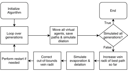
Fig. 1. The flowchart describing the AIDMAP algorithm
nodes connected by veins can resemble the set of consecu-tive decisions present in the aforementioned discrete decision making problems.
The pseudo-code of the algorithm is shown in Algorithm 1 and a flowchart of the algorithm can be seen in Figure 1. In the following sections, the various steps and operators of the algorithm are described in detail.
Algorithm 1 AIDMAP Algorithm
1: initialise algorithm variables 2: foreach generationdo
3: foreach virtual agentdo
4: whileend condition not reached do
5: create & evaluate decision paths (see Sec. II-B) 6: calculate probabilities (Eqs. 2, 3)
7: probabilistically choose next node 8: move agent to node
9: ifend condition reachedthen
10: save agent’s path as a solution
11: end if
12: end while
13: dilate vein radii (Eq. 4) 14: end for
15: increase vein radii in best path so far (Eq. 5) 16: simulate evaporation (Eq. 6)
17: ifvein radius outside of limitsthen
18: vein radius = limit 19: end if
20: ifrestart condition (see Sec. II-F) then
21: reset vein radii
22: update fluxes and probabilities 23: end if
24: end for
A. Virtual Agents
As can be seen on lines 1 to 3 in Algorithm 1, the algorithm starts with an initialisation, after which the nested loop over all generations and virtual agents is started. The amount of generations and virtual agents is specified by the user.
During each generation the predefined number of virtual agents are moved across nodes. As noted earlier, these virtual agents resemble nutrients as they move through the veins and encourage the growth and exploration of the decision network.
B. Decision Network Growth
When a virtual agent arrives at a node, it will first attempt to create a predefined number of decision paths to nodes that are not yet connected to the node the virtual agent is currently evaluating.
To do so, a loop is used that constructs new nodes, checks their validity and their potential to connect to the current node. This process continues until no more possible nodes are found, a maximum number of attemptsFf indmax have been made to
find new nodes or the specified number of ramification nodes kram have been generated.
During the generation of new nodes, each node is assigned a number of problem-specific attributes, a vein length, an initial radius defined by the user and a flux, and its validity is checked. The flux is calculated using a variation on the equation proposed in various previous papers on the Physarum Polycephalum and the classical Hagen-Poiseuille equation for the volumetric flow rate through a cylindrical duct with a certain length [10][11][12]. The equation used in the algorithm can be seen in Equation 1:
Qij =
πr4
ij
8µ 1 Lij
(1)
where rij is the radius of the vein from node i to node j,
µ is the fluid viscosity, Lij is the vein’s length and Qij is
the flux going through the vein. From this equation, one can see that as the length and radius increase, the amount of flux decreases and increases respectively. By defining a larger flux as being more favourable, one can set the length of the vein equal to the cost of the connection between the two nodes. As the fluid viscosity µ and the initial radius upon creation are defined by the user as well, and the vein length is found using a cost function provided by the user, the flux through a vein can now be found. The node’s problem-specific attributes are determined using a second file specified by the user. This generation of potential decision paths corresponds to line 5 in Algorithm 1. If the required number of valid ramification nodes has been generated, no more possible nodes are found or a maximum number of attempts to find a valid ramification nodeFf indmaxhave been made, the algorithm decides whether
to grow or further explore the decision network
C. Decision Network Exploration
In order to decide whether an agent moves to grow the decision network or to explore it, the flux calculated using Equation 1 is used.
First, as shown in line 6 of Algorithm 1, the probability of the agent moving from node i to nodej is calculated using Equation 2:
Pij =
Qλijcj ∑
j∈NiQ
λcj ij
(2)
In this equation,Pij is the probability of moving from nodei
to nodej,Qij is the flux flowing through the vein from node
i to node j, Ni is the total number of potential nodes that
andcj is a constant that is1for nodes that are not yet linked
to the current node, and 0 otherwise.
Once the probability has been found, it is weighted using Equation 3 to find the actual probability for an agent to move to node j [13]:
pij =
{
Pij(1−pram) if node is linked
Pijpram if node is not linked
(3)
where pram is the probability of ramification as defined by
the user. Using this probability, a non-deterministic choice is made by the agent when moving to the next node.
D. Vein Dilation
Once a virtual agent is no longer able to move or an end condition has been reached, the radius of the veins it has passed through is increased as shown in line 13 of Algorithm 1. This simulates dilation caused by the nutrients flowing through a vein. The dilation caused by agent k is modelled using Equation 4 [13]:
∆r(ijk)
dilation
=mr (k)
ij
L(totk)
(4)
wheremis the linear dilation coefficient andL(totk) is the total length of the veins traversed by agentk. It can be noted from Equation 2 that as this radius increases, the chance of another agent to move to the same vein increases. Once this dilation has been processed, the algorithm continues iterating over the agents that have not yet been moved.
E. cAMP Process & Vein Contraction
Once all the agents of a generation have moved, two additional processes are taken into account, being an additional vein dilation and contraction process. These correspond to lines 15 and 16 in Algorithm 1 respectively.
Firstly, it should be noted that the original Physarum algo-rithm was adapted to include another term in the dilation pro-cess that is based on the Dictyostelium Discoideum amoeba. When this amoeba starves, it starts to emit cyclic Adsenosine Monophosphate (cAMP) waves. As the other amoeba are sensitive to this chemical in their aggregative and slug stages, the result is that the amoeba start aggregating, thus showing collective behaviour [14]. In the AIDMAP algorithm, this starving amoeba is resembled by the agent with the best objective function, and the call for aggregation is simulated by a linear dilation of the vein radii of the best path. This can be seen in Equation 5 [13]:
∆rijbest
elasticity
=GF rijbest (5)
whereGF is the growth factor that is defined by the user and the subscript ijbest denotes all the veins of the best path.
Secondly, the evaporation is taken into account using Equa-tion 6 [13]:
∆rij
evaporation
=−ρrij (6)
One can see in this equation that once a generation has been completed, all radii over the entire graph are reduced by a factorρ, being the evaporation coefficient. In combination with Equation 5 and 4, the result of this is that veins that have not been traversed by any agents have their radius, and thus their probability, reduced.
As the vein dilation and contraction may lead to the radius of certain veins to be reduced to zero or to become too large, a check is performed to confirm whether the radius is outside of the bounds defined by a minimum and maximum radius set by the user. When this is the case, the radius is set to the minimum or maximum radius respectively. If one were to not perform this check, certain solutions could potentially be excluded or one solution could overpower the decision network [13].
F. Restart Procedure
Before the next generation is evaluated, a last check is performed. The reason for this is that, as every agent that moves through a certain vein increases the probability of that vein, there exists the risk of premature stagnation [13]. In order to prevent this premature stagnation, a restart procedure was implemented. This process works as follows: by comparing the path that each agent has travelled in a generation, it is checked whether two agents have at least ncom
min nodes in common.
If this is the case, the radii throughout the entire vein are reset to their initial values and the corresponding fluxes and probabilities are recalculated [13]:
rij=rini (7)
As shown in line 24 of Algorithm 1, the algorithm continues to the next generation once this conditions has been checked, thus closing the loop.
G. Algorithmic Complexity Considerations
Algorithm 1 shows that AIDMAP’s algorithmic complexity is equivalent to a standard ACO. This is clear also from the key mechanisms defined in Eqs. (1) to (6). Since AIDMAP simultaneously grows and explores the tree of decisions, the time complexity is not dependent on the number of nodes and branches. On the other hand, all parts of the tree are preserved in memory. Therefore, the memory allocation grows with the number of function evaluations.
III. CASESTUDIES
In order to test the algorithm described in Section II, two case studies have been evaluated. Both of the two case studies are related to the field of astrodynamics and mission analysis, and can be described as complex discrete decision making problems.
A. Low-Thrust Constrained Mission to the Atira Asteroids
As a first case study, a mission to the Atira asteroids is evaluated. This problem is based on the paper published by Di Carlo et al. in 2015 [15].
TABLE I
OVERVIEW OF THEAIDMAPPARAMETERS AND THEIR VALUES
Linear Dilation Coefficient m 1e-3 Evaporation Coefficient ρ 1e-4
Growth Factor GF 5e-3
Number of Agents Nagents 20
Number of Generations Ngenerations 200
Ramification Probability pram 0.7
Ramification Weight λ 1
Initial Radius rini 2
Minimum Radius rmin 1e-3
Maximum Radius rmax 5
Fluid Viscosity µ 1
Ramification Nodes kram 5
Max. Child Finding Attempts Ff indmax 1e4
Restart Threshold ncom
min 4
Earth orbit. However, these asteroids are difficult to study due to the limitations of the ground-based telescopes, as these can only detect the asteroids when the Sun is not in the field of view of the telescope. As these asteroids may form a significant threat to our planet, a mission was proposed to improve the knowledge of the Atira asteroids using a spacecraft [15]. Therefore, the objective in this case study is to visit as many Atira asteroids as possible, with the least amount of required change in velocity∆V. In order to prevent the need to use costly manoeuvres to change the spacecraft’s inclination, the nodal points of the considered asteroids are targeted [16]. The result of this, is that the spacecraft should arrive at the nodal point at the exact time that the asteroid is at this point in its orbit as well.
In the aforementioned paper, the final solution is obtained by first determining the optimal sequence of asteroids, departure times and arrival times using a branch-and-prune deterministic algorithm developed for discrete problems, called LambTAN (Lambert to Target Asteroids at Nodal points). The solution is found by using the patched conic approximation and modelling the transfer orbits as Lambert arcs [16]. Once the optimal sequence has been found, it is passed into a second algorithm that optimises the trajectory for the low-thrust spacecraft. In this case study, only sequence-finding will be considered.
To do so, each vein will represent the transfer from one celestial body to the next, while the nodes between two veins will contain the information on these transfers and the respective celestial bodies. Using this definition, the length shown in Equation 1 represents the∆V needed for the transfer. As such, when the required ∆V is lower, the amount of flux increases, thus in turn increasing the probability of the nutrient moving along the vein with a lower∆V.
1) Algorithm and Problem Settings: As can be noted from Section II, the algorithm requires the user to define a number of parameters. An overview of these parameters and the values used to solve this case study can be seen in Table I. The values shown in this table were obtained through the use of literature, testing and tuning [3][7].
As mentioned in Section II-B, the algorithm checks the validity of potential child nodes during the decision network growth process. To perform this check, a number of
problem-specific boundaries are tested. If either of these boundaries is not upheld, the potential child node is considered invalid and the algorithm will perform another attempt at finding a potential child node.
Firstly, it is tested whether the departure date required to arrive at the asteroid at the specified epoch with the chosen time of flight does not lie in the past. This check is equivalent to confirming that the required departure date does not lie before the arrival date of the previous arc:
Tdeparck ≥Tarrarck−1 (8)
Secondly, the feasibility of translating the impulsive Lambert transfer to a low-thrust trajectory is tested. This is done using the following two constraints [15]:
T oFarckϵ≥C∆Varck (9)
T oFarckϵ≥
√ V2
0 −2VfV0cos
(π 2∆i
) +V2
f (10)
whereT oFarck is the time of flight of the Lambert arc, ϵ is
the acceleration of the spacecraft’s low-thrust engine,C is an empirical coefficient,∆Varckis the required∆V found for the
Lambert trajectory, ∆i is the change in inclination,V0 is the spacecraft’s velocity when it passes the previous asteroid and Vf is the velocity at the end of the Lambert arc. The latter of
these two equations is the so-called Edelbaum condition and it should be noted that in this equation,∆ican be set to zero due to the fact that only the nodal points of the asteroids are targeted [17].
As a fourth constraint, the minimum perihelion distance of 0.31 Astronomical Units (AU) discussed in the aforementioned paper is considered. Using Equation 11, this condition is checked [15]:
a(1−e)≥rpmin (11)
in which a is the semi-major axis of the spacecraft’s orbit, e is its eccentricity and rpmin is the predefined minimum
perihelion distance [17].
In order to encourage the algorithm to find more solutions with a larger number of asteroids, a limit was set on the time between the spacecraft passing an asteroid and the starting time of the next Lambert arc. This time is defined as the
waiting time Twait and its boundaries are checked using
Equation 12:
Twait≤Twaitmax (12)
Furthermore, for the algorithm to find manoeuvres that can be done using the spacecraft, a limit was also set on the departure ∆V:
∆Vdep≤Vmaxarck (13)
Lastly, as the spacecraft will only have a limited amount of fuel, an upper limit for the total ∆V required for the full trajectory was set:
∆Vtot≤∆Vmax (14)
TABLE II
PROBLEM PARAMETERS FOR THE MISSION TO THEATIRA ASTEROIDS
T0 01/01/2020
Tend 01/01/2030 T oFmin 35 days T oFstep 10 days T oFmax 365 days
Twaitmax 730 days
∆Vmaxarck 3 km/s from Earth
1.5 km/s from transfer orbits
∆Vmax 4 km/s rpmin 0.31 AU
ϵ 10−4 m/s2
C 2
TABLE III
THE OPTIMAL SOLUTION FOUND USING THEAIDMAPALGORITHM
Asteroid Tdeparc ToFarc[d] Tarrarc ∆V [km/s]
2013JX28 2020/09/29 205 2021/04/22 0.87 2006WE4 2022/05/14 215 2022/12/15 0.86 2004JG6 2023/06/04 245 2024/02/04 0.65 2012VE46 2024/09/21 255 2025/06/03 0.39 2004XZ130 2026/09/15 205 2027/04/08 0.74 2008UL90 2028/07/31 195 2029/02/11 0.30
Total: 3.81
is the mission starting time, Tend is the mission end time
andT oFmin,T oFstepandT oFmax denote the minimum and
maximum time of flight for the Lambert arc as well as the time step at which the time of flight is evaluated. While these values were obtained from the paper by Di Carlo et al., it should be noted that the minimum time of flight is different. The reason for this, is that the algorithm used in the paper by Di Carlo et al. to find the optimum time of flight, evaluates the time-frame in a backward motion from 365 days to 30 days, while using a time step of 10 days. Because of this, the minimum time of flight evaluated by this algorithm was 35 days [15]. As the program written for this case study evaluates the possible time of flights in an increasing fashion, the minimum time of flight has to be set to 35 days to be able to obtain the solution presented in the paper when the time step of 10 days is used.
2) Results: Using the settings shown in Tables I and II, the solution shown in Table III is obtained. In this table, Tdeparc and Tarrarc denote the departure and arrival times of
the Lambert arc, and ToFarc is the time of flight for this arc.
For ease of reference, the results obtained by Di Carlo et al. are shown in Table IV. Interesting to note from this table, is that the trajectory uses the same sequence of asteroids and dates for
TABLE IV
THE OPTIMAL SOLUTION FOUND BYDICARLO ET AL. [15]
Asteroid Tdeparc ToFarc[d] Tarrarc ∆V [km/s]
2013JX28 2020/09/29 205 2021/04/22 0.87 2006WE4 2022/05/14 215 2022/12/15 0.86 2004JG6 2023/06/14 235 2024/02/04 0.61 2012VE46 2024/09/11 265 2025/06/03 0.36 2004XZ130 2026/09/15 205 2027/04/08 0.73 2008UL90 2028/07/31 195 2029/02/11 0.34
Total: 3.77
TABLE V
THE ORBITAL ELEMENTS OF THE FOUR ADDITIONALATIRA ASTEROID
Asteroid: 2013TQ5 2014FO47 2015DR215 2015ME131
a [AU] 0.7737 0.7522 0.6664 0.8049
e [-] 0.1556 0.2711 0.4716 0.1989
i [deg] 16.3986 19.1980 4.0903 28.8765
Ω[deg] 286.7789 358.6600 314.9819 314.3638
ω[deg] 247.3049 347.4558 42.2604 164.0285 M0[deg] 232.5338 52.1090 50.8887 189.7431 t0 [MJD2000] 6055.5 6055.5 6055.5 5652.5
TABLE VI
THE OPTIMAL SOLUTION FOUND BY THEAIDMAPALGORITHM WHEN THE NEWLY DISCOVEREDATIRA ASTEROIDS ARE ADDED TO THE
DATABASE
Asteroid Tdeparc ToFarc[d] Tarrarc ∆V [km/s]
2015ME131 2020/01/10 195 2020/07/23 0.61 2014FO47 2021/04/15 285 2022/01/25 0.54 2008UL90 2022/03/19 195 2022/09/30 0.27 2004JG6 2023/03/16 325 2024/02/04 0.65 2013JX28 2024/04/12 275 2025/01/12 0.62 2012VE46 2025/01/19 135 2025/06/03 0.35 2010XB11 2026/11/24 195 2027/06/07 0.77 2006WE4 2028/07/16 245 2029/03/18 0.18
Total: 3.99
the arrival times as found by Di Carlo et al., and that the time of flight of the Lambert arcs is similar to those presented in the paper for all but the 3rdand4tharc, causing the required
∆V to be 0.04 km/s higher. However, as the 3rdarc is 10 days
more than the one presented in the paper and the 4th arc is
10 days less, this difference cancels itself out with respect to the departure times, thus resulting in the departure times also being similar for all but these arcs. It should be mentioned that for the 5th and 6th arcs, while the departure dates, time
of flights and arrival dates are equal to those presented in the paper, the∆V needed for these manoeuvres was found to be 0.01 km/s larger and 0.04 km/s smaller than the ones shown in the paper by Di Carlo et al. The cause of this, is a minor difference in the initial starting position. This small difference propagates through the solution, slightly changing the required orbit, in turn causing the Lambert arcs to change as well.
In an attempt to further evaluate the mission’s potential, four additional Atira asteroids that have been discovered since the paper was published were added to the database as well. The osculating orbital elements of these four Atira asteroids can be seen in Table V [18]. The optimal solution found when these four additional Atira asteroids have been added to the database can be seen in Table VI. As expected, the adding of additional target asteroids for the spacecraft to move to increases the total number of asteroids that can be visited within the mission time. However, while this solution is capable of visiting 2 additional asteroids, the required ∆V is also 0.18 km/s higher.
B. Low-Thrust Constrained Mission to the Main Asteroid Belt
TABLE VII
OVERVIEW OF THEAIDMAPPARAMETERS AND THEIR VALUES USED FOR THE MISSION TO THEMAINASTEROIDBELT
Linear Dilation Coefficient m 5e-3 Evaporation Coefficient ρ 1e-3
Growth Factor GF 5e-3
Number of Agents Nagents 10
Number of Generations Ngenerations 40
Ramification Probability pram 0.7
Ramification Weight λ 1
Initial Radius rini 2
Minimum Radius rmin 1e-3
Maximum Radius rmax 5
Fluid Viscosity µ 1
Ramification Nodes kram 5
Max. Child Finding Attempts Ff indmax 2e4
Restart Threshold ncom
min 5
TABLE VIII
RANGE OF ORBITAL ELEMENTS FOR THE SPACECRAFT’S INITIAL ORBIT USED FOR THE COMPUTATION OF THEMOIDWITH THE ASTEROIDS
rp[AU] ra[AU] i[deg] Ω[deg] ω[deg]
1 [2.36, 3.20] [0, 35] 0 [0, 360]
case, the objective is also to visit as many asteroids as possible within the time frame, with the least amount of ∆V. The problem assumes the same acceleration as used in the mission to the Atira asteroids, being 10−4 m/s2. The time-frame for the mission starts at 02/01/2029 and ends on 02/01/2049.
1) Algorithm and Problem Settings: The settings shown in Table I were adapted through testing, in order to cope with the increased complexity of the problem while having access to the same computational resources. The values used instead for this case study are shown in Table VII. Moreover, other mission related parameters need to be defined before AIDMAP can be applied to the problem. In particular, the initial orbit and the various boundaries on time and ∆V need to be set. The definition of the initial orbit for the mission to the Main Asteroid Belt is based on the concept of the Minimum Orbital Intersection Distance (MOID) between the spacecraft’s orbit and the asteroids’ orbits [19]. The MOID is computed for a time period of 20 years. The database of asteroids in the Main Belt with diameter greater than 10 km and different possible initial orbits is considered. The possible orbital elements considered for the initial spacecraft orbit are given in Table VIII.
For each possible initial orbit of the spacecraft, the aster-oids with MOID < 0.01 AU with respect to this orbit are sought. For the combinations of initial orbits and asteroids that satisfy this condition, the relative phasing is also considered, propagating the orbits of both spacecraft and asteroids. This process allows one to identify an initial orbit with close encounters (MOID<0.01) to many asteroids in the database. In particular the orbit characterised by orbital elements rp =
1 AU, ra = 3.1066AU,i=0 deg,Ω= 0 deg,ω = 150and
M0= 101deg on 01/01/2030 has both MOID<0.01 and the condition on orbital phasing satisfied for the encounter with 37 asteroids in the database. This orbit is therefore the chosen
initial orbit for use in the AIDMAP algorithm.
As for the problem boundaries, the same boundary parame-ters need to be defined as done for the first case study. In this case, the maximum∆V for an individual transfer arc was set to be 0.75 km/s, the maximum total∆V was set to 5 km/s and the empirical coefficientCwas assumed to be 2. For the minimum and maximum time of flight, the boundaries were set to be 4 days and 730 days, using a time step of 10 days. These limits were found from the results obtained by the computation of the closest encounters between the spacecraft and asteroids. In particular the minimum and maximum total time between two encounters was found to be 4 days and 1064 days respectively. By setting the maximum time of flight and waiting time to both be equal to 730 days, one allows for the total time between encounters to be 1064 days plus an additional margin for the transfer orbit. The latter is needed due to the fact that the initial orbit defined above does not necessarily get sufficiently close to the asteroid, since it only guarantees that the MOID is lower than 0.01 AU. The AIDMAP algorithm on the on the other hand will attempt to intersect the orbit with the asteroid’s centre, hence requiring a margin for the total transfer time.
It should be noted that for this case study, Equation 9 was slightly altered. Namely, Equation 15 is used instead:
(T oFarck+Twaitk−Tmeas)ϵ≥C∆Varck (15)
In this equation, it may be noticed that two additional terms have been added. Firstly, the waiting time was included due to the fact that low-thrust engine could also provide thrust during the waiting time, thus slightly relaxing the constraint. However, another term Tmeas was introduced to ensure that
the low-thrust engine does not need to be turned on during the time that measurements are performed near the asteroid. In this problem,Tmeas was set to be 20 days.
Aside from that, the boundary shown in Equation 10 is ignored in this case study, as the Edelbaum shown here is only valid for near-circular orbits [17]. As the initial orbit used in this case study is significantly eccentric, as opposed to the orbit used in the first case study, this boundary is not taken into account.
2) Results: The solution obtained using the parameters stated in Tables I and II can be found in Table IX. In this table, Tdeparc, Tarrarc and ToFarcdenote the departure time, arrival
time and time of flight of the Lambert arc respectively. It can be seen in this table that the resulting trajectory is capable of visiting 11 out of the 37 considered asteroids, and that the total∆V is 2.94 km/s.
TABLE IX
THE TRAJECTORY FOUND FOR THE MISSION TO THEMAINASTEROID
BELT
Asteroid Tdeparc ToFarc[d] Tarrarc ∆V [km/s]
1906VP 2029/02/20 724 2031/02/14 0.20 Klytia 2032/07/03 634 2034/03/29 0.10 1939TA 2034/04/25 644 2036/01/29 0.23 1935OB 2036/05/20 404 2037/06/28 0.70 1905PS 2037/11/09 364 2038/11/08 0.08 1925TD 2038/11/15 334 2039/10/15 0.47 1902LK 2040/04/25 484 2041/08/22 0.38 Kassandra 2041/09/28 384 2042/10/17 0.15 1978QP1 2043/10/20 364 2044/10/18 0.25 1935MG 2046/04/19 374 2047/04/28 0.14 1973FF1 2047/06/04 364 2048/06/02 0.23
Total: 2.94
TABLE X
THE TRAJECTORY FOUND WHEN THE FULL ASTEROID DATABASE IS USED AS INPUT
Asteroid Tdeparc ToFarc[d] Tarrarc ∆V [km/s]
1992UU 2029/09/28 684 2031/08/13 0.17 1908DH 2032/07/18 574 2034/02/12 0.38 1905QD 2035/02/21 274 2035/11/22 0.20 1905PS 2037/01/03 674 2038/11/08 0.58 1902LK 2040/04/05 504 2041/08/22 0.24 Asia 2041/11/18 534 2043/05/06 0.40 1978QP1 2043/10/30 354 2044/10/18 0.24 1892N 2044/11/26 514 2046/04/24 0.04 1924QL 2046/08/02 384 2047/08/21 0.33 1906TP 2047/08/25 234 2048/04/15 0.75
Total: 3.33
From this table, it can be observed that the best solution is capable of visiting 10 asteroids using a∆V of 3.33 km/s. By comparing this solution with the one shown in Table IX, it can be concluded that using the database of the 37 asteroids as input for the algorithm, as opposed to the full database of 1977 asteroids, is indeed effective when the settings shown in Table VII are used. In order to be able to cope with the larger dataset, a larger number of agents and generations are needed to sufficiently explore the search space.
IV. BENCHMARKING
To evaluate the efficiency of the AIDMAP algorithm, the original algorithm used in the paper by Di Carlo et al. was compared to the algorithm discussed in this paper.
LambTAN is a deterministic algorithm that takes inspira-tion from a combinainspira-tion of the branch-and-prune algorithm and the incremental pruning discussed in [20] and [21]. In essence, LambTAN branches out through the search space and constructs and assesses transfers arcs one after another. If a solution is found to be non-feasible, the branch is pruned [15]. The comparison is done by evaluating the number of func-tion evaluafunc-tions and the success rate of AIDMAP assuming that the solution provided by LambTAN is the reference. This is reasonable as the solution generated by LambTAN was obtained with a nearly exhaustive deterministic search.
The use of AIDMAP is considered successful if the final solution has the same sequence as the one found by the Lamb-TAN algorithm and if the ∆V found is at most 5, 10 or 15
50 75 100 125 150 175 200
Generations 0
0.1 0.2 0.3 0.4 0.5 0.6 0.7 0.8
Success Rate
5 Percent 10 Percent
[image:7.612.329.541.262.434.2]15 Percent
Fig. 2. The success rate of the AIDMAP algorithm as a function of the number of generations when the settings shown in Tables I and II are used
50 75 100 125 150 175 200
Generations
0.9 1 1.1 1.2 1.3 1.4 1.5 1.6 1.7 1.8 1.9
Function Evaluations
×106
95% Confidence Int. Dataset Boundaries Mean
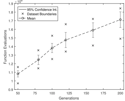
Fig. 3. The number of function evaluations performed by the AIDMAP algorithm when a set number of generations is evaluated and the settings shown in Tables I and II are used
percent larger than the one found by the LambTAN algorithm. The trends of success rate versus number of generations can be found in Figure 2. To obtain this graph, the values shown in Tables I and II were used as inputs, and a dataset of 40 runs was used for each data point.
From this graph, it can clearly be seen that the success rate increases as the number of generations increases. However, it can also be noted that with a boundary of 5 percent, the success rate at 100 and 160 generations is lower than one would expect from observing the trend. The cause of this is likely to be the limited size of the dataset. Nonetheless, the trend observed here is similar to the one of other Physarum-based algorithms [3]. As for how the amount of function evaluations changes with the amount of generations, this can be seen in Figure 3. In this figure, a function evaluation is defined as a call to the cost function.
performed when a lower or higher number of generations is used. The cause of this, is the non-deterministic nature of the algorithm; the number of function evaluations performed when a certain number of agents and generations is selected is not a set value.
To compare these statistics with LambTAN’s, it should be mentioned that LambTAN performs 6.9·107 function evalua-tions to obtain the solution. It can be noted that this is more than a factor 30 larger than the amount of function evaluations performed by the AIDMAP algorithm when 20 agents, 200 generations and the settings shown in Tables I and II are used. While LambTAN is guaranteed to succeed due to the fact that it is evaluating all available trajectories, it becomes highly inefficient to use LambTAN when the dataset of possible asteroids increases significantly. Due to this disadvantage of LambTAN and the increasing need for algorithms that can efficiently solve large and complex combinatorial problems, the AIDMAP algorithm can certainly be considered a valuable alternative.
V. CONCLUSION
In this paper, the bio-inspired Automatic Incremental De-cision Making And Planning (AIDMAP) algorithm has been presented and its operators have been described. The proposed algorithm has furthermore been applied to two discrete deci-sion making problems in the field of astrodynamics.
In the first case study, it has been shown that the AIDMAP algorithm is capable of accurately reproducing the optimal trajectory to six Atira asteroids found using an alternative deterministic algorithm, and that the AIDMAP algorithm is capable of finding a new optimal solution when the database is updated with a set of newly discovered Atira asteroids.
In the second case study, a mission to the Main Asteroid Belt, it has been demonstrated that, by first using the Minimum Orbital Intersection Distance to find the optimal starting orbit and potential set of visitable asteroids, the AIDMAP algorithm can effectively find an optimal solution for a discrete decision making problem with an increased level of complexity.
To benchmark the AIDMAP algorithm, the number of generations used by the AIDMAP algorithm in the first case study was varied and the number of function evaluations and success rate was compared to those of the deterministic LambTAN algorithm. It has been shown that, while LambTAN always succeeds in finding the optimal solution, the number of function evaluations it requires is more than a factor 30 larger than the amount of function evaluations performed by the AIDMAP algorithm in the test presented in this paper. Due to the increasing need for algorithms that can efficiently handle large scale combinatorial problems, it can be concluded that the AIDMAP algorithm provides, at comparable accuracy of the solutions found, a more efficient alternative to the currently existing deterministic algorithms.
REFERENCES
[1] A. Tero, et al., “Rules for biologically inspired adaptive network design.”
Science (New York, N.Y.), vol. 327, no. 5964, pp. 439–42, 1 2010. [2] S. S. Rao,Engineering optimization : theory and practice, 4th ed. John
Wiley & Sons, 2009.
[3] L. Masi and M. Vasile, “A multidirectional Physarum solver for the automated design of space trajectories,” in 2014 IEEE Congress on Evolutionary Computation (CEC). IEEE, 7 2014, pp. 2992–2999. [4] E. L. Lawler and D. E. Wood, “Branch-and-bound methods: A survey,”
Operations Research, vol. 14, no. 4, pp. 699–719, 1966.
[5] F. Glover and M. Laguna,Tabu Search. New York, NY: Springer New York, 2013, pp. 3261–3362.
[6] R. Hooke and T. A. Jeeves, ““ direct search” solution of numerical and statistical problems,”J. ACM, vol. 8, no. 2, pp. 212–229, Apr. 1961. [7] M. Vasile and V. M. Becerra,Computational intelligence in aerospace
sciences, ser. Progress in Astronautics and Aeronautics, 2014. [8] X. Zhang, Q. Wang, A. Adamatzky, F. T. S. Chan, S. Mahadevan,
Y. Deng, X. Zhang, Q. Wang, A. Adamatzky, F. T. S. Chan, S. Mahade-van, and Y. Deng, “An improved Physarum polycephalum algorithm for the shortest path problem,”The Scientific World Journal, vol. 2014, p. 487069, 2014.
[9] L. Liang Liu, Y. Yuning Song, H. Haiyang Zhang, H. Huadong Ma, and A. V. Vasilakos, “Physarum Optimization: A Biology-Inspired Al-gorithm for the Steiner Tree Problem in Networks,”IEEE Transactions on Computers, vol. 64, no. 3, pp. 818–831, 3 2015.
[10] D. S. Hickey and L. A. Noriega, “Insights into Information Processing by the Single Cell Slime Mold Physarum Polycephalum,” inUKACC Control Conference Proceedings, Manchester, UK, 2008.
[11] A. Tero, K. Yumiki, R. Kobayashi, T. Saigusa, and T. Nakagaki, “Flow-network adaptation in Physarum amoebae,”Theory in Biosciences, vol. 127, no. 2, pp. 89–94, 5 2008.
[12] A. Tero, R. Kobayashi, and T. Nakagaki, “Physarum solver: A biologi-cally inspired method of road-network navigation,”Physica A: Statistical Mechanics and its Applications, vol. 363, no. 1, pp. 115–119, 2006. [13] J. M. R. Martin, M. Vasile, L. Masi, E. Minisci, R. Epenoy, V. Martinot,
and J. F. Baig, “Incremental planning of multi-gravity assist trajectories,”
Acta Astronautica, vol. 115, pp. 407–421, 2015.
[14] R. L. Chisholm and R. A. Firtel, “Insights into morphogenesis from a simple developmental system,”Nature Reviews Molecular Cell Biology, vol. 5, no. 7, pp. 531–41, 07 2004.
[15] M. Di Carlo, N. Ortiz G´omez, J. M. Romero Martin, C. Tardioli, F. Gachet, K. Kumar, and M. Vasile, “Optimized low-thrust mission to the atira asteroids,”25th AAS/AIAA Space Flight Mechanics Meeting, pp. AAS15–299, 2015.
[16] R. R. Bate, D. D. Mueller, and J. E. White,Fundamentals of astrody-namics. Courier Corporation, 1971.
[17] V. A. Chobotov,Orbital mechanics. American Institute of Aeronautics and Astronautics, 2002.
[18] Jet Propulsion Laboratory. (2016) Small-Body Database Search Engine. [Online]. Available: http://ssd.jpl.nasa.gov/
[19] G. F. Gronchi, “An Algebraic Method to Compute the Critical Points of the Distance Function Between Two Keplerian Orbits,” Celestial Mechanics and Dynamical Astronomy, vol. 93, no. 1-4, pp. 295–329, 9 2005.
[20] V. M. Becerra, D. R. Myatt, S. J. Nasuto, J. M. Bishop, and D. Izzo, “An Efficient Pruning Technique for the Global Optimisation of Mul-tiple Gravity Assist Trajectories,” inProceedings of the International Workshop on Global optimization, San Jos, Almera, Spain, 2005. [21] D. Novac and M. Vasile, “Incremental solution of LTMGA transfers