Graph-based clustering for identifying region of interest in eye tracker data analysis

Graph-based clustering for identifying region of

interest in eye tracker data analysis

Kanghang He, Cheng Yang, Vladimir Stankovic, and Lina Stankovic

University of Strathclyde, Glasgow, G1 1XW, UK

Email:{kanghang.he, cheng.yang, vladimir.stankovic, lina.stankovic}@strath.ac.uk

Abstract—Localization of a viewer’s region of interest (ROI) on eye gaze signal trajectories acquired by eye trackers is a widely used approach in scene analysis, image compression, and quality of experience assessment. In this paper, we propose a novel clustering approach for ROI estimation from potentially noisy raw eye gaze data, based on signal processing on graphs. The clustering approach adapts graph signal processing (GSP)-based classification by first cleverly selecting a starting data sample, and then classifying the remaining samples. Furthermore, Graph Fourier Transform is used to adjust GSP parameters on-the-fly to maximise accuracy. Experimental results show competitive clustering accuracy of our proposed scheme compared to Density-based spatial clustering of applications with noise (DB-SCAN), Distance-Threshold Identification (I-DT), and Mean-Shift on publicly available Shape Dataset and the potential of estimating ROI accurately on true eye tracker data1_.

I. INTRODUCTION

When an image or scene is viewed, the eye gaze tends to pause on small regions within the image, called fixation areas. On average, fixations last for around 200 ms during the reading of linguistic text, and 350 ms during the viewing of a scene [1]. Existing approaches for detecting Region of Interest (ROI) in the viewed image first represent the centre of a fixation area as a fixation point [2], and then use clustering to group these fixation points from all fixation areas into spatial regions, identified as ROI. Various clustering approaches have been used to detect ROI, such as k-means and distance threshold [3], [4], Density-based spatial clustering of applications with noise (DB-SCAN) [5], Distance-Threshold Identification (I-DT) [6] and Mean-shift [7]. The gaze data, acquired by commercial eye trackers, is normally affected by high level of measurement noise and contains missing data due to eye blinks and occasional head movements. This motivates the use of Graph Signal Processing (GSP), an emerging field used to represent irregular data structures on graphs [8], [9], for robust gaze data clustering.

GSP is proposed for dataset classification in [10], where each dataset sample is associated with a graph vertex. The underlying graph is then designed to capture dependency between the data samples, by connecting samples/vertices that are highly correlated with high-weight edges. GSP-based classification is competitive to other machine learning based classification approaches, such as Support Vector Machines, when the data samples are noisy and/or training dataset is of

1_{978-1-5090-3649-3/17/$31.00 2017 IEEE}

poor quality or size, since GSP generates a graph based on intuition instead of relying on training (see [11]). GSP-based classification is used for image and text classification [10], energy disaggregation [12], motion classification [13], and many other signal/image processing tasks (see [9], [12], [14] and references therein). In [14] the GSP-based classification is extended to clustering for energy disaggregation by searching for vertices that have high similarities and grouping them into a cluster.

To identify ROI from noisy eye tracker data, in this paper, we first pre-process the eye tracker measurements, comprising the time-stamped eye gaze locations in the viewed image, by filtering the data to ensure convergence to locations of higher density, similarly to [7], and then cleverly choosing a data sample as a starting point for clustering. Then we propose a GSP-based iterative clustering method, for spatial clustering of pre-processed eye tracker data to detect ROI. Clustering is performed on the graph, where each graph vertex is associated to one spatial gaze measurement, that defines horizontal and vertical position of the gaze, and weights of the edges reflect spatial correlation between the measurements.

Note that, we focus on detection of ROI in still images, where an ROI is a group of gaze measurement spatially con-centrated regardless of the time information [7]. Having this in mind, and due to GSP’s resilience to noise, we bypass the traditional step of first finding time-dependent fixation points prior to ROI detection, making the proposed method robust to timing jitter and synchronization problems. Moreover, the method is inherently robust to measurement noise and eye blinks, and no denoising or data cleaning steps, common for eye tracker data processing, are needed.

II. PROPOSEDMETHOD

A. System Overview

Let N be the total number of samples from eye tracker gaze data, and(x,y) ={(x1, y1), ...,(xN, yN)}be the spatial

locations of the samples in the viewed image. The objective is to group samples into clusters m ∈ {1, . . . , M}, where M is the total number of clusters which is unknown. Let c = {c1, . . . , cN} where ci = m if sample (xi, yi) belongs

to clusterm.

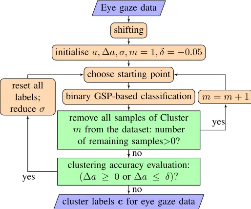
Fig. 1 shows the block diagram of the proposed GSP-based clustering method. First, similarly to [7], we perform preprocessing by shifting the input eye gaze data to make all samples move simultaneously towards locations of higher density (Section II-B). Then, one sample is cleverly chosen as the starting point to clustering (Section II-C). Next, a binary GSP-based classification is performed, similarly to [10] and [14], to classify all data samples into one of two classes: belonging to the same class as the starting point or not (Section II-C). All samples classified to the class of the starting point form Clusterm=1, and are removed from the dataset, a new starting point is chosen,m is incremented, and the process is repeated until no samples remain unclustered.

The cluster accuracy a (Section II-E), is then used to evaluate the quality of the formed clusters. If the accuracy improved compared to the previous iteration, then the under-lying graph used for GSP processing is adjusted, the clustering labels are reset and the process is repeated until accuracy cannot be further improved.

Eye gaze data

shifting

initialise a,∆a, σ, m= 1, δ=−0.05

choose starting point

binary GSP-based classification reset all

labels; reduceσ

m=m+ 1

remove all samples of Cluster m from the dataset: number

of remaining samples>0?

clustering accuracy evaluation:

(∆a ≥ 0 or∆a ≤ δ)?

cluster labels cfor eye gaze data yes

no

yes

no

Fig. 1. The proposed GSP-based clustering algorithm.

The pseudocode of the proposed method is shown in Algorithm 1.The following subsections provide a detailed description of each step.

B. Shifting Samples

Before clustering, a preprocessing operation, shif ting, is performed to make clustering robust to outliers, e.g.,

sac-cade points. This shifting step aims to move all samples to higher density locations, making samples in each cluster more compact. Let (x∗,y∗) = {(x∗₁, y∗₁), ...,(x∗_N, y∗_N)} denote the shifted data. For each sample (xi, yi), we define(x∗i, y∗i)as:

x∗_i =

Pb

n=1xn

b , (1)

y∗i =

Pb

n=1yn

b , (2)

where b is the number of most correlated neighbours to the vertex vi, i.e., we take the b highest-weight connections to

vertex vi. Fig. 2 shows an example of the raw data samples

and pre-processed, shifted samples. It is clear that the shifted points become more concentrated in each cluster.

Fig. 2. Comparison between shifted, preprocessed data and raw data.

C. Setting the Starting Point

Many ROI detection methods are based on randomly choos-ing the startchoos-ing point (see [7] and references therein); hence bad initial positions (e.g., saccade points) will rapidly reduce the clustering accuracy. We thus propose a method to refine the initial, random selection of the starting point. Let(xs, ys)

be a randomly chosen starting point. The shifted starting point x∗_sandy_s∗is calculated and updated using (1), (2) and until the difference between the points before and after shifting cannot be reduced anymore. The refined starting point(ˆxs,yˆs)is the

nearest sample to the final (x∗_s, y_s∗). Note that this way we ensure high point density around the selected starting point, hence the starting points is unlikely to be an outlier.

D. GSP-based Clustering

We use binary GSP-based classification to find samples that belong to the same class as (ˆxs,yˆs). We do this by first

constructing a graphG= (V,A), where for i= 2, . . . , N+ 1

each vertexvi∈ Vis associated with one data sample(x∗i, y∗i),

v1is associated with(ˆxs,yˆs), andAis the weighted adjacency

and vj, is defined using Euclidean distance with a Gaussian

kernel:

Ai,j= exp

(

−(x

∗

i −x∗j) 2_{+ (y}∗

i −yj∗) 2

σ2

)

, (3)

whereσis a scaling factor. Next, agraph Laplacianis defined as follows:

L=D−A, (4)

whereD is a degree matrix andDk,k=P N j=1Aj,k.

Starting from m = 1, we assume xˆs and yˆs belong to

Clustermand classify the remainingN samples as belonging to Cluster m or not. In particular, we initialize an (N+ 1) -length vector %as graph signal: %= [ς sm_]>_{,whereς = 1is}

associated with starting point( ˆxs,yˆs),smis anN-length row

vector initialised as all zeros.

Similar to [12], we adopt a Laplacian regularizer %>L% to measure the variation in signal sm _{with respect to the}

underlying graph, with the objective to find an sm∗ _that

minimizes the variation in the graph signal. The optimization problem

sm∗= arg min

sm ||% >_L%||2

2 (5)

has the following closed-form solution [15], [16], [17]:

sm∗=−L#_2:N+1,2:N+1ςL>_1,2:N+1, (6) where L#_2:N+1,2:N+1 is the pseudo-inverse of L2:N+1,2:N+1,

andsm∗_{∈[0,1]. Ifs}m i

∗_{is close to 1 (based on a heuristically}

set distance threshold), we designate that (x∗_i, y∗_i)belongs to the same cluster mas (ˆxs,yˆs), which we label asci=m.

Next, we remove all clustered points, increment m and repeat the procedure starting with selecting a new starting point (Sec. II-C) until all samples are labelled with a cluster number. Finally, the clusters that contain small fraction of samples, where the fraction parameter is denoted as α, are assumed to be outliers and all grouped to Cluster0. The cluster with coordinate(0,0)is also labelled as0since it contains all lost data caused by eye blinks and noise.

E. Self Parameter Tuning

Initial testing shows large dependency of the accuracy of the results on the scaling factor σdefined in (3) that weights the relationship between the data samples. Large σleads to large Ai,j indicating high correlation between the samples i and

j, which would result in many sample points being clustered together. Low σhas the opposite effect: small clusters would be formed comprising only highly correlated samples.

Since the bestσ, that is, the one that maximizes accuracy, is signal dependent, we propose a method for finding the optimal σbased on the signal samples. First,σis set to be a very high value, which leads to rough clustering (i.e., a small number of large clusters) for the giving dataset. After all samples are labelled following the procedure from the previous subsection, we define a graph signal for Cluster m,gm_as:

gm_i =1(ci==m). (7)

where1is an indicator function that returns1if the condition is true and0otherwise. We then calculate the graph Laplacian LG, which is symmetric, thus the signal value decomposition (SVD) ofLG is given by [18]:

LG=UΛU>, (8)

where Λ is a diagonal matrix with {λ0, λ1, . . . , λN−1} as

eigenvalues of LG on the diagonal, and U is a set of eigenvectors. The Graph Fourier Transform (GFT) of gm _is

then given by:

ˆ

gm_=U>_gm_{. (9)}

The eigenvalues of LG act as the graph frequencies and corresponding eigenvectors act as the graph harmonics [19], [20], [21]. Small λ’s carry information about low frequency components of the signal, while high frequencies (details) are carried by large λ’s. Motivated by the fact that high energy in the high frequencies indicate bad cluster quality, we estimate the frequency content of ˆgm

i as follows. Let

f = (λ0+λN−1)/2 and j∗ = arg minj|f−λj|, then λi

for i ≤j∗ would carry information about energy content in the lower half of the frequency spectrum.

Let rm be the ratio of the total number of low/high

fre-quency components ingˆm_{that are above/below a heuristically}

set threshold γai.e.,

rm=

PN

i=j∗₊₁ 1(|ˆgm_i |> γ)

Pj∗

i=1 1(|gˆim|> γ)

. (10)

rm > τ indicates a good cluster, where τ is a chosen

parameter. If not, all samples in this cluster are considered as incorrectly clustered. In addition, the samples with cluster label equal to 0 are also counted as incorrect samples. The estimated clustering accuracy is calculated as:

a= 1− κ

N, (11)

whereκ is the total number of incorrectly clustered samples that is given by:

κ=

N

X

i=1

1(x∗_i = 0 &y∗_i = 0)

+

N

X

i=1 M

X

m=1

1 (ci=m) & (

PN

i=1 1(ci=m)

N ≤α)

+

N

X

i=1 M

X

m=1

1 (ci=m) & (rm≤τ)

,

(12)

where the first line captures all samples in Cluster 0, the second line includes clusters that have very low number of samples (belowα), and the third line comes from all clusters that give rm < τ. The scaling factorσ is reduced by small

Algorithm 1: Proposed GSP-based spatial clustering. Input:(x,y);

Output:c;

1 set x∗_i via (1),y∗_i via (2),a= 0,∆a= 0,σ= 20, β = 0.99,τ= 5,b= 10,δ=−0.05,α= 0.03 ; 2 while ∆a≥0 or∆a≤δ do

3 set σ=σ−1,m= 1,c= 0;

4 while number of remaining samples>0do 5 randomly set (x_s, y_s);

6 compute(ˆxs,yˆs)as in Sec. II-C.;

7 computeA,L with(ˆxs,yˆs),(x∗,y∗), (3), (4);

8 computesm∗ via (6);

9 set c(findsm_i ∗> β) =m,m=m+ 1; 10 remove from the dataset samplesi with

sm_i ∗> β;

11 compute∆avia (10), (11), (12); 12 return c;

III. EXPERIMENTALRESULTS

In this section, we first validate the proposed spatial clus-tering algorithm on a public clusclus-tering dataset with known ground-truth labels, and show how the proposed clustering algorithm compares with DB-SCAN, I-DT and Mean-shift algorithms. Then we present the results with true eye tracker data to compare the accuracies of the four aforementioned methods in detecting ROI. Table I shows all parameters used for the proposed method in all experiments, which were heuristically obtained and are used for all datasets.

TABLE I

PARAMETER SETTINGS FOR THE PROPOSED METHOD USED IN ALL THE EXPERIMENTS.

symbol parameter setting

b neighbouring samples 10

τ cluster quality 5

σ scaling factor forA initially set 20

α sample fraction 0.03

β labelling threshold 0.99

δ accuracy difference threshold -0.05

γ frequency response 1₂max{|_gˆm i |}

A. Results with Shape Dataset

The four algorithms are first tested on the public Shape dataset [22], which is often used to assess accuracy of spatial clustering methods. The images in this dataset are scatter diagrams with labels, indicating the cluster index for each point, where the points close to each other are assigned to the same cluster.

Table II shows the clustering results of the four methods on the Shape dataset. The accuracy is measured as a ratio of the number of correctly clustered samples to the total number of samples. In DB-SCAN, the minimum number of points required to form a cluster and the number of neighbourhood samples of a point are denoted as andζ, respectively. The distance threshold in I-DT is denoted as η. The distance threshold and the number of neighbourhood samples of a point

TABLE II

CLUSTERING ACCURACY OF THE PROPOSED METHOD, DB-SCAN, I-DT ANDMEAN-SHIFT WITHOUT PREPROCESSING.

Proposed DB-SCAN I-DT Mean-shift

parameter Self-adaptable = 2 η= 5 σs= 7

σ ζ= 14 ρ= 10

R15 0.89 0.53 0.13 0.20

D31 0.76 0.06 0.30 0.35

Aggregation 0.79 0.88 0.87 0.89

Toy 0.30 0.91 0.46 0.48

Compound 0.84 0.90 0.69 0.78

Pathbased 0.80 0.85 0.67 0.66

Flame 0.95 0.35 0.95 0.91

Mean 0.76 0.64 0.58 0.61

in Mean-shift are denoted asσsandρ, respectively. Parameters

in DB-SCAN, I-DT and Mean-shift are tuned and fixed using a greedy search scheme to get best performance for the whole dataset. The proposed approach can self tune itself to find the best parameters for each image pattern.

The performance of DB-SCAN on some images, such as

Compound, is good. There are many individual points that are isolated in Compound dataset.They are all clustered as a single cluster in ground truth which DB-SCAN consider them as noise. However, since DB-SCAN is a density-based spatial clustering, it cannot adapt well to different point density characteristics of the images, leading to poor performance in some cases. I-DT is a distance-based method, where results are highly influenced by the size of clusters in the image. In Mean-shift all points are repetitively moved until converged to positions with high density [7]. Then, a distance threshold is applied to cluster the shifted points, while the size of the clusters is depended on σs. Thus, the overall performance is

poor due to variations in cluster sizes across the images. For some images, the ground-truth clusters are connected with consecutive points. In GSP-based clustering, these clus-ters will be treated as piecewise smooth signals since the weight is defined based on the distance between samples, and thus these clusters are incorrectly merged into the same cluster. Shift pre-processing can move these connecting points closer to their closest high density centres, disconnecting in this way the clusters, and leading to more effective clustering.

Table III shows the results of our proposed GSP-based clustering method compared with DB-SCAN, I-DT and Mean-Shift after shift preprocessing is applied on the images prior to running all 4 clustering algorithms. We again use a greedy search scheme to get the optimal parameters for all competing schemes. Overall performance for all methods except Mean-shift has improved compared to clustering the raw data without pre-processing. This proves that the shift preprocessing can significantly improve the clustering accuracy. For Mean-shift, the preprocessing does not improve the performance, since the effect of the proposed shift preprocessing is similar to the operation that is already done in the Mean-shift. Indeed, Mean-shift uses the weighted mean of nearby points based on the kernel function to make the samples compact.

B. Results on the Eye Tracker Dataset

TABLE III

CLUSTERING ACCURACY OF THE PROPOSED METHOD, DB-SCAN, I-DT ANDMEAN-SHIFT WITH PREPROCESSING.

Proposed DB-SCAN I-DT Mean-shift

parameter Self-adaptable = 1 η= 5 σs= 7

σ ζ= 5 ρ= 10

R15 0.99 0.53 0.52 0.20

D31 0.93 0.23 0.48 0.35

Aggregation 0.95 0.97 0.64 0.90

Toy 0.93 0.90 0.33 0.47

Compound 0.73 0.86 0.92 0.79

Pathbased 0.77 0.73 0.63 0.68

Flame 0.98 0.93 0.97 0.91

Mean 0.90 0.74 0.64 0.61

assess the accuracy of the methods in detecting ROI in the viewed images. Experiments are performed in a laboratory with moderate artificial light conditions, which remain un-changed for the duration of all trials. Ten subjects participated in the experimens, aged between 25 and 45 years old, both male and female, all with normal vision. The subjects were sitting in front of a DELL P2414 screen with a resolution of 1920x1080 pixels, at about 70 cm distance from the eye tracker, which is located under the screen. Calibration was performed using OGAMA [24] calibration process, whereby subjects are asked to follow a coloured dot moving in the corners and centre of the screen. This calibration process was included before each trial. Note that OGAMA is an open source software for recording and analyzing eye gaze and mouse data for experiments with screen based slide show stimuli. OGAMA does not generate ROI information.

Two different experiments are set. In Experiment 1, four objects are displayed on a blank white-coloured background and shown to viewers for 5 seconds. Two slides are shown:

1) A white/Blank background image with four words sparsely distributed.

2) A white/Blank background image with four small coloured icons spread out across the slide.

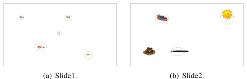
The viewers are asked to focus their attention on the four objects, one at the time. Hence, the clustering algorithms should result in four distinct clusters each pointing to one object. Examples of the ROI identification with the proposed approach overlapped with the displayed image is shown in Fig. 3. The ellipses are drawn to emphasise all samples of a cluster to make the visual clustering results clearer.

(a) Slide1. (b) Slide2.

Fig. 3. ROI estimation validation in Experiment 1 for Subject 2 with (a) words distributed, (b) icons distributed (Enlarge slightly in colour).

The comparison results between the four methods are shown in Table IV, where CD is the number of correctly detected ROIs and ID stands for the number of incorrectly detected

ROIs. Both CD and ID are averaged over all subjects. CD = 20 if all ROIs are detected correctly. An ROI is correctly detected if at least half of the samples in the resulting cluster overlap with the target object, and there are no other clusters that overlap with the target.

One can see from the table, that the proposed method leads to the highest CD and lowest ID indicating the highest ac-curacy. Generally, all methods perform well, since the objects are clear, the background is white, and the objects are far away from one another. In order to test the ROI detection accuracy in a more challenging scene, we set Experiment 2.

TABLE IV

COMPARISON OF THEROIDETECTION RESULTS BETWEEN THE PROPOSED METHOD, DB-SCAN, I-DTANDMEAN-SHIFT,FOREXPERIMENT1.CD

IS THE NUMBER OF CORRECTLY DETECTEDROIS ANDIDIS THE NUMBER OF INCORRECTLY DETECTEDROIS.

Proposed DB-SCAN I-DT Mean-shift

CD ID CD ID CD ID CD ID

Slide1 18 3 14 6 14 7 15 8

Slide2 19 2 15 5 16 7 13 6

In Experiment 2, 10 slides are shown to the subjects, all full of icons (around 70) [25]:

1) Slide1. Blank background; 2 sec on each 4 target icons. 2) Slide2. Blank background; 5 sec on each 4 target icons. 3) Slide3. Blank background and the target icons are very

small (compared to other icons in the image).

4) Slide4. Blank background and the target icons are large. 5) Slide5. Blank background; and the whole slide is noisy. 6) Slide6. Nature image as background; 2 sec on each 4

target icons.

7) Slide7. Nature image as background; 5 sec on each 4 target icons.

8) Slide8. Nature image as background and the target icons are very small.

9) Slide9. Nature image as background and the target icons are very large.

10) Slide10. Nature image as background and the whole slide is noisy.

The subjects are informed about the positions of the target icons in the slides before the experiment. During the exper-iment, the subjects are told to focus their attention on those icons. The ROI will be the target icons that the subjects are asked to focus on. The saccades while finding the target icons are noise. The numerical comparison results are shown in Table V. Figs. 4 and 5 show two examples obtained with the proposed method.

TABLE V

COMPARISON OFROIDETECTION RESULTS BETWEEN THE PROPOSED METHOD, DB-SCAN, I-DTANDMEAN-SHIFT,FOREXPERIMENT2. THE

RESULTS ARE AVERAGED OVER ALL SUBJECTS. Proposed DB-SCAN I-DT Mean-shift

CD ID CD ID CD ID CD ID

Slide1 28 1 24 12 21 5 25 5

Slide2 29 2 25 10 22 10 22 8

Slide3 26 1 20 12 18 19 20 7

Slide4 27 4 21 9 17 21 15 25

Slide5 29 2 20 5 19 6 21 3

Slide6 27 3 18 11 22 10 19 6

Slide7 30 1 20 13 21 9 19 7

Slide8 28 2 15 11 19 11 17 9

Slide9 28 3 14 10 21 7 11 23

Slide10 26 2 22 7 21 9 21 9

Mean 27.8 2.1 19.9 10 20.1 10.7 19 10.2

proposed method. As for Mean-shift, the results are relatively better than DB-SCAN and I-DT for most slides except Slides 4 and 9. The target icons in these two slides are much larger than other icons. Therefore the size of ROIs are also relative large. Mean-shift incorrectly breaks the ROI into more than one cluster.

Fig. 4. ROI estimation validation for Subject3 and Slide9.

Fig. 5. ROI estimation validation for Subject3 and Slide10.

IV. CONCLUSION

This paper proposes a spatial clustering method for ROI detection using the emerging concept of GSP. A shift prepro-cessing approach is utilised to further improve the clustering accuracy. Graph Fourier Transform is applied to evaluate the cluster quality, and thereby adjust the GSP parameter. The proposed method can provide highly accurate clustering results

on public shape clustering dataset. It also shows excellent ROI detection performance for true eye tracker data in a range of challenging scenes. Future work will consist of further improving ROI detection accuracy by adding another term in adjacency matrix definition and applying time in the graph weight to detect fixation points.

REFERENCES

[1] X. Chen and Z. Chen, “Visual attention identification using random walks based eye tracking protocols,” in2015 IEEE Global Conf. Signal and Inform. Proc. (GlobalSIP), Dec 2015, pp. 6–9.

[2] D. D. Salvucciand and J. H. Goldberg, “Identifying fixations and saccades in eye-tracking protocols,” in The 2000 ACM Symp. Eye Tracking Research & Applications, 2000, pp. 71–78.

[3] C. M. Privitera and L. W. Stark, “Algorithms for defining visual regions-of-interest: comparison with eye fixations,”IEEE Trans. Pattern Analysis and Machine Intell., vol. 22, no. 9, pp. 970–982, Sep 2000.

[4] R. O. Duda, P. E. Hart, and D. G. Stork,Pattern classification. John Wiley & Sons, 2012.

[5] M. Ester, H. Kriegel, J. Sander, and X.Xu, “A density-based algorithm for discovering clusters in large spatial databases with noise.” inKDD, vol. 96, no. 34, 1996, pp. 226–231.

[6] O. ˇSpakov and D. Miniotas, “Application of clustering algorithms in eye gaze visualizations,”Inform. Techn. and Control, vol. 36, no. 2, 2015. [7] A. Santella and D. DeCarlo, “Robust clustering of eye movement

recordings for quantification of visual interest,” inThe 2004 ACM Symp. Eye Tracking Research & Applications, 2004, pp. 27–34.

[8] A. Sandryhaila and J. M. F. Moura, “Discrete signal processing on graphs,”IEEE Trans. Signal Proc., vol. 61, pp. 1644–1656, Apr. 2013. [9] D. I. Shuman, S. K. Narang, P. Frossard, A. Ortega, and P. Van-dergheynst, “The emerging field of signal processing on graphs: Ex-tending high-dimensional data analysis to networks and other irregular domains,”IEEE Sig. Proc. Magazine, vol. 30, no. 3, pp. 83–98, 2013. [10] A. Sandryhaila and J. Moura, “Classification via regularization on

graphs.” inGlobalSIP, 2013, pp. 495–498.

[11] C. Zhang, D. Florˆencio, and P. A. Chou, “Graph signal processing– a probabilistic framework,”Microsoft Res., Redmond, WA, USA, Tech. Rep. MSR-TR-2015-31, 2015.

[12] K. He, L. Stankovic, J. Liao, and V. Stankovic, “Non-intrusive load disaggregation using graph signal processing,” IEEE Transactions on Smart Grid, to be published, 2016.

[13] C. Yang, A. Kerr, V. Stankovic, L. Stankovic, P. Rowe, and S. Cheng, “Human upper limb motion analysis for post-stroke impairment assess-ment using video analytics,”IEEE Access, vol. 4, pp. 650–659, 2016. [14] B. Zhao, L. Stankovic, and V. Stankovic, “On a training-less solution for

non-intrusive appliance load monitoring using graph signal processing,”

IEEE Access, vol. 4, pp. 1784–1799, 2016.

[15] C. Yang, Y. Mao, G. Cheung, V. Stankovic, and K. Chan, “Graph-based depth video denoising and event detection for sleep monitoring,” inIEEE Int. Workshop Multimedia Signal Proc. (MMSP), Sept 2014, pp. 1–6. [16] C. Yang, G. Cheung, V. Stankovic, K. Chan, and N. Ono, “Sleep apnea

detection via depth video and audio feature learning,” IEEE Trans. Multi., vol. 19, pp. 822–835, Apr. 2017.

[17] S.Boyd and L. Vandenberghe,Convex optimization. Cambridge uni-versity press, 2004.

[18] G. H. Golub and C. Reinsch, “Singular value decomposition and least squares solutions,”Numerische mathematik, vol. 14, pp. 403–420, 1970. [19] R. Singh, A. Chakraborty, and B. S. Manoj, “Graph fourier transform based on directed laplacian,” in2016 Int. Conf. Signal Processing and Commun. (SPCOM), June 2016, pp. 1–5.

[20] A. Sandryhaila and J. M. F. Moura, “Discrete signal processing on graphs: Frequency analysis,” IEEE Trans. Signal Processing, vol. 62, no. 12, pp. 3042–3054, June 2014.

[21] A. Sandryhaila and J. Moura, “Discrete signal processing on graphs: Graph fourier transform,” in 2013 IEEE Int. Conf. Acoustics, Speech and Signal Processing, May 2013, pp. 6167–6170.

[22] Clustering datasets. [Online]. Available: https://cs.joensuu.fi/sipu/datasets/

[23] The eye tribe. [Online]. Available: https://theeyetribe.com/

[24] OGAMA open gaze and mouse analyzer. [Online]. Available: http://www.ogama.net/