City, University of London Institutional Repository
Citation
:
Andrienko, N., Andrienko, G. & Rinzivillo, S. (2015). Exploiting spatial abstraction in predictive analytics of vehicle traffic. ISPRS International Journal of Geo-Information, 4(2), pp. 591-606. doi: 10.3390/ijgi4020591This is the published version of the paper.
This version of the publication may differ from the final published
version.
Permanent repository link:
http://openaccess.city.ac.uk/12466/Link to published version
:
http://dx.doi.org/10.3390/ijgi4020591Copyright and reuse:
City Research Online aims to make research
outputs of City, University of London available to a wider audience.
Copyright and Moral Rights remain with the author(s) and/or copyright
holders. URLs from City Research Online may be freely distributed and
linked to.
City Research Online: http://openaccess.city.ac.uk/ [email protected]
ISPRS International Journal of
Geo-Information
ISSN 2220-9964
www.mdpi.com/journal/ijgi/ Communication
Exploiting Spatial Abstraction in Predictive Analytics of
Vehicle Traffic
Natalia Andrienko 1,2,*, Gennady Andrienko 1,2,† and Salvatore Rinzivillo 3,†
1 Fraunhofer Institute IAIS, Schloss Birlinghoven, 53757 Sankt Augustin, Germany;
E-Mail: [email protected]
2 Department of Computer Science, City University London, Northamton Sqaure,
London EC1V OHB, UK; E-Mail: [email protected]
3 Istituto di Scienza e Tecnologie dell'Informazione, Consiglio Nazionale delle Ricerche,
56124 Pisa, Italy; E-Mail: [email protected]
† These authors contributed equally to this work.
This communication paper extends an unpublished discussion presentation at IEEE VIS 2014 Workshop on Visualization for Predictive Analytics, Paris, November 2014.
* Author to whom correspondence should be addressed;
E-Mail: [email protected]; Tel.: +49-2241-142486; Fax: +49-2241-142072.
Academic Editors: Jochen Schiewe and Wolfgang Kainz
Received: 2 December 2014 / Accepted: 7 April 2015 / Published: 15 April 2015
Abstract: By applying visual analytics techniques to vehicle traffic data, we found a way to visualize and study the relationships between the traffic intensity and movement speed on links of a spatially abstracted transportation network. We observed that the traffic intensities and speeds in an abstracted network are interrelated in the same way as they are in a detailed street network at the level of street segments. We developed interactive visual interfaces that support representing these interdependencies by mathematical models. To test the possibility of utilizing them for performing traffic simulations on the basis of abstracted transportation networks, we devised a prototypical simulation algorithm employing these dependency models. The algorithm is embedded in an interactive visual environment for defining traffic scenarios, running simulations, and exploring their results. Our research demonstrates a principal possibility of performing traffic simulations on the basis of spatially abstracted transportation networks using dependency models derived from real traffic data. This
possibility needs to be comprehensively investigated and tested in collaboration with transportation domain specialists.
Keywords: visual analytics; mobility; traffic modeling; traffic simulation
1. Introduction
Data concerning vehicle traffic in transportation networks are now collected in great amounts owing to advances in sensing technologies. These data offer new opportunities for improving the understanding of traffic properties and enhancing the accuracy of the models describing and forecasting traffic situations and their evolution. However, the potential of real traffic data remains largely underexploited. By means of visual analytics methods, we performed a systematic study of the hidden opportunities. We found out that traffic data covering a sufficiently long time period to reflect the regular daily and weekly variations can be used for deriving models capable of predicting not only regular traffic flows at different times but also extraordinary flows in abnormal situations, such as road closures or mass movements caused by public events or emergencies. Predicting unusual traffic behaviors on the basis of data reflecting only normal patterns becomes possible due to the reconstruction of interdependencies [1] between the traffic intensity (also known as traffic flow or flux) and the mean movement speed for different links of a transportation network.
A distinctive feature of our approach to traffic analysis, modeling, and simulation is the use of spatial abstraction for representing transportation networks and traffic properties at different spatial scales. The approach is based on the key finding that the fundamental relationships between traffic characteristics are consistent across different levels of spatial abstraction of a physical transportation network.
2. Related Works
The concept of spatial scale is one of the central concepts in the geographic sciences [2–5], where it is commonly recognized that the scale of analysis must match the actual scale of the phenomenon that is analyzed. On the other hand, the scale should also match the goals of analysis. Making justifiable choices is not easy. Often researchers use empirical trial-and-error approaches to identifying appropriate scales for analyzing phenomena. Researchers also need to check how patterns they observe change with the scale and, more generally, to address the problem of modifiable areal unit [6], which refers not only to the sizes of spatial units but also to the delineation of their boundaries. It was suggested [7] that visual analytics approaches can help spatial analysts in choosing suitable spatial and temporal scales of analysis and testing the sensitivity of findings to changes of the sizes and delineation of spatial and temporal units. This is exemplified by our research, in which interactive visual embedding of techniques for spatial abstraction and aggregation [8] facilitated the exploration of vehicle traffic at different spatial scales and, thus, enabled our key finding that fundamental relationships between traffic characteristics are consistent across multiple scales (Section 3).
parameters, and Soleymani et al. [10] suggested a framework for cross-scale analysis of movement behaviors using machine learning (classification) methods. Concerning the spatial scale, the idea is to use three hierarchical levels of space subdivision, derive various aggregate measures for the defined zones, and use these measures as features for a classification model. The scale at which the highest performance of the classifier is achieved is judged as the most appropriate. In a similar way, an appropriate temporal scale is chosen. It is not yet clear how this approach can be generalized beyond the task of movement behavior classification.
Scale is also a pertinent concept in transportation research. In particular, traffic simulation models are classified into macroscopic, mesoscopic, and microscopic [11]. Macroscopic models describe the traffic at a high level of aggregation as flow without considering individual vehicles [12,13]. In microscopic models, traffic is described at the level of individual vehicles and their interactions with each other and with the road infrastructure. Two major classes are agent-based models [14] and cellular automata models [15]. Being quite resource-demanding, microscopic models have traditionally been used for local simulations in small areas, but the increased power of computers and parallel computing have enabled microscopic simulations for large networks. A disadvantage of microscopic models is large effort required for model preparation. Mesoscopic models fill the gap between macroscopic and microscopic models by combining individual vehicle representation with aggregate representation of traffic dynamics [16]. Individual vehicles or packets of vehicles move through links of a transportation network according to general speed-density relationships defined in traffic flow theories [17] or derived from real data [18]. Parameters of these relationships can be set differently for different link types [16]. Hybrid models combine macroscopic or mesoscopic models with microscopic models [19,20]. Different model types are applied to different parts of a network. Thus, Sewall et al. [11] perform agent-based simulation of individual vehicles in regions of user’s interest while a faster macroscopic model is used in the remainder of the network.
Visualization support to traffic simulation is currently represented only by the works of Sewall et al. [11,12], who generate realistic 3D animations of simulated vehicle movements. For the hybrid micro-macro simulation, they designed an interactive tool that automatically and dynamically selects the appropriate simulation method for different parts of the network based on user’s needs. In our work, interactive visualizations and interfaces support not only traffic simulations but also analysis of real traffic data and creation of models that are subsequently applied for simulations.
3. Spatial Abstraction of a Transportation Network
Traffic data may be available in the form of trajectories of moving objects. A trajectory consists of records reporting the positions (e.g., geographic coordinates) of moving objects at different times. Given a large set of trajectories, we apply an existing method [8] that derives an abstracted network consisting of cells (territory compartments) and links between them. Smaller or larger cells can be generated by varying method parameters, thus, allowing traffic analysis and modeling at a chosen spatial scale. Moreover, it is also possible to vary the spatial scale across the territory depending on the data density and, thus, obtain finer cells in data-dense areas and coarser cells in data-sparse regions [21].
by the nodes and links of the network and temporally by time intervals [8]. The result of the aggregation includes two sets of time series for the links: traffic intensities and mean vehicle speeds (velocities). Traffic intensity on a link, also called traffic flow or flux, is the number of objects traversing the link per time unit. The mean speed on a link is computed as follows. For each object that moved from cell A to cell B, two trajectory points that are the closest to the centers of these cells are selected. Dividing the length of the path between the selected points by the time difference between them gives the mean speed of this object. The overall mean speed on the link (A,B) in a time interval [t1,t2] is computed as the mean of the mean speeds of all objects that moved from cell A to cell B during this time interval.
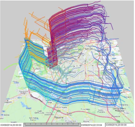
[image:5.595.51.548.325.560.2]Figure 1 gives an example of an abstracted traffic network of Milan (Italy) reconstructed from GPS tracks of 17,241 cars collected over a period of one week from Sunday, 1 April, to Saturday, 7 April, 2007 (data source: Octo Telematics SpA). The original GPS records include anonymized vehicle identifiers, time stamps, and geographic coordinates. The temporal resolution is mostly 30 seconds while larger temporal gaps also occur. In Figure 1, the territory of Milan is divided into cells with approximate radii of 1 km.
Figure 1. An abstraction of the street network of Milan (Italy) built with cell radii ≈ 1 km.
Explanation: The cells are Voronoi polygons built around the “mass centers” of spatial clusters of points extracted from the trajectories. The clustering method [8] groups the points so that each group fits in a circle of a user-specified maximal radius (1 km in our example), but the actual group radius may also be smaller. The medoid of each group (i.e., the point with the smallest sum of distances to all other points) is taken as a generating seed for Voronoi tessellation. Note that the medoid is not necessarily the center of the circumcircle of the group. The shapes and sizes of the resulting polygons depend on the spatial distribution of the group medoids. Since the latter is irregular, the cell shapes and sizes are also irregular. When we use an expression “cells with approximate radii x”, we actually mean that the cells have been built on the basis of point clusters with the maximal radius x.
representing a link increases towards the link end [22], which distinguishes the directions of the opposite links between the same cells. An alternative method for representing links is by half-arrow symbols [23], as demonstrated on the bottom right of Figure 1. It can be noted that not all pairs of neighboring cells are connected by links. The absence of a link between two cells means the absence of actual movements between these cells.
For improving the map legibility, the link symbols are colored based on results of partition-based clustering by the similarity of the associated time series of the traffic intensities and mean speeds, i.e., each color corresponds to one of the clusters. The colors for the clusters are chosen so that close clusters receive similar colors and distant clusters receive dissimilar colors. This is done by projecting the cluster centers onto a two-dimensional color space [24]. Hence, in our example, similar colors correspond to clusters of links with similar traffic intensities and mean speeds. The three clusters with the most distinctive colors (dark red, dark mauve, and violet) consist of the links located along the orbital motorway around the city and the radial motorways. The colors signify that these links differ much from the remaining links located inside the city and in the residential suburbs.
To study and quantify the relationships between the traffic intensities and mean speeds on the links, the data are transformed in the following way. Let A and B be two time-dependent attributes associated with the same object (in particular, link) and defined for the same time steps.
1. Divide the value range of attribute A into intervals. 2. For each value interval of A:
a. Find all time steps in which the values of A fit in this interval. b. Collect all values of B occurring in these time steps.
c. From the collected values of B, compute summary statistics: mean, quartiles, 9th decile (i.e., 90th percentile), and maximum.
d. For each statistical measure (i.e., mean, 9th decile, maximum, etc.), construct an ordered sequence of values corresponding to the value intervals of A arranged in the ascending order.
In this way, a family of attributes is derived: mean of B, 9th decile of B, maximum of B, and so on. For each of the derived attributes, there is an ordered sequence of values corresponding to the chosen value intervals of attribute A. This sequence is similar to a time series except that the steps are based not on time but on values of attribute A. We call such sequences dependency series (DS) since they express the dependency between attributes A and B. Attribute A is treated as the independent variable and B as the dependent variable.
To study and model the interdependencies between the mean speed and the traffic intensity, we perform two transformations. First, we treat the traffic intensity as the independent variable and derive a family of attributes expressing the dependency of the mean speed on the traffic intensity. Second, we treat the mean speed as the independent variable and derive a family of attributes expressing the dependency of the traffic intensity on the mean speed. Dependency series may be derived using either the absolute or relative traffic intensities, the latter being computed as the ratios or percentages of the absolute intensities to the maximal intensities attained on the same links.
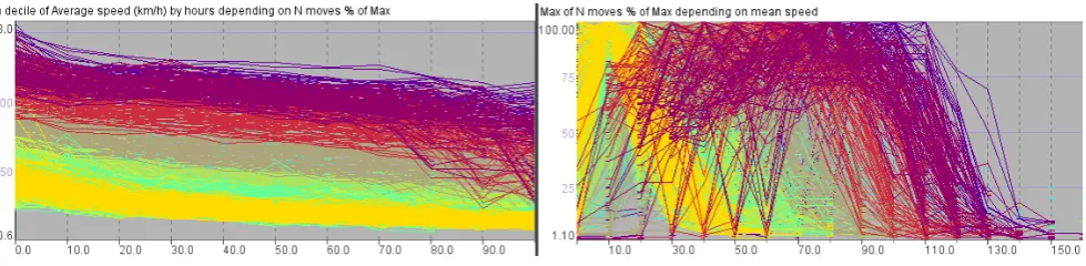
Figure 1. The graph on the left shows how the mean speed depends on the relative traffic intensity expressed as the percentage to the maximum. The horizontal axis corresponds to the traffic intensity and the vertical axis to the 9th decile of the mean speed. We have taken the 9th decile because this statistical measure is less sensitive to outliers as the maximum. Outliers among the values of the mean speed often occur in time intervals of low traffic intensity, when a single or only a few vehicles traverse a link. The graph on the right shows for each link the dependency of the maximal relative traffic intensity on the mean speed. The horizontal axis corresponds to the mean speed and the vertical axis to the maximal relative traffic intensity.
Figure 2. The graphs represent the interdependencies between the traffic intensity and mean speed for the links of the abstracted transportation network of Milan shown in Figure 1.
On the left of Figure 2, the shapes of the lines show that the mean speed decreases with increasing traffic intensity. On the right, the lines have the shape of a bell or symbol “⌒”, which can be interpreted as follows. When vehicles move with a low mean speed, only a small number of vehicles can traverse a link in a time unit, i.e., the traffic intensity is low. When the mean speed increases, the intensity also increases, but only till the point when a certain “optimal” value of the mean speed is reached. After this point, movement with higher mean speeds is only possible when the traffic intensity decreases. These observations conform to our commonsense knowledge and experiences concerning the behavior of the vehicle traffic on roads but refer to an abstracted rather than physical transportation network.
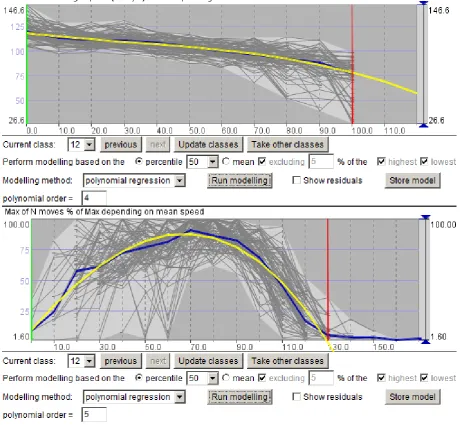
Figure 3. The two-way dependencies between the traffic intensity and mean speed can be represented by polynomial regression models.
The fundamental diagram refers to links of a physical transportation network, i.e., to street segments. The exact parameters of the curves depend on the street properties, such as the width, number of lanes, and speed limit. We see that the same relationships as in a physical network exist also in a spatially abstracted network. The parameters of the curves depend on the properties of the abstracted links. As each abstracted link stands for a group of physical links, its properties incorporate and summarize the properties of these physical links. Moreover, we have found that the relationships conforming to the fundamental traffic diagram exist on different levels of spatial abstraction, as illustrated in Figure 4.
Figure 4. The maps show spatially abstracted transportation networks of Milan built with cell radii ≈ 2 km (top) and 4 km (bottom). The graphs to the right of each map represent the two-way dependencies between the relative traffic intensities and the mean speeds on the network links.
We have checked this finding using a much larger dataset covering the geographical region of Tuscany (Italy) and a time period of one month. Similar relationships as in Milan have been observed at diverse spatial scales for traffic flows both within and between the towns of Tuscany.
are commonly used for traffic flow prediction and simulation, which is usually done on the basis of a physical street network. The existence of similar relationships at higher levels of spatial abstraction makes it possible to do modeling, prediction, and simulation also at higher spatial scales in cases when fine details are not necessary.
4. Advantages and Limitations of Spatial Abstraction
Spatial abstraction of a street network offers following advantages:
1. The number of nodes and links in an abstracted network can be much smaller than in the underlying physical network. Hence, much less time and effort is needed for model building and calibration, and also simulations can be carried out much faster compared to the current practices. This enables, in particular, rapid approximate predictions and assessments of traffic dynamics in emergency situations, when time is very limited.
2. Spatial abstraction compensates for the sparseness of real data on streets with low traffic. There may be not enough trajectory points on a given street segment for reconstructing the dependency between the mean speed and traffic intensity, but aggregation of several physical links into one abstract link alleviates this problem.
3. It is possible to build an abstract network in which the level of spatial abstraction varies across a territory according to the variation of the data density. In areas with high traffic, abstracted links may very closely approximate physical links (i.e., street segments), whereas areas with low traffic can be represented by large cells. Hence, it is possible to have different levels of detail in traffic simulations and prediction in areas with high and low traffic, when fine details in low traffic areas are not important.
We do not claim that the spatial scale (i.e., the cell sizes) can be unlimitedly increased without distorting and eventually destroying the shapes of the curves representing the relationships between the traffic fluxes and velocities. Generally, increasing the spatial scale increases the amount of noise (i.e., oscillations) within the curves. The overall shapes of the curves remain discernible up to a certain abstraction level, at which the oscillations become too high. Our experiments show that the upper limit for the cell sizes may depend on the number and diversity of the existing physical links between the cells. Thus, for Milan and the urban areas of Tuscany, increasing the cell radius beyond 4 km distorts the curves too much, whereas much larger cells can be used for the rural areas of Tuscany. Hence, there is no uniform upper limit to the level of spatial abstraction that would be valid everywhere. An appropriate level for a given territory and available data can be determined empirically with the use of visual analytics techniques.
the simplification of the reality that makes models practically useful. The reality is so complex that, even if it would be possible to build a model representing some part of it in its full detail, this model would be intractable. In transportation, each class of models (macroscopic, mesoscopic, microscopic, or hybrid) simplifies the reality in its specific way. It would not be valid to say that some ways are better than others; rather, the different ways are suitable for different purposes. We propose a yet another approach to simplification, which is not supposed to replace any of the existing approaches but can complement them. The possible use cases for it are listed at the beginning of the section. We discussed our approach with transportation researchers from the University of Hasselt (Belgium), with whom we collaborated in a research project. They find the approach sensible and promising while requiring further substantiation by additional empirical studies.
5. Deriving Traffic Models from Real Data
A reservation needs to be made concerning the reconstruction of the fundamental relationships between the traffic flow characteristics from real vehicle trajectories. It is typical that available trajectories cover only a sample of vehicles that move within a network and not the entire population. Hence, the traffic intensities computed from these trajectories need to be appropriately scaled, to approximate the real intensities. This reservation is not specific to spatially abstracted networks but also applies to detailed street networks. Appropriate scaling parameters (or even scaling functions capturing daily and weekly variations) can be derived by comparing the vehicle counts computed from trajectory data with measured counts obtained from traffic sensors [25].
For model derivation, we apply a methodology [24] in which an interactive visual interface to a modeling library is utilized. The methodology is applicable to aggregated movement data associated with nodes and links of a network, which may be a physical street network or a spatially abstracted network. The data must include time series of the traffic intensities, that is, the counts of objects that moved through the links by time intervals, and time series of the corresponding mean speeds of their movement. The length and temporal resolution of the time series must be suitable for capturing the traffic variation related to the daily and weekly temporal cycles, which means that the length must be at least one week (more is better) and the resolution must be at most one hour (finer is better). Ideally, the counts should represent the entire population of the objects that moved over the network, but it is also possible to use data obtained for a large sample of objects after applying appropriate scaling.
dependencies between the traffic intensity and mean speed is described in more detail in a recently published book [21].
Since the models are derived for link clusters, each model by itself makes a common prediction for all cluster members. However, this prediction is individually adjusted for each cluster member based on the statistics of the distribution of its original values [24].
6. Use of Models for Traffic Prediction and Simulation
The models of the temporal variation of the traffic intensity can be used for prediction of the regular traffic for chosen time intervals in the future, assuming that the properties of the temporal variation do not change. When real traffic data are collected on a regular basis, it is reasonable to periodically check the models against the real data. If the prediction quality degrades, the models need to be updated.
The models of the dependencies between the traffic intensity and the mean speed can be used to simulate and predict unusual traffic behaviors. The main idea is following:
1. For each link, determine how many vehicles need to move through it in the current minute. 2. Using the dependency model from the traffic intensity to the mean speed, determine the mean speed that is possible for this link load.
3. Using the dependency model from the mean speed to the traffic intensity, determine how many vehicles will actually be able to move through the link in this minute.
4. Promote this number of vehicles to the end place of the link and suspend the remaining vehicles in the start place of the link.
To perform a simulation, the analyst needs to define the scenario to be simulated. This includes defining a set of extra vehicles that will be moving in the network in addition to the regular traffic, the origins and destinations of their trips, the routes they will follow, and the time when each vehicle starts moving. To support the process of scenario definition, we have developed a wizard guiding the analyst through the required steps and providing visual feedback at each step. However, the description of the wizard and the other interactive visual tools that are used is out of the scope of this paper, the objective of which is to present the key idea and outline the approach that is based on this idea. Therefore, we give only a brief example of how the simulation can be used.
For Milan, we have performed experiments on simulating the movement of a large number of personal cars from the area around the San Siro stadium after a soccer game. To be able to simulate this scenario, we need to solve the problem of data scaling mentioned at the end of Section 2. The data that we used for model building represent not all vehicles that moved in Milan but only about 2% of the private cars. We apply the following approach. If we need to simulate movements of N private cars, we downscale this number to 2% of N, to make it compatible with the models. Figures 5 and 6 present simulated trajectories of 250 cars, which correspond to about 12,500 cars in the real scale.
Figure 5. Simulated trajectories of cars moving from the vicinity of the San Siro stadium to supposed home places after a soccer game are shown in a space-time cube.
probability of choosing a cell is proportional to the cell weight, which is the sum of the hourly counts of trip ends in the hours from 6:00 p.m. to 12:00 a.m.
Figure 6. The simulated trajectories are shown on a map. The red and green circles represent the trip origins and destinations, respectively.
Besides viewing the simulated trajectories in a space-time cube and on a map, which may be animated for showing the car movements over time, there are further opportunities for analysis. The tool aggregates the simulation results for the cells and links by time intervals of user-chosen length. Using time graph displays, we can analyze the link loads, attained mean speeds, and numbers of suspended cars in the cells. Bottlenecks in the transportation infrastructure can be revealed.
After analyzing the predicted development of the traffic situation, it is possible to introduce modifications in the scenario (e.g., disable the use of some links and/or modify link weights, to model traffic re-routing) and run a new simulation. Through such “what if” analysis, it may be possible to find suitable measures for decreasing traffic suspensions and congestions.
7. Evaluation of Model Goodness
the real data. The analyst selects a quiet time interval tq and a busy time interval tb and finds the difference ΔN between the total numbers of the vehicles N(tb) and N(tq) that were present in the network in these two intervals: ΔN = N(tb) − N(tq). Then the analyst simulates the scenario as if ΔN extra vehicles appeared in the network in the time interval tq in addition to the normal traffic for tq. The extra vehicles are distributed over the nodes of the network proportionally to the differences in the vehicle counts between the intervals tb and tq. After performing the simulation, the predicted traffic intensities combining the regular and extra traffic are compared with the real traffic intensities in the interval tb. The evaluation is repeated several times for different pairs of tq and tb. We applied this approach to the models built for Milan and for Tuscany and obtained very high correlations between the predicted and real values.
8. Conclusion
In the recent years, our research was strongly focused on analysis of data concerning movement [21], including network-constrained movement. By developing and applying various visual analytics methods, we strived at comprehensive exploration of the potential opportunities that can be provided by movement data. For network-constrained movement, we found data transformations that allowed us to visualize the interdependencies between two key aspects of the movement, traffic intensity and speed. Having vivid pictures, as in Figures 2 and 4, we noticed common patterns and got an idea that the interdependencies can be quantified and expressed formally in a uniform way. To implement this idea, we developed additional visual analytics tools that enabled us to represent the dependencies by formal models. This shows that visual analytics methods can help analysts not only to gain understanding (i.e., a mental model) of a phenomenon represented by data, but also to transform this mental model into explicit formal models.
Our next idea was that the models capturing the traffic intensity—speed relationships can allow prediction of not only typical movements but also unusual movements that were not represented in the original data. This is possible because the models generalize the data and can extrapolate beyond the original scope of the data. We have developed a traffic simulation tool capable of using the models derived from real traffic data and a visual analytics infrastructure that supports definition of traffic scenarios to simulate and analysis of simulation results.
Our research showed a principal possibility of using knowledge gained from real movement data for prediction of development of traffic situations, even under unusual conditions. Moreover, one of our findings was that the dependencies between the traffic intensity and speed existing in a spatially abstracted network are similar to the known dependencies existing in road traffic and observed at the level of road segments. This opens a potential opportunity for performing rapid large-scale simulations of traffic situation developments on large territories when fine details are not required. This opportunity needs to be comprehensively investigated and tested in collaboration with transportation domain specialists.
Acknowledgments
Author Contributions
All authors contributed equally to this work.
Conflicts of Interest
The authors declare no conflict of interest.
References
1. Gazis, D.C. Traffic Theory; Kliwer Academic: Boston, MA, USA, 2002.
2. Hudson, J.C. Scale in space and time. In Geography’s Inner Worlds: Pervasive Themes in
Contemporary American Geography; Abler, R.F., Marcus, M.G., Olson, J.M., Eds.; Rutgers University Press: New Brunswick, NJ, USA, 1992; pp. 280–297.
3. Goodchild, M.F. Models of scale and scales of modelling. In Modelling Scale in Geographical
Information Science; Tate, N.J., Atkinson, P.M., Eds.; John Wiley & Sons, Ltd.: Chichester, UK, 2001; pp. 3–10.
4. Mackaness, W.A. Understanding geographic space. In Generalisation of Geographic Information: Cartographic Modelling and Applications; Mackaness, W.A., Ruas, A., Sarjakoski, T., Eds.; Elsevier: Oxford, UK, 2007; pp. 1–10.
5. Lloyd, C.D. Exploring Spatial Scale in Geography; Wiley-Blackwell: Chichester, UK, 2014; p. 253.
6. Openshaw, S. The Modifiable Areal Unit Problem; Geo Books: Norwich, UK, 1984.
7. Andrienko, G.; Andrienko, N.; Demšar, U.; Dransch, D.; Dykes, J.; Fabrikant, S.; Jern, M.;
Kraak, M.-J.; Schumann, H.; Tominski, C. Space, time, and visual analytics. Int. J. Geogr. Inf. Sci.
2010, 24, 1577–1600.
8. Andrienko, N.; Andrienko, G. Spatial generalization and aggregation of massive movement data.
IEEE Trans. Vis. Comput. Gr.2011, 17, 205–219,
9. Laube, P.; Purves, R. How fast is a cow? Cross-scale analysis of movement data. Trans. GIS2011, 15, 401–418.
10. Soleymani, A.; Cachat, J.; Robinson, K.; Dodge, S.; Kalueff, A.; Weibel, R. Integrating cross-scale analysis in the spatial and temporal domains for classification of behavioral movement. J. Spat. Inf. Sci. (JOSIS), 2014, 8, 1–25.
11. Sewall, J.; Wilkie, D.; Lin, M.C. Interactive hybrid simulation of large-scale traffic. ACM Trans. Gr.2011, 30, doi:10.1145/2024156.2024169.
12. Sewall, J.; Wilkie, D.; Merrell, P.; Lin, M.C. Continuum traffic simulation. Comput. Gr. Forum
2010, 29, 439–448.
13. Lighthill, M.H.; Whitham, G.B. On Kinematic waves II: A theory of traffic flow on long crowded roads. Proc. R. Soc. Lond. A2291955, 1178, 317–345.
14. Newell, G. Nonlinear effects in the dynamics of car following. Oper. Res.1961, 9, 209–229. 15. Nagel, K.; Schreckenberg, M. A cellular automaton model for freeway traffic. J. Phys. I 1992, 2,
16. Burghout, W.; Koutsopoulos, H.N.; Andreasson, I. A discrete-event mesoscopic traffic simulation model for hybrid traffic simulation. In Proceedings of the 2006 IEEE Intelligent Transportation Systems Conference (ITSC’06), Toronto, ON, Canada, 17–20 September 2006; pp. 1102–1107. 17. DelCastillo, J.M.; Benitez, F.G. On the functional form of the speed-density relationship I: General
theory. Transp. Res. Part B: Methodol.1995, 29, 373–389.
18. Helbing, D. Derivation of a fundamental diagram for urban traffic flow. Eur. Phys. J. B2009, 70, 229–241.
19. Bourrel, E.; Lesort, J.-B. Mixing micro and macro representations of traffic flow: A hybrid model based on the LWR theory. In Proceedings of the 82th Annual Meeting of the Transportation Research Board, Washington, DC, USA, 12 January 2003.
20. Burghout, W.; Koutsopoulos, H.N.; Andreasson, I. Hybrid mesoscopic-microscopic traffic
simulation. Transp. Res. Rec.2005, 1034, 218–225.
21. Andrienko, G.; Andrienko, N.; Bak, P.; Keim, D.; Wrobel, S. Visual Analytics of Movement;
Springer: Heidelberg, Germany, 2013.
22. Wood, J.; Slingsby, A.; Dykes, J. Visualizing the dynamics of London’s bicycle hire scheme.
Cartographica2011, 46, 239–251.
23. Tobler, W. Experiments in migration mapping by computer. Am. Cartogr.1987, 14, 155–163.
24. Andrienko, N.; Andrienko, G. A visual analytics framework for spatio-temporal analysis and
modeling. Data Min. Knowl. Discov.2013, 27, 55–83.
25. Pappalardo, L.; Rinzivillo, S.; Qu, Z.; Pedreschi, D.; Giannotti, F. Understanding the patterns of car travel. Eur. Phys. J. Spec. Top.2013, 215, 61–73.
26. Giannotti, F.; Nanni, M.; Pedreschi, D.; Pinelli, F.; Renso, C.; Rinzivillo, S.; Trasarti, R. Unveiling the complexity of human mobility by querying and mining massive trajectory data. VLDB J.2011, 20, 695–719.