BHA PV scheme analysis
Report produced by University of Strathclyde for the Accelerating Renewables
Connection Project
Authors:
Milana Plecas: [email protected]
Ivana Kockar: [email protected]
Contributions from:
Andrew Park, Martin Wright
Date of Issue: 15
thJune 2016
Contents
List of Tables ...6
List of Figures ...8
1 Introduction ... 10
2 Berwickshire Housing Association’s solar scheme ... 11
3 Monitoring and modelling ... 15
3.1 Monitoring equipment ... 15
3.2 Modelling ... 17
4 Methodology, analysis and results ... 20
4.1 Dovecote ... 23
4.2 Gunsgreenhill ... 24
4.3 Dulcecraig ... 25
4.4 Hoprig Road ... 26
4.5 Swinton Duns ... 27
4.6 Chirnside West End ... 28
4.7 Ayton Lawfield ... 29
4.8 Briery Baulk ... 29
4.9 Buss Craig ... 30
4.10 Castle Street... 30
4.11 Churchill ... 30
4.12 Deanhead ... 31
4.13 Grantshouse ... 31
4.14 Hawthorn Bank Duns ... 32
4.15 Leitholm Village ... 32
5 Conclusions and next steps ... 33
Appendix 1 Cable types ... 34
A 1.1 11kV Cables and Overhead Lines ... 35
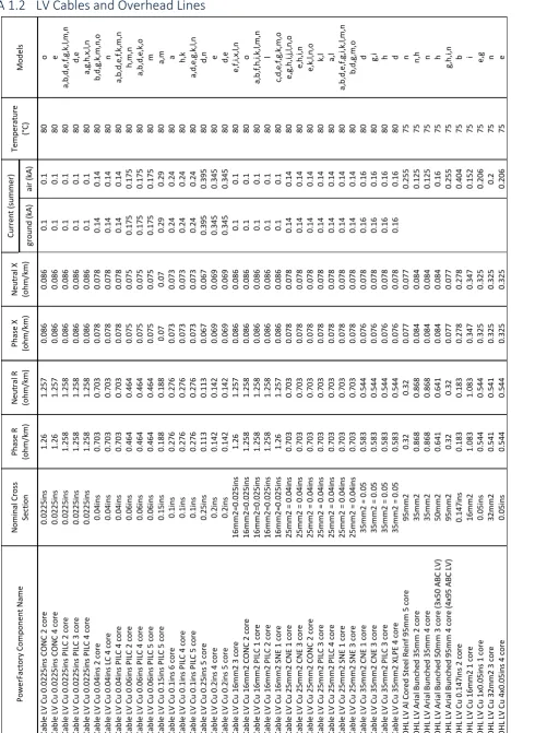
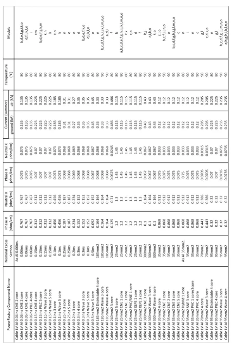
A 1.2 LV Cables and Overhead Lines ... 36
Appendix 2 Description of the models ... 38
A 2.1 Ayton Lawfield ... 38
A 2.1.1 11kV model ... 38
A 2.1.2 LV model ... 40
A 2.2 Briery Baulk ... 42
A 2.2.1 11kV model ... 42
A 2.2.2 LV model ... 43
A 2.3.2 LV model ... 46
A 2.4 Castle Street ... 48
A 2.4.1 11kV model ... 48
A 2.4.2 LV model ... 49
A 2.5 Churchill ... 52
A 2.5.1 11kV model ... 52
A 2.5.2 LV model ... 53
A 2.6 Deanhead ... 55
A 2.6.1 11kV model ... 55
A 2.6.2 LV model ... 56
A 2.7 Dovecote ... 58
A 2.7.1 11kV model ... 58
A 2.7.2 LV model ... 59
A 2.8 Dulcecraig ... 61
A 2.8.1 11kV model ... 61
A 2.8.2 LV model ... 62
A 2.9 Grantshouse ... 64
A 2.9.1 11kV model ... 64
A 2.9.2 LV model ... 65
A 2.10 Gunsgreenhill ... 68
A 2.10.1 11kV model ... 68
A 2.10.2 LV model ... 69
A 2.11 Hawthorn Bank Duns ... 71
A 2.11.1 11kV model ... 71
A 2.11.2 LV model ... 72
A 2.12 Hoprig Road ... 74
A 2.12.1 11kV model ... 74
A 2.12.2 LV model ... 76
A 2.13 Leitholm Village ... 78
A 2.13.1 11kV model ... 78
A 2.13.2 LV model ... 79
A 2.14 Swinton Duns ... 81
A 2.14.1 11kV model ... 81
A 2.14.2 LV model ... 82
A 2.15 Chirnside West End ... 84
A 2.15.2 LV model ... 85
Appendix 3 PV systems included in the models ... 87
A 3.1 Ayton Lawfield ... 87
A 3.2 Briery Baulk ... 88
A 3.3 Buss Craig ... 88
A 3.4 Castle Street ... 89
A 3.5 Churchill ... 89
A 3.6 Deanhead ... 90
A 3.7 Dovecote ... 91
A 3.8 Dulcecraig ... 92
A 3.9 Grantshouse ... 93
A 3.10 Hawthorn Bank Duns ... 93
A 3.11 Gunsgreenhill ... 94
A 3.12 Hoprig Road ... 95
A 3.13 Leitholm Village ... 96
A 3.14 Swinton Duns ... 96
A 3.15 Chirnside West End ... 97
Appendix 4 Loads included in the models ... 98
A 4.1 Ayton Lawfield ... 99
A 4.2 Briery Baulk ... 100
A 4.3 Buss Craig ... 101
A 4.4 Castle Street ... 102
A 4.5 Churchill ... 103
A 4.6 Deanhead ... 104
A 4.7 Dovecote ... 106
A 4.8 Dulcecraig ... 107
A 4.9 Grantshouse ... 108
A 4.10 Hawthorn Bank Duns ... 109
A 4.11 Gunsgreenhill ... 110
A 4.12 Hoprig Road ... 111
A 4.13 Leitholm Village ... 112
A 4.14 Swinton Duns ... 113
List of Tables
Table 1: Transformer rating, numbers of LV feeders, customers and PVs at each modelled S/S ... 17
Table 2: Summary of developed methodologies based on their input data ... 21
Table 3: Results at Dovecote S/S for winter period in 2015 ... 23
Table 4: Results at Dovecote S/S for predicted summer loads in 2015 and 100% of PV output ... 23
Table 5: Results at Dovecote S/S for predicted summer loads in 2015 and 85% of PV output ... 23
Table 6: Results at Dovecote S/S for summer period in 2015 ... 24
Table 7: Results at Gunsgreenhill S/S for winter period in 2015 ... 24
Table 8: Results at Gunsgreenhill S/S for predicted summer loads in 2015 and 100% of PV output ... 24
Table 9: Results at Gunsgreenhill S/S for predicted summer loads in 2015 and 85% of PV output ... 24
Table 10: Results at Dulcecraig S/S for winter period in 2015 ... 25
Table 11: Results at Dulcecraig S/S for predicted summer loads in 2015 and 100% of PV output ... 25
Table 12: Results at Dulcecraig S/S for predicted summer loads in 2015 and 85% of PV output ... 25
Table 13: Results at Dulcecraig S/S for summer period in 2015 ... 26
Table 14: Results at Hoprig Road S/S for winter period in 2015 ... 26
Table 15: Results at Hoprig Road S/S for predicted summer loads in 2015 and 100% of PV output ... 26
Table 16: Results at Hoprig Road S/S for predicted summer loads in 2015 and 85% of PV output ... 26
Table 17: Results at Swinton Duns S/S for winter period in 2015 ... 27
Table 18: Results at Swinton Duns S/S for predicted summer loads in 2015 and 100% of PV output ... 27
Table 19: Results at Swinton Duns S/S for predicted summer loads in 2015 and 85% of PV output ... 27
Table 20: Results at Swinton Duns S/S for summer period in 2015 ... 28
Table 21: Results at Chirnside West End S/S for winter period in 2015 ... 28
Table 22: Results at Chirnside West End S/S for predicted summer loads in 2015 and 100% of PV output ... 28
Table 23: Results at Chirnside West End S/S for predicted summer loads in 2015 and 85% of PV output ... 28
Table 24: Results at Chirnside West End S/S for summer period in 2015 ... 29
Table 25: Results at Ayton Lawfield S/S for summer period in 2015 ... 29
Table 26: Results at Briery Baulk S/S for summer period in 2015 ... 30
Table 27: Results at Buss Craig S/S for summer period in 2015 ... 30
Table 28: Results at Castle Street S/S for summer period in 2015 ... 30
Table 29: Results at Churchill S/S for summer period in 2015 ... 31
Table 30: Results at Deanhead S/S for summer period in 2015 ... 31
Table 31: Results at Grantshouse S/S for summer period in 2015 ... 32
Table 32: Results at Hawthorn Bank Duns S/S for summer period in 2015 ... 32
Table 33: Results at Leitholm Village S/S for summer period in 2015 ... 32
Table 34: 11kV cables and overhead lines ... 35
Table 35: LV Copper cables and overhead lines ... 36
Table 36: LV Aluminium cables ... 37
Table 37: Summary of secondary substations included in 11kV Ayton Lawfield PowerFactory model ... 39
Table 38: Summary of LV loads and PV systems included in Ayton Lawfield LV PowerFactory model ... 40
Table 39: Summary of secondary substations included in 11kV Briery Baulk PowerFactory model ... 42
Table 40: Summary of LV loads and PV systems included in Briery Baulk LV PowerFactory model ... 44
Table 41: Summary of secondary substations included in 11kV Buss Craig PowerFactory model ... 45
Table 42: Summary of LV loads and PV systems included in Buss Craig LV PowerFactory model ... 46
Table 43: Summary of secondary substations included in 11kV Castle Street PowerFactory model ... 49
Table 44: Summary of LV loads and PV systems included in Castle Street LV PowerFactory model ... 50
Table 45: Summary of secondary substations included in 11kV Churchill PowerFactory model ... 52
Table 46: Summary of LV loads and PV systems included in Churchill LV PowerFactory model ... 53
Table 48: Summary of LV loads and PV systems included in Deanhead LV PowerFactory model ... 56
Table 49: Summary of secondary substations included in 11kV Dovecote PowerFactory model ... 58
Table 50: Summary of LV loads and PV systems included in Dovecote LV PowerFactory model ... 59
Table 51: Summary of secondary substations included in 11kV Dulcecraig PowerFactory model ... 61
Table 52: Summary of LV loads and PV systems included in Dulcecraig LV PowerFactory model ... 62
Table 53: Summary of secondary substations included in 11kV Grantshouse PowerFactory model ... 65
Table 54: Summary of LV loads and PV systems included in Grantshouse LV PowerFactory model ... 66
Table 55: Summary of secondary substations included in 11kV Gunsgreenhill PowerFactory model ... 68
Table 56: Summary of LV loads and PV systems included in Gunsgreenhill LV PowerFactory model ... 69
Table 57: Summary of secondary substations included in 11kV Hawthorn Bank Duns PowerFactory model ... 71
Table 58: Summary of LV loads and PV systems included in Hawthorn Bank Duns LV PowerFactory model .... 72
Table 59: Summary of secondary substations included in 11kV Hoprig Road PowerFactory model ... 75
Table 60: Summary of LV loads and PV systems included in Hoprig Road LV PowerFactory model ... 76
Table 61: Summary of secondary substations included in 11kV Leitholm Village PowerFactory model ... 79
Table 62: Summary of LV loads and PV systems included in Leitholm Village LV PowerFactory model ... 80
Table 63: Summary of secondary substations included in 11kV Swinton Duns PowerFactory model ... 81
Table 64: Summary of LV loads and PV systems included in Swinton Duns LV PowerFactory model ... 83
Table 65: Summary of secondary substations included in 11kV Chirnside West End PowerFactory model ... 84
Table 66: Summary of LV loads and PV systems included in Chirnside West End LV PowerFactory model ... 86
Table 67: Proposed PVs at Ayton Lawfield S/S ... 87
Table 68: Proposed PVs at Briery Baulk S/S... 88
Table 69: Proposed PVs at Buss Craig S/S ... 88
Table 70: Proposed PVs at Castle Street S/S ... 89
Table 71: Proposed PVs at Churchill S/S ... 89
Table 72: Proposed PVs at Deanhead S/S ... 90
Table 73: Proposed PVs at Dovecote S/S... 91
Table 74: Proposed PVs at Dulcecraig S/S ... 92
Table 75: Proposed PVs at Grantshouse S/S ... 93
Table 76: Proposed PVs at Hawthorn Bunk Duns S/S ... 93
Table 77: Proposed PVs at Gungreenhill S/S ... 94
Table 78: Proposed PVs at Hoprig Road S/S ... 95
Table 79: Proposed PVs at Leitholm Village S/S ... 96
Table 80: Proposed PVs at Swinton Duns S/S ... 96
Table 81: Proposed PVs at Chirnside West End S/S ... 97
Table 82: Loads connected to Ayton Lawfield S/S ... 99
Table 83: Loads connected to Briery Baulk S/S ... 100
Table 84: Loads connected to Buss Craig S/S ... 101
Table 85: Loads connected to Castle Street S/S ... 102
Table 86: Loads connected to Chirchill S/S ... 103
Table 87: Loads connected to Deanhead S/S ... 105
Table 88: Loads connected to Dovecote S/S ... 106
Table 89: Loads connected to Dulcecraig S/S ... 107
Table 90: Loads connected to Grantshouse S/S ... 108
Table 91: Loads connected to Hawthorn Bank Duns S/S ... 109
Table 92: Loads connected to Gunsgreenhill S/S ... 110
Table 93: Loads connected to Hoprig Road S/S ... 111
Table 94: Loads connected to Leitholm Village S/S ... 112
Table 95: Loads connected to Swinton Duns S/S ... 113
List of Figures
Figure 1: The ARC trial area and an area proposed for BHA PV installations ... 11
Figure 2: Number of PV approved properties aggregated to Grid Supply Points ... 12
Figure 3: Number of PV approved properties aggregated to primary substations ... 12
Figure 4: Example of PV approved properties at a single secondary substation ... 13
Figure 5: Installed PV panels ... 13
Figure 6: The flowchart of the analysis... 14
Figure 7: Overview of monitored secondary substations ... 15
Figure 8: Monitored secondary substations ... 16
Figure 9: GMC-I METSyS substation monitor ... 16
Figure 10: Gridkey MCU 520 susbstation monitor ... 17
Figure 11: Example of SPEN's GIS system displaying a single substation with LV feeder cables and services ... 18
Figure 12: PowerFactory example of a single secondary substation with its respective 11kV circuits ... 19
Figure 13: PowerFactory example of a single secondary substation with its respective LV feeders. This is the same area of SPEN’s network as shown in Figure 11. ... 19
Figure 14: PowerFactory model of 11kV circuit 120/22 provided by SPEN ... 38
Figure 15: Ayton Lawfield 11kV PowerFactory model ... 39
Figure 16: Ayton Lawfield LV PowerFactory model indicating LV feeders ... 40
Figure 17: Ayton Lawfield LV PowerFactory model indicating LV phasing ... 41
Figure 18: PowerFactory model of 11kV circuit 114/24 provided by SPEN ... 42
Figure 19: Briery Baulk 11kV PowerFactory model ... 43
Figure 20: Briery Baulk LV PowerFactory model indicating LV feeders ... 43
Figure 21: Briery Baulk LV PowerFactory model indicating LV phasing ... 44
Figure 22: Buss Craig 11kV PowerFactory model ... 45
Figure 23: Buss Craig LV PowerFactory model indicating LV feeders... 46
Figure 24: Buss Craig LV PowerFactory model indicating LV phasing ... 47
Figure 25: PowerFactory model of 11kV circuit 114/22 provided by SPEN ... 48
Figure 26: Castle Street 11kV PowerFactory model ... 49
Figure 27: Castle Street LV PowerFactory model indicating LV feeders ... 50
Figure 28: Castle Street LV PowerFactory model indicating LV phasing ... 51
Figure 29: Churchill 11kV PowerFactory model ... 52
Figure 30: Churchill LV PowerFactory model indicating LV feeders ... 53
Figure 31: Churchill LV PowerFactory model indicating LV phasing ... 54
Figure 32: Deanhead 11kV PowerFactory model ... 55
Figure 33: Deanhead LV PowerFactory model indicating LV feeders ... 56
Figure 34: Deanhead LV PowerFactory model indicating LV phasing ... 57
Figure 35: Dovecote 11kV PowerFactory model ... 58
Figure 36: Dovecote LV PowerFactory model indicating LV feeders ... 59
Figure 37: Dovecote LV PowerFactory model indicating LV phasing ... 60
Figure 38: Dulcecraig 11kV PowerFactory model ... 61
Figure 39: Dulcecraig LV PowerFactory model indicating LV feeders ... 62
Figure 40: Dulcecraig LV PowerFactory model indicating LV phasing ... 63
Figure 41: PowerFactory model of 11kV circuit 120/21 provided by SPEN ... 64
Figure 42: Grantshouse 11kV PowerFactory model ... 65
Figure 43: Grantshouse LV PowerFactory model indicating LV feeders ... 66
Figure 44: Grantshouse LV PowerFactory model indicating LV phasing ... 67
Figure 45: Gunsgreenhill 11kV PowerFactory model ... 68
Figure 47: Gunsgreenhill LV PowerFactory model indicating LV phasing ... 70
Figure 48: Hawthorn Bank Duns 11kV PowerFactory model ... 71
Figure 49: Hawthorn Bank Duns LV PowerFactory model indicating LV feeders ... 72
Figure 50: Hawthorn Bank Duns LV PowerFactory model indicating LV phasing ... 73
Figure 51: PowerFactory model of 11kV circuit 344/24 provided by SPEN ... 74
Figure 52: Hoprig Road 11kV PowerFactory model ... 75
Figure 53: Hoprig Road LV PowerFactory model indicating LV feeders ... 76
Figure 54: Hoprig Road LV PowerFactory model indicating LV phasing ... 77
Figure 55: PowerFactory model of 11kV circuit 114/23 provided by SPEN ... 78
Figure 56: Leitholm Village 11kV PowerFactory model ... 79
Figure 57: Leitholm Village LV PowerFactory model indicating LV feeders ... 79
Figure 58: Leitholm Village LV PowerFactory model indicating LV phasing ... 80
Figure 59: PowerFactory model of 11kV circuit 118/14 provided by SPEN ... 81
Figure 60: Swinton Duns 11kV PowerFactory model ... 82
Figure 61: Swinton Duns LV PowerFactory model indicating LV feeders ... 82
Figure 62: Swinton Duns LV PowerFactory model indicating LV phasing ... 83
Figure 63: PowerFactory model of 11kV circuit 121/22 provided by SPEN ... 84
Figure 64: Chirnside West End 11kV PowerFactory model ... 85
Figure 65: Chirnside West End LV PowerFactory model indicating LV feeders ... 85
1
Introduction
Small-scale distributed generation (DG), such as photovoltaic (PV) panels, are normally connected to the Low Voltage (LV) network. Small numbers of DGs does not usually cause any significant negative impact on the local LV network. However, significant network issues are possible when their penetration levels are high. This could result in bi-directional power flows and thermal overloading as well as voltage rise and phase imbalance.
SP Energy Networks (SPEN) manages connections at the LV network level according to either ER G59/3 or ER G83/21. The former covers DG connections above 16A and the latter covers small-scale DG connections (up to
16A per phase).
Applications for single small-scale DG installations, up to the limit of 16A per phase, are covered under G83 Stage 1. In this case, there is no need for network changes and the installer is required to inform the Distribution Network Operator (DNO) within 28 days that the unit is installed and commissioned. The DNO then records the unit location and capacity on their GIS system.
On the other hand, multiple installations, for example multiple applications from a Housing Association, require a consent from the DNO before they can connect. After the developer submits an application under G83/2 Stage 2, a generation assessment by the DNO is required in order to ensure that the cumulative effect of multiple connections will not cause the distribution network to operate outside its design limits. These include: (i) at periods of low demand a distributed generator must not overload the thermal limits of the feeder; and (ii) under all expected operating conditions, voltage limits across the feeder must be maintained within operational limits.
If the assessment identifies issues related to voltage rise, thermal capacity of the existing network, reverse power flow or voltage fluctuation, the developer can either request the network reinforcement or reduce the scale of the proposed generation.
This report details work carried out by the University of Strathclyde (UoS) to help SPEN with mass deployment of domestic PV systems on an already constrained distribution network. These installations were proposed by the Berwickshire Housing Association (BHA) and installed within the period February 2015 – January 2016. The key objective of the report is to provide an overview of the analysis used to investigate which proposed PV systems were able to be installed, and what effects they would have on the network. This report is produced as part of the Accelerating Renewable Connections (ARC) project for SPEN, which investigates alternative methods to allow integration of new DG connections onto a distribution network that previously was believed to be at full capacity.
2
Berwickshire Housing Association’s solar scheme
Berwickshire Housing Association (BHA) is an association serving tenants and communities throughout 1/5th of
Berwickshire households. With around 1800 tenancies, BHA provides accommodation to some of the most disadvantaged and vulnerable households in Berwickshire.
In partnership with Oakapple Renewable Energy and Edison Energy, in October 2014, BHA proposed the installation of 749 roof-mounted solar PV systems, ranging from 2kW to 4kW in capacity, with a total capacity of around 2600kW. These capacities were based on roof types and sizes and obtained from an initial desktop exercise. Those PV systems would be installed on social housing, terraced and semi-detached properties located across Berwickshire, including Duns, Eyemouth and Coldstream2. As the proposed installations
represent multiple installations on constrained network, subjected to connections under G83/2 Stage 2, a generation assessment has been required in order to ensure that the distribution network operates inside its design limits.
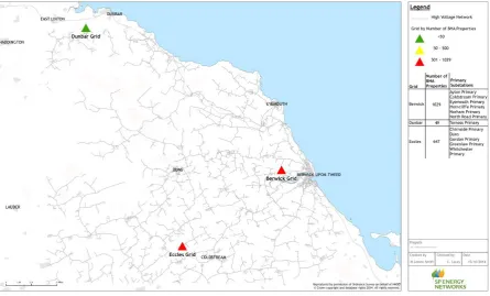
[image:11.595.118.480.314.536.2]The area proposed for BHA PV installations falls within an area of the electrical distribution network that is focus of the ARC project. In Figure 1, the ARC trial area is highlighted in green, and the area proposed for BHA PV installations is within the black circle.
Figure 1: The ARC trial area and an area proposed for BHA PV installations
An initial assessment of locations was carried out, and all proposed properties were plotted geographically onto maps of the distribution network, to identify the areas that may be subject to high penetration of PV installations. Figure 2 shows a number of BHA properties aggregated to Grid Supply Points (GSPs). It can be seen that most properties, 1029, are supplied from Berwick GSP from 6 primary substations, followed by Eccles GSP with 647 properties and 49 properties at Dunbar GSP connected to Torness primary substation.
Figure 2: Number of PV approved properties aggregated to Grid Supply Points
The BHA properties were categorised at the primary substation level, distinguishing proposed PV approved properties and PV approved and worst performing properties, i.e. all-electric homes with less efficient heating systems. This analysis is presented in Figure 3. Most of the proposed properties were connected to Duns and Eyemouth primary substations, 136 and 272, respectively. Ayton and Chirnside primary substations had a number of proposed properties between 66 and 130. All other primary substations had less than 65 PV proposed properties and they are shown in green.
Figure 3: Number of PV approved properties aggregated to primary substations
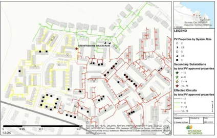
[image:12.595.77.520.443.717.2]Substation (S/S) site was carried out in order to identify the number of existing domestic PV systems, as some of the single installations were not recorded in SPEN’s GIS database. It was discovered, in this area, that only 30% of installed PV systems had been reported to SPEN and recorded on internal systems.
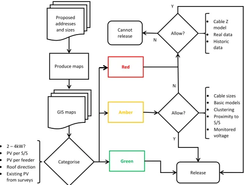
Each circuit ‘cluster’ was then further analysed to determine if potential PV generation would exceed voltage or thermal limits. Based on proposed PV system sizes, number of PVs per S/S, number of PVs per particular feeder and roof direction, all PV approved properties were categorised into three groups: green, amber, and red. Overall, 182 properties were categorised as green, 253 as amber, and 314 into as red. Figure 4 shows an example of PV approved properties clustered at a single S/S by system size. It can be seen that this particular S/S has three 3-phase LV feeders (green, amber and red) based on a number of proposed PV approved properties.
Figure 4: Example of PV approved properties at a single secondary substation
[image:13.595.87.512.217.487.2]All PVs within the green group of properties were approved for installation immediately by SPEN, as it was deemed that they would not have any significant negative impact on the network. At this stage, an agreed common document containing information and updates on progress was agreed between all parties to ensure one common point of truth. BHA and Edison Energy started their installation in February 2015. An example of installed BHA PV panels is shown in Figure 5.
proximity to S/S and monitored voltage at a secondary substation. After this additional analysis, these properties were either categorised as green and released or categorised as red for further analysis.
The red category LV circuits and hence substations were deemed most likely to have the greatest impact on the network and as such required a more detailed analysis. In addition to the installation of monitoring equipment at the secondary substations that supplied these properties, this analysis also included detailed modelling of each of the red category S/S, including their LV feeders and 11kV circuit they are connected to; and the load flow analysis based on real and historic data.
[image:14.595.59.547.208.577.2]The flowchart of the overall analysis explained above is presented in Figure 6.
Figure 6: The flowchart of the analysis3
3 A. Park, “Delivering Community Energy” Presented at Low Carbon Networks & Innovation (LCNI) Conference, Liverpool, Nov 2015.
Proposed addresses and sizes
Produce maps
GIS maps
2 – 4kW? PV per S/S PV per feeder Roof direction Existing PV
from surveys
Green Amber
Red
Release Categorise
Allow?
Cable sizes Basic models Clustering Proximity to
S/S Monitored
voltage voltage Allow?
Y N
Cable Z model Real data Historic
data Cannot
release
N
3
Monitoring and modelling
As detailed in section 2, PV approved properties in the amber and red categories had potential to have a significant influence on the network. The greatest impact would be seen on the secondary substation feeders where these PV panels would be connected. This could be due to the number and size of PV connections, the locations of panels, i.e. distance from the S/S or the network design. Therefore, these substations required additional, more detailed analysis that included the installation of monitoring equipment, detailed modelling of their respective 11kV circuits and LV feeders, and associated analysis based on real and historic data.
3.1
Monitoring equipment
As the traditional distribution LV network is passive, with limited monitoring data and no real-time controllability at secondary transformers, several secondary substations with properties within red and amber groups were fitted with advanced LV monitors. Overall, 22 monitors were installed at the locations shown in Figure 7, with four, more detailed regions shown in Figure 8. It is obvious that some of the susbstations are geographically next to each other and hence connected to the same 11kV circuit, especialy in the area 4. This cumulation can cause problems in the network, as the aggreagted generation can cause the distribution network to operate outside of its design limits.
Figure 8: Monitored secondary substations
The project selected two monitoring solutions, GMC-I METSyS4 and Gridkey MCU 5205. Both monitors are
powered via single phase voltage connection and they are totally protected against water and dust ingress (IP65). These monitors can monitor 3-phase voltage and current and up to maximum of 5 LV feeders in case of Gridkey MCU 520 and 6 LV feeders in case of GMC-I METSyS. Voltage connections for both monitors include: fused leads, busbar clamps, crimped lugs, dummy fuse and modified fuse holder. Current connections include Gridhound CTs and Rogowski coils for Gridkey MCU 520 monitor and Rogowski coils for GMC-I METSyS. Both monitors provide GPRS connection to SPEN’s iHost server. Figure 9 and Figure 10 show GMC-I METSyS and Gridkey MCU 520, respectively.
Figure 9: GMC-I METSyS substation monitor
4 GMC-I METSyS specifications: http://www.i-prosys.com/images/documents/GMC-I%20PORSyS%20(Compressed).pdf
Figure 10: Gridkey MCU 520 susbstation monitor
3.2
Modelling
Overall, fifteen secondary substations with their respective 11kV circuits and LV feeders were modelled in DIgSILENT PowerFactory software. These are highlited with red circles in Figure 7 and Figure 8, and they are: Ayton Lawfield, Briery Baulk, Buss Craig, Castle Street, Churchill, Deanhead, Dovecote, Dulcecraig, Grantshouse, Gunsgreenhill, Hawthorn Bank duns, Hoprig Road, Leitholm Village, Swinton Duns, and Chirnside West End. These substations differ in network topology, transformer ratings, numbers of customers connected and number of PV systems. They include mostly properties within red and amber groups, and they were likely to produce the greatest learning of the impact of solar panels on the distribution network.
Every modelled S/S has 11/0.4k33V 2-winding transformer, with reactance-to-resistance (X/R) ratio of 4.5% and a centre tap position of 0%. Transformer ratings and numbers of LV feeders of each modelled S/S are provided in Table 1.
Substation Name Transformer rating (MVA)
Number of LV feeders
Number of LV customers
Number of PV systems
Ayton Lawfield 0.5 3 73 24
Briery Baulk 0.3 3 129 17
Buss Craig 0.5 4 125 35
Castle Street 0.5 4 156 21
Churchill 0.5 4 91 20
Deanhead 0.5 4 242 39
Dovecote 0.3 3 127 51
Dulcecraig 0.5 3 180 42
Grantshouse 0.5 2 39 12
Gunsgreenhill 0.3 4 122 46
Hawthorn Bank Duns 0.5 3 111 15
Hoprig Road 0.5 4 99 38
Leitholm Village 0.3 3 94 19
Swinton Duns 0.2 2 54 20
West End Chirnside 0.8 6 162 52
PowerFactory, all fifteen models were developed manually which made this aspect of the project significantly more labour intensive than was anticipated.
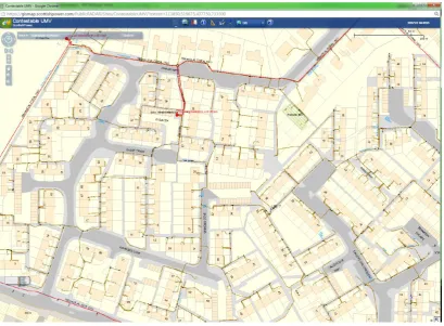
Figure 11: Example of SPEN's GIS system displaying a single substation with LV feeder cables and services
The network topology, cables and overhead lines (OHL), together with the type of conductor and its length are sourced directly from SPEN’s GIS database. SPEN’s LV network consists of a very large number of diverse aluminum and copper cables/OHL whose installation dates vary from 1930s until the present. Besides a large number of different cables/OHL types, there were also some errors in the GIS entries, e.g. in some cases 2 cores were recorded instead of 4 cores or types were unknown or missing. In such cases, and in the cases of very old cables/OHL, impedance and current ratings were not available in the present cable database, so they were assumed to be the same as the surrounding cables. A list with full specifications of all cables/OHL used and assumed in the modelling process is provided in Appendix 1.
Another challenge was to allocate a phase to each customer (load) and PV system, as SPEN’s GIS had no information available in some cases. Therefore, it was necessary to develop a systematic strategy to make assumptions, which included the following:
If the phase of a customer was known and phase of PV system was unknown, it was assumed that the PV system was (or would be) connected to the same phase as the customer.
If the phase of a customer was unknown, the customers together with PV systems were allocated a balanced rotation: red, yellow, blue.
Total numbers of PV systems and customers per each model are shown in Table 1, and their full lists, together with their phase allocation, are given in Appendix 3 and Appendix 4.
bus. Figure 13 presents the same area of SPEN’s network shown in Figure 11 migrated from GIS to PowerFactory. Detailed explanation of each model is provided in Appendix 2.
Figure 12: PowerFactory example of a single secondary substation with its respective 11kV circuits
4
Methodology, analysis and results
In order to analyse the impact of high penetration of PV systems installed on properties within the amber and red groups, LV monitoring equipment was installed on associated secondary substations and the University of Strathclyde developed different methodologies to investigate the potential headroom for new PV systems at each secondary substation. These methodologies have been used to develop PowerFactory scripts written in DIgSILENT Programming Language (DPL).
As previously discussed, SPEN has a requirement to ensure that the distribution network operates inside its design limits. The statutory voltage limits are as follows:
For the 11kV network: 11kV + / - 6% corresponding to 10.34kV – 11.66kV.
For the LV network: 230V +10% - 6% corresponding to 216.2V – 253V.
However, as limited monitoring equipment is connected at these voltage levels, and no real time control actions are possible, SPEN generally applies more stringent operational limits. When considering the connection of DG to an 11kV feeder, a typical operational voltage regime involves limiting the voltage at the point-of-connection of a generator to the maximum of 11.25kV under worst-case conditions (maximum DG output and minimum demand). The feeder is normally operated with the primary voltage set slightly higher than the nominal value as with low DG penetration, voltages will reduce along the feeder. The SPEN Design Manual6 suggests using 11.2kV as the primary voltage for DG studies if actual readings are not available. This
choice is made using through engineering experience and knowledge of the maximum expected voltage drops across the 11kV and LV networks.
In order to ascertain whether a number of PV installations could be connected to the network, clustering analysis was carried out as explained in Section 2. This analysis started in February 2015 and was reviewed a number of times throughout the year. During this time, fifteen secondary substation sites were modelled and analysed in PowerFactory, by running different load flow studies.
The aim of the PowerFactory analysis was to calculate a number of acceptable proposed PV systems under the worst-case conditions – highest solar irradiance and lowest network demand – whilst ensuring that network limits were maintained. In the case of PV systems, worst-case scenario normally occurs in summer time.
Different methodologies have been developed to analyse each secondary substation site under recorded and predicted conditions. These methodologies depended on the level of monitoring data available from each substation. The sites were only analysed during the daylight, as PV systems do not generate during the night. Every methodology assumed that PV panels should be prioritised based on electrical distance, with closest to the secondary substation first. The secondary LV voltages were simulated as the connected generation increased. The voltage was fixed at the primary substation. Recorded data included the following half-hourly data:
voltage at the primary substations,
LV voltage at modelled secondary substations, and
LV load data at modelled secondary substations – real and reactive power per each phase at each feeder.
After processing the data, three representative simulation time-steps were chosen, which correspond to the cases of minimum load at LV feeders and/or maximum LV voltages. Table 2 summarizes developed methodologies based on their input data.
Methodology Voltage at the primary recorded LV load data (P and Q) at modelled S/S
(i) Yes Recorded
(ii)-a No Recorded
(ii)-b No Predicted
Table 2: Summary of developed methodologies based on their input data
Methodology (i) was developed to investigate the potential headroom for new PV installations at a particular secondary substation under the recorded values of LV load and the voltage at the primary (recorded conditions). It includes the following steps:
1. Set the voltage at the primary to the recorded value.
2. Equally distribute recorded LV load (P and Q) along each of LV feeder at the particular S/S. 3. Set 11kV loads on other 11kV substations included in the model based on available data and
assumptions derived from these data.
4. Connect a PV (start from the electrically closest one to S/S). 5. Run an unbalanced load flow.
6. Check voltage and thermal limits at all locations and all phases. Satisfied?
7. If YES: Mark the last PV as acceptable, add the next electrically closest PV, and go to 5. 8. If NO: Go to 9.
9. Set the last PV out of operation, add the next electrically closest PV, and go to 5. 10. Stop when all PVs are checked.
Slightly modified methodology (ii) was developed to investigate a number of acceptable PV installations under the predicted conditions at a particular S/S, which include conditions when the voltage at the primary was not available. Therefore, this methodology calculates the voltage at the primary that allows connections of all proposed PV systems at the particular S/S. The starting point for the voltage at the primary is 11.2kV as suggested by SPEN Design Manual and decrease step size is 0.05kV. In addition, this methodology is further divided into two parts:
(ii)-a when LV load data at the particular S/S were available (recorded conditions) and
(ii)-b when LV load data at the particular S/S were not available (predicted conditions). It consists of the following steps:
1. Start from 11.2kV voltage at the primary. 2. Equally distribute:
2.1. recorded LV load along LV feeders – (ii)-a 2.2. predicted LV load along LV feeders – (ii)-b along each of LV feeder at the particular S/S.
3. Set 11kV loads on other 11kV substations included in the model based on available data and assumptions derived from these data.
4. Connect a PV (start from the electrically closest one to S/S). 5. Run an unbalanced load flow.
6. Check voltage and thermal limits at all locations and all phases. Satisfied?
7. If YES: Mark the last PV as acceptable, add the next electrically closest PV, and go to 5. 8. If NO: Go to 9.
9. Set the last PV out of operation, add the next electrically closest PV, and go to 5. 10.Check if all PVs are connected?
11.If NO: Decrease primary voltage for 0.05 and go to 2. 12.If YES: Stop.
analysed based on the methodology (i) apart from Hoprig Road and Chirnside West End, which were analysed based on the methodology (ii)-a as there were no available voltage data from the primary stations. The simulations were carried out for two different PV output scenarios:
PV panels export full installed capacity (100%) which is the worst-case scenario.
PV panels export 85% of their installed capacity.
The overall results suggested that the numbers of acceptable PV systems vary with their output capacity. There were no violations of thermal constraints and some of the PV installations were constrained by LV voltage limits at the connection terminals. These constrained PV systems were normally proposed to be connected at the end of an LV feeder. The results also suggested that the voltage at the secondary substation is dominated by the voltage at the primary, and in the cases of high primary voltage (above 11.1kV) less PV systems could be connected.
As the worst-case scenario (minimum demand and maximum PV generation) is expected to occur in summer time, in addition to the above analysis, it was important to investigate the values of the voltage at the primary that will allow the connection of all proposed PVs during summer time. Since in June 2015, summer data were still not available, second set of simulations for these six sites was carried out for predicted summer LV load data based on the methodology (ii)-b. These data were calculated based on the recorded winter data. The winter LV load was scaled to 50, 60, and 40% in order to investigate different scenarios for summer LV load. As expected, different levels of primary voltages that allow connections of all proposed PVs were found at different primary stations due to network topology, load level, number of PVs and their output. However, different voltage values were also found at Eyemouth primary for three sites connected to it. While the calculated primary voltage showed low values 10.45-10.7kV for Dulcecraig, it was around 10.95kV for Dovecote and Gunsgreenhill that are connected to same 11kV feeder.
Based on above simulations, SPEN was able to release more PV panels proposed to connect to these six S/S as well as to further re-cluster other red and amber sites. Following this process, nine additional S/S sites were fitted with LV monitors and modelled in PowerFactory. These are Ayton Lawfield and Grantshouse connected to Ayton primary; Briery Baulk, Castle Street, Hawthorn Bank Duns, and Leitholm Village connected to Duns primary; Churchill connected to Greenlaw; and Buss Craig and Deanhead connected to Eyemouth primary. Finally, third set of simulations for all fifteen modelled S/S was carried out in August 2015, when the recorded summer LV load data, June-July 2015, were available. These simulations were based on the methodologies (i) and (i)-a, for sites with no available primary voltage. They included three different PV output scenarios: 100, 90, and 85%. The third output scenario, 90%, was added based on SPEN’s Flexible Networks project7, which
finds 90% of PV output to be the most realistic measured maximum output capacity.
The overall results suggested that the numbers of acceptable PVs vary with their output capacity as it was expected. There were no thermal constraint violations and all not acceptable PVs were voltage constrained. For sites that were analysed for both predicted and recorded summer primary voltage and LV load data, when comparing the values of predicted voltage at the primary that allows connection of all proposed PVs and recorded primary voltage, it can be seen that for the values of recorded voltage higher than predicted ones, not all PVs could be connected.
The following subsections represent individual results for each of fifteen modelled secondary substations. First six S/S are the ones that were analysed for both recorded and predicted winter and summer data, and the others are additional S/S analysed only for recorded summer data.
4.1
Dovecote
Dovecote 3-phase LV network consists of three LV feeders and there are in total 127 loads and 51 proposed and existing PV systems. It is connected to Eyemouth primary at the same feeder as Buss Craig and Gunsgreenhill. Detailed explanation of the 11kV and LV models are provided in Appendix A 2.7.
An LV monitor at Dovecote S/S was installed in November 2014, so the analysis was carried out for both recorded and predicted data in winter and summer time.
At the time of the analysis for winter period, which was based on the methodology (i), there were 50 proposed PV systems. Table 3 shows a number of those PVs allowed to be installed per phase, for three different values of the voltage at the prymary measured at different dates and for two different PV output scenarios. The results suggest that all PVs could be connected at all times.
Recorded Winter load
PV 100% PV 85%
Primary V (kV), date 10.9, 18/3 10.964, 28/2 10.901, 10/3 10.9, 18/3 10.964, 28/2 10.901, 10/3
Phase A 19 19 19 19 19 19
Phase B 16 16 16 16 16 16
Phase C 15 15 15 15 15 15
Total 50 50 50 50 50 50
Table 3: Results at Dovecote S/S for winter period in 2015
Table 4 and Table 5 present a number of proposed PVs per each phase and the primary voltage that allows all proposed PV systems to be installed without violating network voltage limits for predicted summer loads and different PV output scenarios. These results are calculated following the methodology (ii)-b and they suggest that the voltage at the primary should be at 10.95kV in all casses.
Assumed Summer load, PV 100%
Winter load scaled to 0.5% Winter load scaled to 0.6% Winter load scaled to 0.4% Winter load date 18-Mar 28-Dec 10-Mar 18-Mar 28-Dec 10-Mar 18-Mar 28-Dec 10-Mar Phase A 19 19 19 19 19 19 19 19 19
Phase B 16 16 16 16 16 16 16 16 16
Phase C 15 15 15 15 15 15 15 15 15
Total 50 50 50 50 50 50 50 50 50 Primary V (kV) 10.95 10.95 10.95 10.95 10.95 10.95 10.95 10.95 10.95
Table 4: Results at Dovecote S/S for predicted summer loads in 2015 and 100% of PV output
Assumed Summer load, PV 85%
Winter load scaled to 0.5% Winter load scaled to 0.6% Winter load scaled to 0.4% Winter load date 18-Mar 28-Dec 10-Mar 18-Mar 28-Dec 10-Mar 18-Mar 28-Dec 10-Mar Phase A 19 19 19 19 19 19 19 19 19
Phase B 16 16 16 16 16 16 16 16 16
Phase C 15 15 15 15 15 15 15 15 15
Total 50 50 50 50 50 50 50 50 50 Primary V (kV) 10.95 10.95 10.95 10.95 10.95 10.95 10.95 10.95 10.95
Table 5: Results at Dovecote S/S for predicted summer loads in 2015 and 85% of PV output
PV 100% PV 90% PV 85% Primary V (kV),
date
10.838, 24/6
10.903, 1/6
10.675, 24/7
10.838, 24/6
10.903, 1/6
10.675, 24/7
10.838, 24/6
10.903, 1/6
10.675, 24/7
Phase A 16 16 16 16 16 16 16 16 16
Phase B 16 16 16 16 16 16 16 16 16
Phase C 15 15 15 15 15 15 15 15 15
Total 47 47 47 47 47 47 47 47 47
Table 6: Results at Dovecote S/S for summer period in 2015
4.2
Gunsgreenhill
Gunsgreenhill 3-phase LV network consists of four LV feeders and there are in total 122 loads and 46 proposed and existing PV systems. It is connected to Eyemouth primary at the same feeder as Dovecote and Buss Craig. Detailed explanation of the 11kV and LV models are provided in Appendix A 2.10.
An LV monitor at Gunsgreenhill S/S was installed in November 2014, so the analysis was carried out for both recorded and predicted data in winter and summer time.
At the time of the analysis for winter period, which was based on the methodology (i), there were 38 proposed PV systems. Table 7 shows a number of those PVs allowed to be installed per phase for three different values of the voltage at the prymary at different dates and for two different PV output scenarios. As in the case of Dovecote S/S, the results suggest that all PVs could be allowed at all times.
Recorded Winter load
PV 100% PV 85%
Primary V (kV), date 10.982, 1/1 11.034, 28/12 10.899, 10/3 10.982, 1/1 11.034, 28/12 10.899, 10/3
Phase A 14 15 15 15 15 15
Phase B 11 11 11 11 11 11
Phase C 11 12 12 12 12 12
Total 36 38 38 38 38 38
Table 7: Results at Gunsgreenhill S/S for winter period in 2015
Table 8 and Table 9 present a number of proposed PVs per each phase and the primary voltage that allows all proposed PV systems to be installed without violating network voltage limits for predicted summer loads and different PV output scenarios. These results are calculated following the methodology (ii)-b and they suggest that the voltage at the primary should be in a range of 10.9-11kV, depending on load level and PV output.
Assumed Summer load, PV 100%
Winter load scaled to 0.5% Winter load scaled to 0.6% Winter load scaled to 0.4% Winter load date 01-Jan 28-Dec 10-Mar 01-Jan 28-Dec 10-Mar 01-Jan 28-Dec 10-Mar
Phase A 15 15 15 15 15 15 15 15 15
Phase B 11 11 11 11 11 11 11 11 11
Phase C 12 12 12 12 12 12 12 12 12
Total 38 38 38 38 38 38 38 38 38 Primary V (kV) 10.9 10.95 10.9 10.9 10.95 10.9 10.85 10.9 10.9
Table 8: Results at Gunsgreenhill S/S for predicted summer loads in 2015 and 100% of PV output
Assumed Summer load, PV 85%
Winter load scaled to 0.5% Winter load scaled to 0.6% Winter load scaled to 0.4% Winter load date 01-Jan 28-Dec 10-Mar 01-Jan 28-Dec 10-Mar 01-Jan 28-Dec 10-Mar
Phase A 15 15 15 15 15 15 15 15 15
Phase B 11 11 11 11 11 11 11 11 11
Phase C 12 12 12 12 12 12 12 12 12
Total 38 38 38 38 38 38 38 38 38 Primary V (kV) 10.95 10.95 10.95 10.95 11 10.95 10.9 10.95 10.95
4.3
Dulcecraig
Dulcecraig 3-phase LV network consists of three LV feeders and there are in total 180 loads and 42 proposed and existing PV systems. It is connected to Eyemouth primary at the same feeder as Denahead. Detailed explanation of the 11kV and LV models are provided in Appendix A 2.8.
An LV monitor at Dulcecraig S/S was installed in November 2014, so it was analysed for both recorded and predicted data in winter and summer time.
At the time of the analysis for winter period, which was based on the methodology (i), there were 17 proposed PV systems. Table 10 shows a number of those PVs allowed to be installed per phase for three different values of the voltage at the prymary at different dates and for two different PV output scenarios. It can be seen that decreasing PV outputs to 85% on their installed capacity would allow the installations of all of them when the voltage at the primary is lower than 10.9kV.
Recorded Winter load
PV 100% PV 85%
Primary V (kV), date 10.838, 19/3 11.033, 8/3 11.033, 1/2 10.838, 19/3 11.033, 8/3 11.033, 1/2
Phase A 0 0 0 7 0 0
Phase B 0 0 0 5 0 0
Phase C 0 0 0 5 0 0
Total 0 0 0 17 0 0
Table 10: Results at Dulcecraig S/S for winter period in 2015
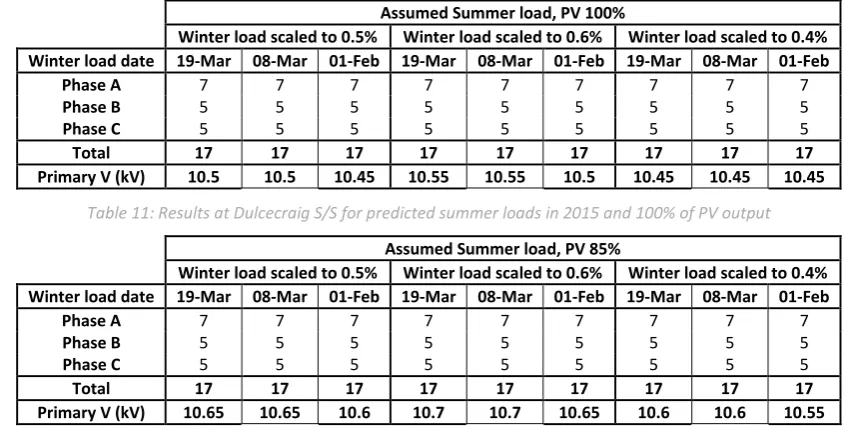
Table 11 and Table 12 present present a number of proposed PVs per each phase and the primary voltage that allows all proposed PV systems to be installed without violating network voltage limits for predicted summer loads and different PV output scenarios. These results are calculated following the methodology (ii)-b and they suggest that the voltage at the primary should be very low, in range of 10.5-10.65kV in order to allow all proposed PVs to connect.
Assumed Summer load, PV 100%
Winter load scaled to 0.5% Winter load scaled to 0.6% Winter load scaled to 0.4% Winter load date 19-Mar 08-Mar 01-Feb 19-Mar 08-Mar 01-Feb 19-Mar 08-Mar 01-Feb
Phase A 7 7 7 7 7 7 7 7 7
Phase B 5 5 5 5 5 5 5 5 5
Phase C 5 5 5 5 5 5 5 5 5
[image:25.595.83.509.427.640.2]Total 17 17 17 17 17 17 17 17 17 Primary V (kV) 10.5 10.5 10.45 10.55 10.55 10.5 10.45 10.45 10.45
Table 11: Results at Dulcecraig S/S for predicted summer loads in 2015 and 100% of PV output
Assumed Summer load, PV 85%
Winter load scaled to 0.5% Winter load scaled to 0.6% Winter load scaled to 0.4% Winter load date 19-Mar 08-Mar 01-Feb 19-Mar 08-Mar 01-Feb 19-Mar 08-Mar 01-Feb
Phase A 7 7 7 7 7 7 7 7 7
Phase B 5 5 5 5 5 5 5 5 5
Phase C 5 5 5 5 5 5 5 5 5
Total 17 17 17 17 17 17 17 17 17 Primary V (kV) 10.65 10.65 10.6 10.7 10.7 10.65 10.6 10.6 10.55
Table 12: Results at Dulcecraig S/S for predicted summer loads in 2015 and 85% of PV output
PV 100% PV 90% PV 85% Primary V (kV),
date
11.11, 8/7
11.12, 31/7
11.02, 16/7
11.11, 8/7
11.12, 31/7
11.02, 16/7
11.11, 8/7
11.12, 31/7
11.02, 16/7
Phase A 4 4 4 4 4 4 4 4 4
Phase B 4 5 5 4 5 5 5 5 5
Phase C 3 4 4 4 5 5 4 5 5
Total 11 13 13 12 14 14 13 14 14
Table 13: Results at Dulcecraig S/S for summer period in 2015
4.4
Hoprig Road
Hoprig Road 3-phase LV network consists of four LV feeders and there are in total 99 loads and 38 proposed and existing PV systems. It is connected to Torness primary and detailed explanation of the 11kV and LV models are provided in Appendix A 2.12.
An LV monitor at Hoprig Road S/S was installed in November 2014, so the analysis was carried out for both recorded and predicted data in winter and summer time.
At the time of the analysis for winter period there were 23 proposed PV systems. As there are no iHost data from Torness primary, the methodology (i)-a was applied, i.e. there was calculated the voltage at the primary that will allow connections of all proposed PV systems. The number of proposed PVs per each phase and the calculated primary voltage are shown in Table 14.
Recorded Winter load PV 100% PV 85%
Primary V (kV), date 24-Feb 10-Jan 10-Mar 24-Feb 10-Jan 10-Mar Phase A 6 6 6 6 6 6
Phase B 4 4 4 4 4 4
Phase C 13 13 13 13 13 13
Total 23 23 23 23 23 23 Primary V (kV) 11.05 11.2 11.1 11.15 11.2 11.2
Table 14: Results at Hoprig Road S/S for winter period in 2015
Table 15 and Table 16 present the values of the voltage at the primary that allows all proposed PV systems to be installed without violating network voltage limits for predicted summer loads and different PV output scenarios. These results are calculated following the methodology (ii)-b and they suggest that the voltage at the primary should be in a range of 10.75-11.05kV, depending on load level and PV output.
Assumed Summer load, PV 100%
Winter load scaled to 0.5% Winter load scaled to 0.6% Winter load scaled to 0.4% Winter load date 24-Feb 10-Jan 10-Mar 24-Feb 10-Jan 10-Mar 24-Feb 10-Jan 10-Mar
Phase A 6 6 6 6 6 6 6 6 6
Phase B 4 4 4 4 4 4 4 4 4
Phase C 13 13 13 13 13 13 13 13 13
Total 23 23 23 23 23 23 23 23 23 Primary V (kV) 10.8 10.9 10.8 10.85 10.95 10.9 10.75 10.8 10.75
Table 15: Results at Hoprig Road S/S for predicted summer loads in 2015 and 100% of PV output
Assumed Summer load, PV 85%
Winter load scaled to 0.5% Winter load scaled to 0.6% Winter load scaled to 0.4% Winter load date 24-Feb 10-Jan 10-Mar 24-Feb 10-Jan 10-Mar 24-Feb 10-Jan 10-Mar
Phase A 6 6 6 6 6 6 6 6 6
Phase B 4 4 4 4 4 4 4 4 4
Phase C 13 13 13 13 13 13 13 13 13
Total 23 23 23 23 23 23 23 23 23 Primary V (kV) 10.9 11 10.9 10.95 11.05 10.95 10.8 10.9 10.85
4.5
Swinton Duns
Swinton Duns 3-phase LV network consists of two LV feeders and there are in total 54 loads and 20 proposed and existing PV systems. It is connected to Norham primary and detailed explanation of the 11kV and LV models are provided in Appendix A 2.14.
An LV monitor at Swinton Duns S/S was installed in November 2014, so the analysis was carried out for both recorded and predicted data in winter and summer time.
At the time of the analysis for winter period, which was based on the methodology (i), there were 19 proposed PV systems. Table 17 shows a number of those PVs allowed to be installed per phase for three different values of the voltage at the prymary at different dates and for two different PV output scenarios. While a number of acceptable PVs is not affected by their generation output in the cases of lower primary voltage, it can be seen that this number varies when the voltage at the primary has higher value.
Recorded Winter load
PV 100% PV 85%
Primary V (kV), date 10.972, 19/3 11.164, 14/3 11.066, 2/3 10.972, 19/3 11.164, 14/3 11.066, 2/3
Phase A 5 4 5 5 5 5
Phase B 8 5 8 8 8 8
Phase C 6 5 6 6 6 6
Total 19 14 19 19 19 19
Table 17: Results at Swinton Duns S/S for winter period in 2015
Table 18 and Table 19 present a number of proposed PVs per each phase and the primary voltage that allows all proposed PV systems to be installed without violating network voltage limits for predicted summer loads and different PV output scenarios. These results are calculated following the methodology (ii)-b and they suggest that the voltage at the primary should be in a range of 11-11.1kV, depending on load level and PV output.
Assumed Summer load, PV 100%
Winter load scaled to 0.5% Winter load scaled to 0.6% Winter load scaled to 0.4% Winter load date 19-Mar 14-Mar 02-Mar 19-Mar 14-Mar 02-Mar 19-Mar 14-Mar 02-Mar
Phase A 5 5 5 5 5 5 5 5 5
Phase B 8 8 8 8 8 8 8 8 8
Phase C 6 6 6 6 6 6 6 6 6
[image:27.595.80.515.425.646.2]Total 19 19 19 19 19 19 19 19 19 Primary V (kV) 11 11.05 11 11.05 11.05 11 11 11 11
Table 18: Results at Swinton Duns S/S for predicted summer loads in 2015 and 100% of PV output
Assumed Summer load, PV 85%
Winter load scaled to 0.5% Winter load scaled to 0.6% Winter load scaled to 0.4% Winter load date 19-Mar 14-Mar 02-Mar 19-Mar 14-Mar 02-Mar 19-Mar 14-Mar 02-Mar
Phase A 5 5 5 5 5 5 5 5 5
Phase B 8 8 8 8 8 8 8 8 8
Phase C 6 6 6 6 6 6 6 6 6
Total 19 19 19 19 19 19 19 19 19 Primary V (kV) 11.05 11.05 11.05 11.05 11.1 11.05 11 11.05 11
Table 19: Results at Swinton Duns S/S for predicted summer loads in 2015 and 85% of PV output
PV 100% PV 90% PV 85% Primary V (kV),
date
11.11, 8/7
11.12, 31/7
11.02, 16/7
11.11, 8/7
11.12, 31/7
11.02, 16/7
11.11, 8/7
11.12, 31/7
11.02, 16/7
Phase A 4 4 4 4 4 4 4 4 4
Phase B 4 5 5 4 5 5 5 5 5
Phase C 3 4 4 4 5 5 4 5 5
Total 11 13 13 12 14 14 13 14 14
Table 20: Results at Swinton Duns S/S for summer period in 2015
4.6
Chirnside West End
Chirnside West End 3-phase LV network consists of six LV feeders and there are in total 164 loads and 52 proposed and existing PV systems. It is connected to Chirnside primary and detailed explanation of the 11kV and LV models are provided in Appendix A 2.15.
An LV monitor at Hoprig Road S/S was installed in November 2014, so the analysis was carried out for both recorded and predicted data in winter and summer time.
At the time of the analysis for winter period there were 31 proposed PV systems. As there are no iHost data from Chirnside primary, the methodology (i)-a was applied, i.e. there was calculated the voltage at the primary that will allow all proposed PV systems to be installed. The number of proposed PVs per each phase and the calculated primary voltage are shown in Table 21.
Recorded Winter load PV 100% PV 85%
Primary V (kV), date 19-Mar 26-Dec 04-Jan 19-Mar 26-Dec 04-Jan Phase A 12 12 12 12 12 12
Phase B 13 13 13 13 13 13
Phase C 6 6 6 6 6 6
Total 31 31 31 31 31 31 Primary V (kV) 10.95 11.05 10.95 11 11.05 11
Table 21: Results at Chirnside West End S/S for winter period in 2015
Table 22 and Table 23 present a number of proposed PVs per each phase and the primary voltage that allows all proposed PV systems to be installed without violating network voltage limits for predicted summer loads and different PV output scenarios. These results are calculated following the methodology (ii)-b and they suggest that the voltage at the primary should be in range of 10.9-11.05kV, depending on load level and PV output.
Assumed Summer load, PV 100%
Winter load scaled to 0.5% Winter load scaled to 0.6% Winter load scaled to 0.4% Winter load date 19-Mar 26-Dec 04-Jan 19-Mar 26-Dec 04-Jan 19-Mar 26-Dec 04-Jan Phase A 12 12 12 12 12 12 12 12 12
Phase B 13 13 13 13 13 13 13 13 13
Phase C 6 6 6 6 6 6 6 6 6
Total 31 31 31 31 31 31 31 31 31 Primary V (kV) 10.9 11.05 10.95 10.95 11.05 10.95 10.9 11 10.9
Table 22: Results at Chirnside West End S/S for predicted summer loads in 2015 and 100% of PV output
Assumed Summer load, PV 85%
Winter load scaled to 0.5% Winter load scaled to 0.6% Winter load scaled to 0.4% Winter load date 19-Mar 26-Dec 04-Jan 19-Mar 26-Dec 04-Jan 19-Mar 26-Dec 04-Jan Phase A 12 12 12 12 12 12 12 12 12
Phase B 13 13 13 13 13 13 13 13 13
Phase C 6 6 6 6 6 6 6 6 6
Total 31 31 31 31 31 31 31 31 31 Primary V (kV) 10.95 11.05 10.95 10.95 11.05 10.95 10.95 11.05 10.95
At the time of the analysis for summer period, 3 out of 31 PVs have already been installed and there were still 28 proposed PV installations. As there were no iHost data from Chirnside primary, the voltage at the primary that will allow all proposed PV systems to be installed was calculated based on the methodology (i)-a. The results are shown in Table 24.
Recorded Summer load
PV 100% PV 90% PV 90% Primary V, date 02-Jul 08-Jun 15-Jul 02-Jul 08-Jun 15-Jul 02-Jul 08-Jun 15-Jul
Phase A 10 10 10 10 10 10 10 10 10
Phase B 12 12 12 12 12 12 12 12 12
Phase C 6 6 6 6 6 6 6 6 6
Total 28 28 28 28 28 28 28 28 28 Primary V (kV) 10.95 10.95 10.95 10.95 10.95 10.95 11 11 10.95
Table 24: Results at Chirnside West End S/S for summer period in 2015
4.7
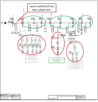
Ayton Lawfield
Ayton Lawfield 3-phase LV network consists of three LV feeders, and there are in total 73 loads and 24 proposed and existing PV systems. It is connected to Ayton primary and detailed explanation of the 11kV and LV models are provided in Appendix A 2.1.
An LV monitor at Ayton Lawfield S/S was installed in May 2015, so only the analysis for recorded summer data based the methodology (i) was carried out. There were six proposed PV installations, and Table 25 shows a number of those PVs allowed to be installed per phase for three different values of the voltage at the prymary at different dates and for three different PV output scenarios.
Recorded Summer load
PV 100% PV 90% PV 85%
Primary V (kV), date
11.06, 21/7
11.237, 3/7
11.134, 25/7
11.06, 21/7
11.237, 3/7
11.134, 25/7
11.06, 21/7
11.237, 3/7
11.134, 25/7
Phase A 0 0 0 0 0 0 0 0 0
Phase B 0 0 0 0 0 0 0 0 0
Phase C 0 0 0 0 0 0 0 0 0
Total 0 0 0 0 0 0 0 0 0
Table 25: Results at Ayton Lawfield S/S for summer period in 2015
It can be seen that none of the proposed PV installations were allowed to connect under these network conditions. Ayton Lawfield S/S is the first S/S next to the primary and hence its voltage is highly influenced by the primary voltage, which is above 11kV most of the time. All of these PVs are voltage constrained, as they would cause a rise of the voltage at Ayton Lawfield S/S above network limits, 253V.
4.8
Briery Baulk
Briery Baulk 3-phase LV network consists of three LV feeders and there are in total 129 loads and 17 proposed and existing PV systems. It is connected to Duns primary and detailed explanation of the 11kV and LV models are provided in Appendix A 2.2.
PV 100% PV 90% PV 85% Primary V (kV),
date 11.021, 31/7 11.119, 22/6 10.968, 19/7 11.021, 31/7 11.119, 22/6 10.968, 19/7 11.021, 31/7 11.119, 22/6 10.968, 19/7 Constraints Not
satisfied
Not
satisfied Satisfied
Not satisfied
Not
satisfied Satisfied Satisfied
Not
satisfied Satisfied
Table 26: Results at Briery Baulk S/S for summer period in 2015
4.9
Buss Craig
Buss Craig 3-phase LV network consists of four LV feeders and there are in total 125 loads and 35 proposed and existing PV systems. It is connected to Eyemouth primary at the same feeder as Dovecote and Gunsgreenhill. Detailed explanation of the 11kV and LV models are provided in Appendix A 2.3
An LV monitor at Buss Craig S/S was installed in March 2015, so only the analysis for summer period based on the methodology (i) was carried out. There were 13 proposed PV installations. Table 27 shows a number of those PVs allowed to be installed per phase for three different values of the voltage at the prymary at different dates and for three different PV output scenarios.
Recorded Summer load
PV 100% PV 90% PV 85%
Primary V (kV), date 10.622, 9/7 10.884, 4/6 10.666, 24/7 10.622, 9/7 10.884, 4/6 10.666, 24/7 10.622, 9/7 10.884, 4/6 10.666, 24/7
Phase A 5 0 5 5 1 5 5 1 5
Phase B 5 0 5 5 1 5 5 2 5
Phase C 3 1 3 3 1 3 3 2 3
Total 13 1 13 13 3 13 13 5 13
Table 27: Results at Buss Craig S/S for summer period in 2015
It can be seen that the voltage at the primary is in range of 10.6-10.9kV and PV installations are constrained only in the case of its higher values.
4.10
Castle Street
Castle Street 3-phase LV network consists of four LV feeders and there are in total 156 loads and 21 proposed and existing PV systems. It is connected to Duns primary and detailed explanation of the 11kV and LV models are provided in Appendix A 2.4.
An LV monitor at Castle Street S/S was installed in May 2015, so only the analysis for summer period based on the methodology (i) was carried out. There were eight proposed PV installations. Table 28 shows a number of those PVs allowed to be installed per phase for three different values of the voltage at the prymary at different dates and for three different PV output scenarios. As expected, the results suggest that in the cases of higher voltage at the primary not all PVs could be connected.
Recorded Summer load
PV 100% PV 90% PV 85%
Primary V (kV), date 11.045, 19/7 11.119, 22/6 11.039, 26/7 11.045, 19/7 11.119, 22/6 11.039, 26/7 11.045, 19/7 11.119, 22/6 11.039, 26/7
Phase A 2 0 2 2 0 2 1 1 2
Phase B 3 0 3 3 0 4 4 1 4
Phase C 2 0 2 2 1 2 2 1 2
Total 7 0 7 7 1 8 7 3 8
Table 28: Results at Castle Street S/S for summer period in 2015