Nonlinear predictive generalized minimum variance LPV control of wind turbines

Nonlinear Predictive Generalized Minimum Variance LPV

Control of Wind Turbines

P Savvidis*, M J Grimble

*Industrial Control Centre (ICC), University of Strathclyde, Glasgow, UK, [email protected] , † Industrial Control Centre (ICC), University of Strathclyde, Glasgow, UK, [email protected], ††Industrial Systems & Control Limited (ISC

Ltd), Glasgow, UK, [email protected], †††Dalian University of Technology, China, [email protected]

Keywords: Wind turbine, control, modelling, LPV,

predictive control.

Abstract

More advanced control strategies are needed for use with wind turbines, due to increases in size and performance requirements. This applies to both individual wind turbine controls and for the total coordinated controls for wind farms. The most successful advanced control method used in other industries is predictive control, which has the unique ability to handle hard constraints that limit system performance. However, wind turbine control systems are particularly difficult in being very nonlinear and dependent upon the external parameter variations which determine behaviour. Nonlinear controllers are often complicated to implement. The approach proposed here is to use one of the latest predictive control methods which can be used with linear parameter varying (LPV) models. These can approximate the behaviour of nonlinear wind turbines and provide a simpler control structure to implement. The work has demonstrated the feasibility and benefits that may be obtained.

1 Introduction

There has been a lot of interest in the application of advanced controls to wind turbine systems. The use of LPV models has been discussed previously [1, 2]. However, new controllers have been developed for industrial processes particularly aimed at generating relatively simple designs to understand and implement. Work in the Industrial Control Centre at the University of Strathclyde on Nonlinear Generalised Minimum Variance controllers (supported by the EPSRC) has led to a family of controllers, including predictive versions that have shown great potential. The company established by the University almost 30 years ago (Industrial Systems and Control Ltd.) to encourage technology transfer into industry, has used these design approaches extensively across industrial sectors. The benefits of the algorithms have been demonstrated in a PhD thesis by Savvidis (2016). This has assessed the design methods in a range of applications and one of the most promising was the wind energy problem considered here. In fact, joint work with Professor Yang Pang has revealed the design approached apply to a very wide class of industrial processes including hybrid systems.

The particular features of the design methods which are valuable for the wind turbine control problem include the flexible way to model the process and the very general criterion that may be optimised. This criterion can have nonlinear terms and if for example fatigue is being minimised in wind turbines this is a useful asset. There are not many control techniques which enable a nonlinear cost-function to be minimised using a rigorous theoretical solution and at the same time an algorithm which is relatively simple to understand and implement. The main feature of the following work is the demonstration of how the controllers are used and the benefits that are available.

2 Problem Description

The main objective of the control solution proposed in this paper is the regulation of produced electrical power in a large scale wind turbines. This is achieved at the turbine rated power [3, 4], while compensating for:

• Nonlinearities in the mechanical parts of the turbine (e.g. actuator range limits) and in the aerodynamic conversion between wind energy and electrical power. • Wind disturbances (i.e. sudden wind gusts and

turbulent wind variations).

Using the same control paradigm, a secondary scenario is explored, that of varying the power output demand of the turbine (derating). This is particularly useful in centralised wind farm power production control. In the latter case, individual turbines are required to reduce their output so that an optimal total output is reached with respect to various criteria like the minimisation of mechanical loading in the turbine, maximisation of power produced etc. [5].

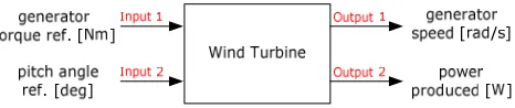
The wind turbine control strategy described in this section incorporates two separate configurations, a Single-Input-Single-Output (SISO) and a Multiple-Input-Multiple-Output (MIMO) control system as explained in Section 4 [3, 6]. Figure 1 illustrates the Control Variables (CV) and Plant Variables (PV) utilised for control.

1. Fixed-Torque/Variable-Pitch; the generator torque is

2. Variable-Torque/Variable-Pitch; both the generator torque and pitch are manipulated to regulate the generator speed and power respectively at the rated value, during wind speed variations.

Figure 1: MIMO System MV/CV variables (the SISO case is

the subset Input 2/Output 2).

When the wind turbine operates in the below rated wind speed region control strategies mostly aim at the maximisation of produced electrical power. Throughout this mode of operation the blade pitch is set to zero to allow as much as possible of the energy available in the wind to be harvested. At the same time the torque reference to the generator is derived from optimal lookup tables implemented within the controller [7]. For this application however the focus goes to the above rated operating region where the main control objective becomes the regulation of the produced electrical power at its rated value, also limited by the generator speed rating.

3 Wind Turbine System Description

The wind turbine system used within this work is a theoretical model, representative of a utility-scale multi-megawatt Wind Energy Conversion System (WECS) developed by the National Renewable Energy Laboratory (NREL) and thoroughly validated against real systems [7]. More specifically, it is a three-bladed upwind, 5MW wind turbine with active pitch control and Doubly-Fed Induction Generator (DFIG) with controllable generator torque. The overall wind turbine from a systems standpoint is a combination of static and dynamic, linear and nonlinear components. The following list contains those sub-systems that are vital for control design,

1. Pitch Actuator; linear-dynamic, 2. Rotor Aerodynamics; nonlinear-static, 3. Transmission; linear-dynamic,

4. Generator & Converter; linear-dynamic.

The principal objective of a WECS is to convert kinetic energy out of the wind into electrical power. The first conversion occurs in the rotor of the turbine where wind power is translated into mechanical power and subsequently translated into electrical through the transmission and generator components. The amount of power which could be extracted by the wind is determined by the area swept by the turbine rotor and is limited by a factor which varies with the tip speed ratio and the pitch angle of the blade [6].

The overall wind turbine subsystems equations for the purpose of control are described in detail in [3]. For a detailed description of the 5MW NREL subsystems interconnections see [7]. Also note the wind speed feeding into the rotor aerodynamics calculation is actually the effective wind speed defined as the difference between the actual and the turbine tower velocity .

3.1 LPV Model for Wind Turbine Control

This section presents the total integrated and discretised linear parameter varying (LPV) model used within the Nonlinear Predictive Generalized Minimum Variance (NPGMV) controller. The model reflects small deviations along the optimal trajectory. Is consists of all the sub-systems that were described in the previous section and summarised below. All subsystems are essentially linear except from the aerodynamic conversion equations for the power, rotor torque and thrust force. These are parameterised by wind speed, pitch angle and tip speed ratio through the equivalent efficiency coefficients (Cp etc.) and therefore linearized

across the optimal trajectory for the purposes of control design.

The fully integrated LPV model used within the controller is shown in Equations 1, 2. For a detailed description of the derivation see [2].

State vector:

x1 : Blade pitch angle

= =

x2 : Blade pitch rate

x3 : Low speed shaft torsional angle x4 : Generator speed

x5 : Rotor speed

x6 : Generator load torque x7 : Tower fore-aft displacement x8 : Tower fore-aft velocity

Input vector:

u1 : Blade effective wind speed

= = _ _"

u2 : Generator load torque reference u3 : Pitch angle reference

Output vector:

y1 : Generator speed

# = ##

#" = $%

"

y2 : Blade pitch angle y3 : Produced electrical power

Complete LPV Wind Turbine Model:

=

0 1 0 0 0 0 0 0

− ) −2+ ) 0 0 0 0 0 0

0 0 0 −_,1 1 0 0 0

0 0 _,/-%. −_{, /}0%. −_,/0%. −_/1 0 0

1234

/ 0 −

-%.

/ −

0%.

/ −

(0%.+ 12₃₇₃)

,/ 0 0 −

12_39:;; /

0 0 0 0 0 −<= 0 0

0 0 0 0 0 0 0 1

1_>4

? 0 0 0 −

1_>73

? 0 −?- −

+

0 0 0

0 0 )

0 0 0

0 0 0

123_@:;;

/ 0 0

0 <= 0

0 0 0

1_>_@:;;

? 0 0

(1)

# = A

0 0 0 1 0 0 0 0

B

180 0 0 0 0 0 0 0

0 0 0 _DE 0 _DE 0 0

F (2)

To derive the LPV model of the wind turbine, the nonlinear terms (Cq and Ct coefficients lookup tables in this case) are first linearized, then interpolated and parameterised by wind speed to yield the corresponding deviations model along these optimal curves. In Equation 3 a modification to the standard Jacobian linearization is seen which is not restricted to equilibrium points (derivative terms are maintained).

G HIJ = K1( H, H) − MHIK N HI

− OHIK N HIN

+ MHIK N I+ OHIK N I

G#HI = KP( H, H) − QHIK N HIN

+ QHIK N I

(3)

4 Control Architecture & Design

4.1 Control Architecture

The architecture used is composed of a feedback and a feedforward component, where feedforward action establishes the nominal operating point at every step and feedback action compensated for deviations around that operating point. This is summarised in Figure 2 for the SISO case.

Feedback Action; this component is used to minimise power

variations around the rated value and compensate for model uncertainties and nonlinearities.

Feedforward Action; this component is based on the optimal

trajectories for the pitch angle, rotor/generator speed, power and generator torque. Its main purpose is to provide control action that will keep power production at the rated value above rated wind speed - in the steady-state sense and assuming no modelling errors. The optimal reference curves, provided by the lookup tables, are also used to generate power and speed reference signals for the feedback controller. Note that for the above rated operation that is examined here only the pitch angle optimal curve varies whereas the power, generator speed and torque curves remain fixed at the corresponding rated values. The optimal curves for this particular wind turbine can be found in [7].

Figure 2: SISO Control System FB+FF structure.

4.2 LPV-NPGMV Controller Sub-systems Formulation

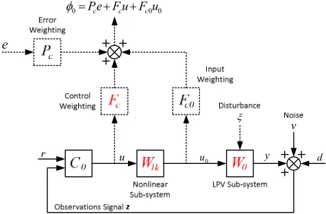
The basic Nonlinear Generalized Minimum Variance (NGMV) control structure is used as a common ground for this work and reviewed in Figure 3 [8]. The plant model, as seen here, is the decomposition of the full nonlinear plant into a general nonlinear operator W1k and an LPV approximation

W0. The nonlinear operator can be considered to include

unmodelled nonlinearities, represented as input nonlinearities. The LPV sub-system is used to accommodate LPV approximations of parts of the plant where possible and also disturbance and reference models.

e

r _u

0

u y d

v

ξ

0 0 0=Pce+Fcu+Fcu

φ

Figure 3: NPGMV Feedback Control Structure

Input Signals: r: reference, d: disturbance, ν: measurement noise.

Control Signals: u: control signal to NL subsystem, u0:

control inputs to LPV subsystem.

Output Signals: y: plant output signals, z: output

measurement signals

Error Signal: e: tracking error signals.

input and the measurements of the plant outputs to be controlled e(t)= r(t) – r(t).

Nonlinear Input Sub-System:

This sub-system is described by the following notation,

(R )(S) = TUI_{(RI )(S) (4)}

where z-k is a diagonal matrix that contains all common delay elements in signal paths, assuming these can be extracted out of the system. The output of R_I is denoted as, _H(S) =

(RI )(S), where, R_I is assumed to be finite gain stable. Note that k signifies the explicit delay elements that have been extracted from the full nonlinear plant system.

Nonlinear Output Sub-System:

This sub-system is also nonlinear of an LPV form and is denoted as,

(RH H)(S) = (RHITUI H)(S) (5)

where R_HI is its delay-free notation.

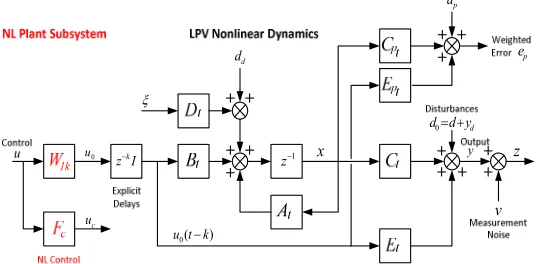
Nonlinear Output Sub-System (LPV Expansion):

The LPV output sub-system has the general structure shown in Figure 4, where M_V= M_HWXKS, _H(S − Y)NZ and ρ varies with time. The subscript t indicates that the matrices will now vary with time being dependant on ρ.

u u0

I z−k

c

u

ξ

1 −

z

) (

0t k

u −

d

d

p

d

v

y z

d

y d d0= +

x

p e

Figure 4: Generalised LPV Subsystems expansion

The weighted error ep equation is,

[E(S) = \E(S) + QEV (S) + ]EV H(S − Y) (6)

In Figure 7 disturbances are broken down into their stochastic and deterministic components. Each of the reference, disturbance and error weighting subsystems illustrated in the figure can be modelled individually in a state-space manner to compliment the LPV nonlinear dynamics. The derivation in which importance is given here is the augmented model which is used internally in the controller for nonlinear compensation.

Augmented System Derivation:

The overall sub-system in state-space form will be a multivariable _ × ? system that consists of the plant LPV dynamics, the disturbance and weighted error state-space models, integrated into a complete augmented representation [9]. This model will be a function of control and the varying parameters (considered in the LPV formulation (u0(t-k), ρ(t)).

The new state vector will be x=[x0, xd, xp].

For simplicity from this point onwards the LPV sub-system matrices will be denoted as A0, B0, C0 etc. The augmented

system state equations can be defined as follows.

= a M0H M0b 00

−OEQH −OEQH ME

c + O0H −OE]H

" HI

+ 00 0H 0b

0 0" d+ e + f 0 0 0 0 OE

" g \Hb

(_ − \)h

(7)

Similarly the error equation can be defined as follows.

[E= \b+ i−]EQH −]EQb QEj − ]E]H HI (8)

4.3 Predictions Model for Control

For the derivation of the NPGMV controller a model is required based on which predictions of the future outputs and output errors will be generated. This iterative derivation was described in detail in [10]. Here only the generalised predictions equations are included as reference, to provide coherence in flow for the derivation of the control law. The i-steps prediction for the state and the output signals can be summarised in the following manner.

k(S + l|S) =

MVnk(S|S) + ∑ Mnpr VJpnUpWOVJpU H(S + q − 1 −

Y) + \b(S + q − 1)Z (9)

#k(S + l|S) = \(S + l) + Q(S + l)k(S + l|S)

+ ](S + l) H(S + l − Y) (10)

Similarly the estimated weighted error equation is as follows. This is the signal to be regulated at future times (l ≥ 1).

[̂E(S + l|S) = \E(S + l) + QEVJn(S + l)k(S + l|S)

+ ]EVJn(S + l) H(S + l − Y) (11)

4.4 The LPV-NPGMV Optimal Control Solution

The cost function that needs to be minimised within this framework is shown below.

The future predicted values of uv_VJI,wH involve the estimated vector of weighted errors ]y_EVJIz,w which are orthogonal to

]{EVJIz,w. Moreover the estimation error is zero-mean and the expected value of the product with any known signal is null. The optimal control is the one that sets uv_VJI,wH to zero or as shown in the following equation.

|V,w= −K}=I,w+ ~wRI,wNU $=w]yEVJIz,w (13)

Note that in this paper only a brief mention of the full control law derivation is included.

5 Simulation Results

In this section the LPV-NPGMV is employed in the wind turbine system and performance is tested against two baseline controllers, a simple PID and the basic state-space NGMV. For this purpose various scenarios within the above rated operating region were used, only few representative presented in this paper. These include different types of wind speed variations (disturbance rejection) such as step changes, gusts and turbulence but also power reference variations (tracking). In the later the knowledge of future input signals option within the NPGMV controller is used. Two basic metrics are used to quantify these results and assist with assessing performance for each controller. These are the normalised STD of the MVs and the MISE for the CVs as shown below.

Scenario 1 – Small gust variation of 14-16m/s (nominal wind speed at 15m/s):

For this scenario the power reference to the turbine is kept constant at nominal value (5MW) whereas wind speed variation (around a nominal value of 15m/s) in the form of a gust is used as a disturbance to examine control compensation by the three controllers. Figure 5 captures the results for the SISO case followed by the quantified comparison results table for different prediction horizons Np.

Figure 5: Results for the SISO control structure

Generator speed, electric power and pitch angle are shown from upper to lower graphs respectively.

Controllers βSTD (norm.) PelMISE (norm.)

PID 1 1

NGMV 0.9862 0.3780

LPV-NPGMV [Np=3] 0.9911 0.2065

LPV-NPGMV [Np=5] 0.9927 0.1696

Table 1: Scenario 1, SISO quantified controller comparison.

Scenario 2 – Turbulent wind variation between 12-21m/s:

For this scenario the power reference to the turbine is kept constant at nominal value (5MW) whereas wind speed variation (around a nominal value of 15m/s) is disturbed by a stochastic turbulent component to examine control compensation by the three controllers. Only the quantified results table is included in this paper.

Controllers βSTD (norm.) PelMISE (norm.)

PID 0.6005 1

NGMV 0.7799 0.6642

LPV-NPGMV [Np=10] 0.8170 0.6291

LPV-NPGMV [Np=50] 1 0.3772

Table 2: Scenario 2, SISO quantified controller comparison.

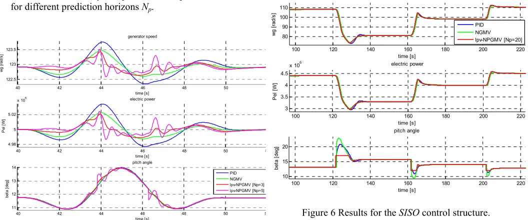
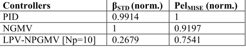
Scenario 3 – Sequence of steps in power between 0-2MW:

For this scenario wind speed is kept constant at above rated in order to provide rated power availability (5MW). A series of steps in power reference (between 0-2MW) are then introduced. Figure 6 captures the results on reference tracking for the SISO control structure. To explore performance of the LPV-NPGMV in the presence of constraints the pitch angle actuator range was limited between 12-17deg.

Figure 6 Results for the SISO control structure.

40 42 44 46 48 50 52

122.5 123 123.5

generator speed

time [s]

w

g

[

ra

d

/s

]

40 42 44 46 48 50 52

4.98 5 5.02

x 106 electric power

time [s]

P

e

l

[W

]

40 42 44 46 48 50 52

11 12 13 14

pitch angle

time [s]

b

e

ta

[

d

e

g

]

PID NGMV lpv-NPGMV [Np=3] lpv-NPGMV [Np=5]

100 120 140 160 180 200 220

80 90 100 110

generator speed

time [s]

w

g

[

ra

d

/s

]

100 120 140 160 180 200 220

3 3.5 4 4.5

x 106 electric power

time [s]

P

e

l

[W

]

100 120 140 160 180 200 220

10 15 20

pitch angle

time [s]

b

e

ta

[

d

e

g

]

Controllers βSTD (norm.) PelMISE (norm.)

PID 0.9914 1

NGMV 1 0.9197

LPV-NPGMV [Np=10] 0.2679 0.7541

Table 3: Scenario 3, SISO quantified controller comparison.

6 Conclusions

To be able to judge whether advanced controls provides an improvement some criteria should be established. However, there are many requirements of good wind turbine controllers and to some extent the decision is subjective. Nevertheless, the following advantages seem clear:

1. Most industries are moving towards using physical models on which to base control designs since this enables more formalised design procedures to be used and the predictive control methods lend themselves to such an approach.

2. To be able to benchmark the performance of the system a cost-function is often required and this is available in the methods proposed because of the problem of formulation. This can enable performance to be quantified and good control to be judged. 3. Classical controls can provide very adequate and good

solutions but when systems are interacting and multivariable they are very much more difficult to control and again the predictive control methods lend themselves to this problem.

4. Classical control methods also do not account for disturbances in a very formal or optimal manner but the predictive control solutions can use the statistical information on disturbances. In the wind energy problem this is of course a central feature of designs. 5. Most classical design methods do not take account of

nonlinearities very formally and the same applies to parameter variations rising in systems. The type of solution presented can account naturally for these difficulties.

There are of course obvious disadvantages of more advanced methods such as the additional complexity in both implementation and the levels of staff needed in the design office. However, with the increase in computing power over recent years and new formalised design procedures such problems are becoming less significant. It is of course the case that advanced controls will not be used if classical methods can be considered adequate, even if they provide some improvements. However, with the cost implications of faults and failures in large wind turbines, and with the loss in possible power output that may arise there is real imperative to use more advanced methods. It seems likely that in future years advanced controls will be considered a necessary evil and companies that do not adopt such philosophies will suffer the economic consequences.

Acknowledgements

The authors are grateful for the support from the University of Strathclyde in Glasgow and Industrial Systems & Control Ltd. in Glasgow, which was established by the University to encourage technology transfer.

References

[1] K. Z. Østergaard, P. Brath, J. Stoustrup. “Linear parameter varying control of wind turbines covering both partial load and full load conditions”, Int. J. of Robust and Nonlinear Control, volume. 19, pp. 92-116, (2009).

[2] F. D. Adegas, J. Stoustrup. “Structured Control of LPV Systems with Application to Wind Turbines”, American Control Conference, Fairmont Queen Elizabeth, Montréal, Canada, pp. 756-761, (2012).

[3] F. Bianchi, H. de Battista, R. Mantz. “Wind Turbine Control Systems: Principles, Modelling and Gain Scheduling Design”, Springer, (2007).

[4] D. J. Leith, W. E. Leithead. “Implementation of Wind Turbine Controllers”, International Journal of Control,

volume 66, Issue 3, pp. 349-380, (1997).

[5] AEOLUS FP7 Project: “Distributed Control of Large-scale Offshore Wind Farms”, http://www.ict-aeolus.eu/index.html.

[6] E.A Bossanyi. “The design of Closed Loop Controllers for Wind Turbines”, Wind Energy, Vol.3, pp.149-163., (2001).

[7] J. Jonkman, S. Butterfield, W. Musial, G. Scott. “Definition of a 5-MW Reference Wind Turbine for Offshore System Development”, Technical Report NREL/TP-500-38060, (2009).

[8] M. J. Grimble. “Non-linear generalised minimum variance feedback, feedforward and tracking control”, Automatica, volume 41, pp. 957-969, (2005).

[9] M. J. Grimble, Y. Pang. “NGMV Control of State Dependent Multivariable Systems”, Proceedings of the 46th IEEE Conf. on Decision and Control, New Orleans, LA, USA, pp. 1628-1633, (2007).