Using hydrodynamic models to understand the impacts and risks of plastic pollution

ResearchOnline@JCU

This file is part of the following work:

Critchell, Kay Lilian (2018)

Using hydrodynamic models to understand the

impacts and risks of plastic pollution.

PhD Thesis, James Cook University.

Access to this file is available from:

https://doi.org/10.25903/5bd25335639a2

Copyright © 2018 Kay Lilian Critchell

The author has certified to JCU that they have made a reasonable effort to gain

permission and acknowledge the owners of any third party copyright material

included in this document. If you believe that this is not the case, please email

Using hydrodynamic models to

understand the impacts and risks of

plastic pollution

PhD thesis submitted by: Kay Lilian Critchell

Bachelor of Marine Science (Hons), James Cook University

January 2018

For the degree of Doctor of Philosophy College of Science and Engineering

i the dominant physical processes? Estuarine, Coastal and Shelf Science. 2016; 171:111-22. Critchell K, Hoogenboom M. Effects of microplastic exposure on the body condition and behaviour of planktivorous reef fish (Acanthochromis polyacanthus) under review PlosONE

Critchell K, Hamann M, Grech A. A spatially explicit exposure analysis of plastic pollution in prep Critchell K, Hoogenboom M, Grech A, Hamann M, Wolanski E. Using field data to interrogate a plastics dispersal model in prep

Other publications

Critchell K, Bauer-Civiello A, Benham C, Berry K, Eagle L, Hamann M, Hussey K, Ridgway T, Plastic pollution in the coastal environment: Solutions into the future in Estuaries and Coasts: the Future eds. Wolanski E, Day J, Elliott M, and Ramachandran R in production

Hoogenboom M, Frank G, Alvarez M, Chase T, Critchell K, Berry K, Jurriaans S, Nicolet K, Peterson K, Ramsby B, Paley A. Environmental drivers of variation in bleaching severity of Acropora corals during an extreme thermal anomaly, Frontiers in Marine Science, Research Topic for Special Issue: The Future of Coral Reefs Subject to Rapid Climate Change: Lessons from Natural Extreme Environments. 2017

Wildermann N, Critchell K, Fuentes MMPB, Limpus CJ, Wolanski E, Hamann M. Does behaviour affect the dispersal of flatback post-hatchlings in the Great Barrier Reef? Royal Society Open Science. 2017; 4(5).

Critchell K, Grech A, Schlaefer J, Andutta FP, Lambrechts J, Wolanski E, modelling the fate of marine debris along a complex shoreline: lessons from the Great Barrier Reef. Estuarine, Coastal and Shelf Science. 2015; 167:414-26.

Conference presentations

Critchell K. 2016. ‘Prioritizing beach clean-ups using computer modelling’ Keep New South Wales Beautiful, Litter Congress, Sydney, Australia

Critchell K, Lambrechts J, Wolanski E. 2015. ‘Modelling the fate of plastic debris in coastal waters’ Estuarine and Coastal Sciences Association Conference, London, UK

ii

Abstract

Anthropogenic marine debris, mainly of plastic origin, is accumulating in estuarine and coastal environments around the world, causing damage to multiple species of fauna and flora, as well as habitats. Plastics have the potential to accumulate in food webs, and cause economic losses to tourism and sea-going industries, like commercial fishing. The production and use of plastic products is growing, from 230 million tonnes produced globally in 2005 to 320 million tonnes in 2015, a 40% increase in production over 10 years. If we are to manage the increasing input and threat, we must understand where plastic pollution is accumulating in the environment and what the impacts to organisms in these areas are.

The goal of this thesis was to explore the dispersal and risks of plastic pollution in the coastal environment, at a scale that is useful to local management authorities. I used four research aims to achieve this goal. The aim of the first data chapter (Chapter 2) was to prioritise research that would improve modelling outputs in the future. In the second data chapter (Chapter 3), the aim was to locate the areas of highest exposure to plastic pollution for three vulnerable habitats. In the third data chapter (Chapter 4), I aimed to explore the dominant sources and processes of plastic accumulation. Lastly, in the final data chapter (Chapter 5), I aimed to understand the sub-lethal consequence of plastic exposure on a tropic reef fish.

The first data chapter of my thesis presents an advection-diffusion model that includes beaching, settling, resuspension/re-floating, degradation and topographic effects on the wind in nearshore waters to quantify the relative importance of these physical processes in governing plastic debris accumulation. I found that the source location has by far the largest effect on the accumulation location of the debris. The diffusivity, used to parameterise the sub-grid scale movements, and the relationship between debris resuspension/re-floating from beaches and the presence of a wind shadow created by high islands also has a dramatic impact on the modelled accumulation areas. The rate of degradation of macroplastics into microplastics also had a large influence in the prediction of debris dispersal and accumulation. These findings may help prioritise research on the physical processes that affect plastic accumulation, leading to more accurate modelling, and subsequently an improved empirical basis for management in the future.

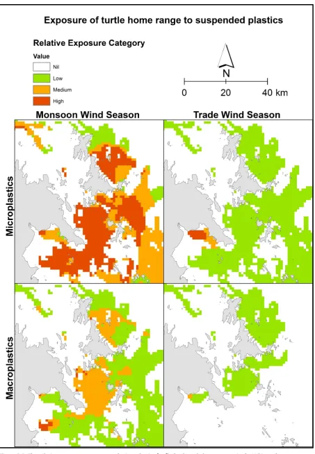
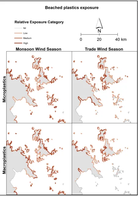
iii based on the density of particles in modelling outputs of nil, low, medium and high exposure. I found that in the trade wind season (April to September, dominated by strong south-easterly winds) marine turtles, mangroves and reef habitats had lower exposure than during the monsoon wind season (October to March, dominated by lighter and more variable winds). A small proportion of coral reef habitat was in the high exposure categories, whereas the turtle home-range had a large area in high exposure categories (16% and 26% exposed to high microplastics during monsoon season, respectively). Unlike the other two case studies, the mangrove habitat had consistent hotspots of high exposure across both wind seasons. The outputs of this chapter can inform local scale management action, for example turtle management and recovery plans. The method presented here can also be transferred to other species and habitats and scaled up for larger jurisdictions.

In the third data chapter, I built on Chapter 2 (a sensitivity analysis of physical/modelled processes) by using field data for macro- and microplastics to interrogate the model. The aim was to find the likely sources of plastics to the Whitsunday region and understand the limitations for the model in a complex coastline and at a management-relevant scale. I found that, for microplastics, offshore sources are likely to be more important than onshore, and for macroplastics, local (onshore) sources are more important than they are for microplastics. Of the physical characteristics I examined, I found none that make a site more or less predictable in the modelling. Field data on sources at local scales is necessary, although, this is recognised as a difficult task.

iv

v I would first like to acknowledge the external funding that I received from the Great Barrier Reef Marathon fund and the Australasian Hydrographic Society. I also received a donation of plastics for my experiments by Robert Dvorak at Visy Plastics. Llew Rintoul and John Colwell provided technical support. Eric Nordberg donated elastomer. My experiments would have been significantly more difficult without the help, advice and support from the MARFU Technicians, Simon, Andrew and Ben. I also appreciate the practical help, advice and resources I received from Giverny Rodgers, fish master.

My fieldwork would have fallen flat without Dave Edge the barge driver in shining armour, and all around legend from Dave Edge Marine Contracting Pty Ltd. As well as my wonderful field volunteers - Harold, Alanna, Tess, Nicole, Annie and Michael. They didn’t moan about early mornings or “challenging” boating conditions. The data, time and support provided by Libby and the team from Eco Barge Clean Seas Inc. was invaluable to me and my project; another fieldwork saver. I also had help to process samples in the lab from Tiffany, Jay, Mimi, Rebecca and Edith, you were wonderful.

I am very fortunate to be surrounded by a diverse advisory panel. Firstly, Mark Hamann shares my passion for research towards action on plastic pollution and reminded me always to keep balance and perspective in all aspects of my life. Alana Grech believed in my abilities and showed me that a woman can be a successful scientist, a mother, and a great human being all at once. Mia Hoogenboom was my research rock, always encouraging me to think logically and push my horizons with scientific integrity at the centre of my science. She is balanced, calm, and kind - all things that I hope to emulate throughout my life and career. Lastly, Eric Wolanski, who never lost faith in me, always had my best interests in mind, and encouraged me to follow the science. I cannot thank you all enough. My thesis would have been much less than it is without all of your unique views.

I would also like to thank my collaborator Jonathan Lambrechts, he was a mentor and friend throughout my Honours and PhD theses.

vi

my microplastics friend, Annie, the very best write-up buddy, Kimmie, and others without titles, Natalie, Chris, Hector, Taka, and Astrid, thank you for all the coffee breaks and chats that helped me maintain perspective. To the coral physiology lab, led by Mia. Having access to people with different expertise was invaluable to me. Honourable mentions for Saskia, Tess, and Kath, and our lovely lunches, and Ally for all the help. It is not often you find colleagues that you can also call true friends. I am so lucky.

To my underwater hockey team, they don’t know how much they have helped me get through this experience with my sanity intact. Being able to escape was vital to my mental health. My dear friend and long suffering volunteer Sarah Hart, gave emotional support, practical help, and general awesomeness. My dearest Lexie Edwards, she is a wonderful helper and even better friend, I’m so lucky to have you and your family in my life. I arrived in Australia in late 2009, by the end of 2010 Denise and Lee Edwards had adopted me into their lives and family. There is no substitute for your parents, but Lee and Denise are as close as you can get - thank you for all your support, cups of tea, and hugs when all I wanted was to run away home. To my friends in far off places, it has been wonderful to have you there in the middle of the night, when I felt all alone.

My family, especially my Mum and Dad, although they are half the world away, they are always with me. My dad – you are a balancing force that few can disrupt and having your influence has been so valuable to my character. My mother – you truly understand me, we are cut from the same cloth, and I hope to one day be as strong, wise, and fearless as you. Your ongoing support and faith has meant the world to me, I’m so lucky that I get to call you both my parents. My brother, Ian, has been my best friend and protector since the day I was born - thank you for carrying the heavy things, and for all the food.

Lastly, Joshua, you are the family I choose and your support through time and distance has meant everything to me.

I could not have wished for a better group of people to have in my corner throughout this adventure.

vii Supervision

Associate Professor Mark Hamann, James Cook University Associate Professor Mia Hoogenboom, James Cook University Dr Alana Grech, James Cook University

viii

Field volunteers Annie Bauer-Civiello Michael Civiello Harold Cambert Nicole Rosser Alanna Kieffer Tessa Hill

Laboratory volunteers Tiffany Tsang

Jay Kim Mimi Hill Rebecca Anger Edith Shum

Statistical support

Rhondda Jones – Chapter5 Graphics support

Christine Wildermann – Chapter 2 Funding

Great Barrier Reef Marathon Fund Australasian Hydrographic society

James Cook University and the Australian Government for stipend and tuition fee support In-kind support

ix

co-authors

Chapter

Number Publication details Extent of the intellectual input of each author, including the candidate 2 Critchell K, Lambrechts J. Modelling

accumulation of marine plastics in the coastal zone; what are the dominant physical processes? Estuarine, Coastal and Shelf Science. 2016; 171:111-22.

I developed the research question. Lambrechts and I collected the data. I performed data analysis. I wrote the paper with input from editorial

Lambrechts. I developed the figures and tables.

3 Critchell K, Hamann M, Wildermann N, Grech A. A spatially explicit exposure analysis of plastic pollution in the Whitsunday region in prep

I developed the research question. Wildermann and I collected the data. I performed data analysis under the guidance of Grech. Wildermann

conducted home range analysis. I wrote the paper with editorial input from all. I developed the figures and tables under the guidance of Grech.

4 Critchell K, Hoogenboom M, Grech A, Wolanski E, Hamann M. Using field data to interrogate a plastics dispersal model in prep

I developed the research question. I collected the data. I performed data analysis under the guidance of Wolanski, Hamann, Grech and Hoogenboom. I wrote the paper with editorial input from all. I developed the figures and tables.

5 Critchell K, Hoogenboom M. Effects of microplastic exposure on the body condition and behaviour of

planktivorous reef fish (Acanthochromis polyacanthus) under review

Hoogenboom and I developed the research question. I conducted the experiment and data collection under the guidance of Hoogenboom. I performed the data analysis under the guidance of Hoogenboom. I wrote the paper with editorial input from Hoogenboom. I developed the figures and tables with support from

x

Permit approvals and ethics statement

xi

Table of Contents

List of publications associated with this thesis ... i

Abstract ... ii

Acknowledgements ... v

Statement of contributions ... vii

Publication plan with co-authors ... ix

Permit approvals and ethics statement ... x

Table of contents ... xi

List of tables... xiv

List of figures ... xv

Chapter 1 General Introduction ... 1

1.1 Risk assessment to inform management of plastic pollution ... 5

1.2 Dispersal of pollutants in the marine environment ... 9

1.5 Thesis objectives ... 14

Chapter 2 Modelling accumulation of marine plastics in the coastal zone; what are the dominant physical processes? ... 17

2.1 Introduction ... 18

2.2.1 The oceanographic model ... 21

2.2.2 The physical processes of drifting, beached and buried plastic ... 24

2.2.3 Data analysis ... 26

2.2.4 Ranking process ... 27

2.4 Discussion ... 38

Chapter 3 Predicting the exposure of coastal habitats to plastic pollution ... 43

3.1 Introduction ... 44

3.2 Methods ... 47

3.2.1 Study area and species ... 47

3.2.2 Hydrodynamic modelling and dispersal simulations ... 49

3.2.3 Exposure layers ... 52

3.2.3.1 Beached particles... 52

3.2.3.2 Suspended particles ... 53

3.2.3.3 Settled particles ... 53

3.2.4 Relative exposure categories ... 53

3.2.5 Habitat and organism distribution data ... 55

xii

3.3 Results ... 58

3.4 Discussion ... 68

Chapter 4 Using field data to interrogate a plastics dispersal model ... 73

4.1 Introduction ... 74

4.2 Methods ... 77

4.2.2 Overview of approach ... 77

4.2.3 Modelling scenarios ... 78

4.2.4 Microplastics field data ... 82

Site selection ... 82

Sample collection techniques ... 82

Processing sediment samples ... 84

4.2.5 Macroplastics field data ... 85

4.2.6 Comparison of model outputs to the field data ... 86

4.2.7 Site specific processes ... 86

4.2.8 Relative Exposure Index ... 87

4.3 Results ... 88

4.3.2 Microplastics Field data overview ... 88

4.3.3 Macroplastics field data overview ... 90

4.3.4 Source of the plastic to the region ... 90

Microplastics ... 90

Macroplastics ... 94

4.3.5 Non-source parameters ... 96

4.3.6 Characteristics of sites that influence prediction success for plastic accumulation ... 97

4.3.7 The site-specific processes that result in accumulation of macroplastics ... 99

4.4 Discussion ... 102

Chapter 5 Effects of microplastic exposure on the body condition and behaviour of planktivorous reef fish (Acanthochromis polyacanthus) ... 107

5.1 Introduction ... 108

5.2 Methods ... 111

5.2.1 Ethics Statement ... 111

5.2.2 Overview of approach ... 111

5.2.3 Preparation of microplastics ... 114

5.2.4 Acute exposure experiment – food replaced by plastic ... 114

5.2.5 Chronic exposure experiment – plastic dose added to normal food ... 114

5.2.6 Ontogenetic changes in sizes of microplastics ingested ... 115

xiii

5.3.1 Plastic ingestion ... 119

5.3.2 Growth and Body Condition ... 120

5.3.3 Behaviour... 122

5.4 Discussion ... 125

5.4.1 Behaviour ... 127

Chapter 6 General Discussion ... 129

6.1 Dispersal and accumulation of plastic pollution in the coastal zone ... 131

6.2 Risks of plastic pollution to the coastal zone ... 133

6.3 Implications for the management of plastic pollution ... 134

6.4 Key Limitations ... 137

6.5 Opportunities for future research ... 140

6.6 Concluding remarks ... 141

References ... 143

Appendix 1 ... 159

Appendix 2 ... 163

xiv

List of tables

Table 2.1: Parameters and values used in the sensitivity analyses ... 25

Table 2.2: Summary table of the indices for each scenario relative to the standard run (** the level of beached microplastics in this scenario is decreasing due to the rate of resuspension). The scenario numbers refer to the labels of Figure 2. 4 ... 28

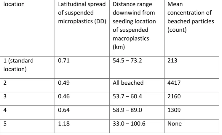
Table 2.3: Summary table of the comparative indices for each location scenario ... 31

Table 2.4: Average rank of each scenario and the rank of the process. The highest ranked scenario (rank 1) is the scenario that is most different from the standard run. ... 37

Table 3.1: Proven and speculated consequences of exposure to plastic pollution for each of the study habitats and species. ... 46

Table 3.2: The justification and importance of each source location in the plastic dispersal simulations. ... 51

Table 4.1: table of scenarios of modelled plastic movements. Columns show the values of each parameter used in each scenario and sources for these parameter estimates are described in Chapter 2. * shows the scenarios used in prioritising field sites. ... 81

Table 5.1: Summary table of statistical analyses. ... 124

A3.1 Table: Feeding regime for the chronic and acute exposure experiments ... 168

A3.2 Table: Feeding regime for the particle size experiment ... 168

A3.3 Table: Table of ANOVA results with the response variable initial weight ... 169

A3.4 Figure: Length weight relationships of the 3 clutches at the start of the experiment. ... 170

xv

Figure 1.1: Map showing the SLIM mesh across the model domain and at two scales of zoom (insets). ... 12

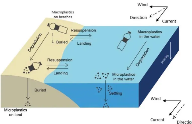
Figure 2.1: Schematic of the physical process pathways plastic items undergo when dumped at sea. ... 20

Figure 2.2: Case study area of the Whitsunday region of the Great Barrier Reef shown by the star in the inset map (a). Inset (b) shows an image of the simulation mesh around Hook Island in the Whitsunday group. The main map indicates the analysis area used to calculate the comparative indices and the seeding locations used for the simulations, Site 1 is the standard location. ... 23

Figure 2.3: Effect of seeding location on distribution of suspended and beached plastics after 8 days of simulation. The blue dots represent the macroplastics in suspension, the orange dots represent the microplastics in suspension and the purple represent the pooled macro- and microplastics that have landed on the beaches. The lower right panel shows the location of known hot spots for debris accumulation as described by Eco Barge Clean Seas Inc.

(personal communications 2013). ... 30

Figure 2.4: Concentration of beached (a) macroplastics and (b) microplastics, and location of (c) suspended and (d) settled macro- and microplastics, after 8 days for the ‘standard run’. ..32

Figure 2.5: The effect of degradation rate on particle locations after one month days at (a) 1x10-6 day-1 for plastics on the beach and 1x10-5 day-1 for plastics at sea. (b) 2x10-6 day-1 for plastics on the beach and 2x10-5 day-1 for plastics at sea. (c) 1x10-6 day-1 for beached particles, (d) 1x10-6 day-1 for plastics at sea. The star points represent microplastics, the dark circular points represent macroplastics and the seeding location is shown by the thick black cross. ... 34

Figure 2.6: The number of each particle type in the analysis area after days 1, 4 and 8 of simulation, for each scenario (the reader is referred to Table 2. 2 for scenario descriptions) each scenario was seeded with 10,000 macroplastics in suspension. ... 36

Figure 3.1: The Whitsunday region. The lower panel shows the placement of the hydrodynamic simulation seeding locations, shown as black circles. The river catchments are shown in green hues, with streams and rivers shown in grey. The top panel shows the placement of the region on the Queensland coast. ... 48

Figure 3.2: Wind rose of the wind data used in the modelling that created the exposure layers for each season, A) trade wind season and B) Monsoon wind season. Wind data from 10 min wind records at Shute Harbour weather station. ... 49

Figure 3.3: Example of the process used to create the relative exposure categories. The top panels show the process for suspended particles, whereas the bottom panels show the process for particles that have settled. The particles in this example are macroplastics in the Monsoon wind season. The particle locations were converted to a continuous grid via kernel density and then the quantile breaks used to split the data into four categories...54

Figure 3.4: Study area, the Whitsunday region. Top panel shows the locations of reef habitat in the study region, centre panel shows the home ranges of flatback turtles, and the bottom panel shows the coastline designated as Mangrove habitat. ... 56

Figure 3.12: Areas in each habitat that are in a consistent exposure category across wind seasons. ..67

Figure 4.1: Map showing the study area. Top panel shows the seeding locations used in the scenarios (black circles), the rivers (grey lines) and the catchment (green hues). The bottom panel shows the seeding locations used for the grid scenario. ... 80

Figure 4.2: Map showing the predicted accumulation for each scenario used in the field site selection. Sites selected for field sampling (black circles) were based on these three sets of

xvi

Figure 4.3: Number of plastics found at each of the sampling sites (top panel). Data presented in the bottom panel are the number of plastic particles per sample - boxplots present the median mid-line of the boxes, the 25th and 75th percentile (box limits) and the vertical lines represent the range. ...89

Figure 4.4: Mean debris loads from all collection visits to macroplastic debris removal sites. The mean debris load is depicted by the size of the red circle. ...90

Figure 4.5: The number of sites correctly categorised by each scenario. For each of the scenarios, the sites were re-categorised based on the median predicted accumulation value for that scenario. Higher than the median values were designated “predicted hotspots” and lower than the median values were classified to be “predicted coldspots”. ...92

Figure 4.6: Particle distributions for microplastics from land-based and marine sources during the February scenario. The left panel shows the plumes of the two broad source locations at the end of the February 45 day scenario, for microplastics. The right panel shows the fit of the observed and predicted accumulation values at the field sites, the y axis error bars represent the standard error and the x axis error bars show the 25th _{and 75}th _{quartiles of}

the daily predicted accumulation values through the simulation. ...93

Figure 4.7: The number of sites correctly predicted in each scenario. ...94

Figure 4.8: Particle distributions for macroplastics from land-based and marine sources for the February scenario. The left panel shows the plumes of the two general source locations at the end of the February scenario, for macroplastics. The right panel shows fit of the observed and predicted accumulation values at the field sites. ...95

Figure 4.9: Details of the grid seeding scenario: A) seeding locations used in this scenario, B) scatter plot showing the observed and predicted accumulation values of the microplastic scenario, and C) scatter plot of the observed and predicted accumulation per week of macroplastic scenario. In both scatter plots the y axis error bars represent the standard error and the x axis error bars show the 25th _{and 75}th _{quartiles of the daily predicted accumulation values}

through the simulation. ...97

Figure 4.10: The predictability of each microplastic field site (i.e. the ability to categorise the site as hot or coldspot correctly). The top panel shows the number of times each site is correctly categorised in any scenario and bottom panel shows the geographic spread of predictive success. Insets show case studies of sites with various success rates. Success categories are coloured Blue (“Good”) to Red (“Very Poor”) scale shown in the legend and in the graph. 98

Figure 4.11: The correlation between A) relative exposure index and the prediction success of each microplastic site, and B) the relative exposure index and the observed accumulation at each microplastic site...99

Figure 4.12: Prediction success of macroplastic sites, bar graph shows the number of times each site is correctly categorised in any scenario. The map shows the geographic spread of

predictive success. Success categories are coloured Blue (“Good”) to Red (“Very Poor”) scale shown in the legend and in the graph. ...100

Figure 4.13: The correlation between A) relative exposure index and the prediction success of each macroplastic site, and B) the relative exposure index and the observed accumulation at each macroplastic site...101

Figure 5.1: Experimental design for acute and chronic plastic exposure experiment.Concentrations shown are the mean concentrations for each treatment, as treatment was dependent on tank biomass. The design of the aquarium room showing aquaria and outflow filters. ..113

Figure 5.2: Set up of length (A) and weight (B) data collection. A) shows the camera, grid paper and lighting set up for taking images of the fish to length analysis, and B) shows a juvenile A. polyacanthus in a two litre beaker of aquarium water on a balance. C) shows an example of a photograph used to measure the length, the green elastomer tag can be seen. ...118

Figure 5.3: Plastic ingestion by sub-adult A. polyacanthus exposed to different plastic doses. Top panels (A-C) show proportion of fish per treatment and clutch which ingested plastics, and the lower panels (D-F) show the range of ingestion for fish per pooled treatment

xvii

Figure 5.5: Fish growth and body condition during the acute phase of the plastic exposure

experiment. Top panels (A-C) show the change in mass (g) relative to start mass during the acute exposure phase, for each clutch. The lower panels (D-F) show the change in length-weight relationship relative to the start of the acute exposure, for each clutch, denoted in the grey panel above each graph. ... 123

Figure 5.6: Fish growth and body condition (measured as HSI) during the chronic exposure phase of the experiment. The top panels (A-C) show the change in body mass relative to the start of the chronic exposure, for each clutch, denoted in the grey panel above each graph. The lower panels (D-F) show the body condition of the fish in the form of the Hepatosomatic Index in each treatment and clutch, denoted in the grey panel above each graph. ... 124

Chapter 1

2

Over recent decades, the increase in population, technological developments and urbanisation have increased pollution in the environment. Some of the earliest pollutants were coal ash, industrial waste and sewage in the mid-19th _{century, coinciding with the industrial} revolution. It was not until the 1950s that the environmental movement began taking action towards reducing pollution inputs with legislation for clean air the America and the UK (Air Pollution Control Act, 1955; Clean Air Act, 1956, respectively), among others. The use of many substances deemed to contribute to pollution is controlled by legislation or other policy instruments aiming to prevent or minimise environmental harm. The management of point source and diffuse source pollutants differ. For point source pollutants, the source is known and identifiable, therefore legislating to set maximum emission limits is relatively common. For example, limits are set to manage emissions of heavy metals or persistent organic pollutants (POPs) by various industrial sectors. Diffuse source pollutants are more difficult to legislate for, essentially because it is not possible to locate the source, or the use is wide-spread and thus there is no single source contributing to the pollution. Dichlorodiphenyltrichloroethane (DDT), for example, is a chemical which has been used extensively as an agricultural insecticide for many decades, and although it is still used in some parts of the world as a malaria control method, its use is illegal in most developed nations due to its impact on the environment (UNEP, 2002; van den Berg, 2009). Despite these regulations across the globe, our air, soil and water systems are all experiencing an increased presence of pollutants.

3 Europe, 2016). Of this, it is estimated that a third of the plastic production goes to single-use packaging products.

With the increase in production and dependency of plastic-based materials, it is inevitable that plastic will end up in the natural environment. Plastic products can end up in the environment through irresponsible disposal, such as littering, accidental leakage from land-fill, and inadvertent loss through municipal waste-water treatment. Streets and storm drains often flow directly into freshwater systems where the plastics they carry accumulate (Eerkes-Medrano et al., 2015; Anderson et al., 2016; Cable et al., 2017). From the freshwater systems, the plastics are often washed into coastal and oceanic environments and these have become some of the most infamous accumulation zones of plastics in the environment. Plastics can also be deposited directly into the ocean though dumping at sea from vessels or from lost or otherwise discarded fishing gear. It is impossible to know with certainty how much plastic is in the ocean, however, estimates range from 5.2 trillion pieces (Eriksen et al., 2014) to 15 to 51 trillion pieces (van Sebille et al., 2015). Wherever the true value lies, the plastic load is large and increasing. Indeed, Jambeck et al., (2015) estimate between 4-12 million tonnes of plastics enter the ocean from land-based sources every year. Australia contributes a relatively small amount to the global problem due to the small population (Jambeck et al., 2015), however, there are significant accumulation areas on beaches all around the coast (Hardesty et al., 2017).

Plastics in the environment break-up into smaller and smaller pieces primarily because the polymer bonds undergo photo-degradation in the presence of Ultra-Violet (UV) light. In the ocean, decreased temperatures, and UV light attenuation, increase the time for plastics to degrade when compared to on land. Degradation on intertidal/exposed areas can be quite rapid. Weinstein et al., (2016) found that fragmentation of high-density polyethylene, polypropylene, and extruded polystyrene started at eight weeks in field experiments at Charleston, SC, USA (320 North). As plastics break-up into smaller pieces we classify them into size classes. Microplastics are generally regarded to be those smaller than 5 mm but larger than 100 µm, and macroplastics that are those larger than 5 mm. These size definitions are most common, however, they are not the only definitions that have been used in the scientific literature (Andrady, 2011). Plastics can enter the marine environment as macro- or microplastics, but the most commonly recognised source of microplastics comes from degraded macroplastic (Andrady, 2011).

4

et al., 2007; Maximenko et al., 2015). Indeed, some of the most publicised accumulation zones are the ocean gyres, generally located close to the centre of each ocean basin and driven by large-scale currents (Lebreton et al., 2012). The high degree of dispersal also makes the quantification and removal of plastics particularly difficult, because the plastics can disperse great distances away from their source, and accumulation zones are often a considerable distance from land. Furthermore, plastic products take a long time to break-up completely, but through time the object loses identifying marks and features, and as it remains in the environment for long periods of time, completing many circulations of the ocean, the sources are difficult to determine.

The occurrence of negative interactions between plastics and the environment has been well documented (Derraik, 2002; Andrady, 2011; Wright et al., 2013b). There have been many studies describing the observations of negative interactions to species with plastic pollution (see reviews by Thompson et al., 2009, Andrady 2011, and Chae and An 2017). The interactions with organisms, especially marine megafauna, are especially well documented (Baulch and Perry, 2014; Nelms et al., 2016). Ingestion and entanglement are the most widely recognised threats to aquatic animals. Entanglement in lost or otherwise discarded fishing gear, rope and plastic sheeting can reduce the ability of the animal to feed, move and behave normally (Gregory, 2009; Vegter et al., 2014; Duncan et al., 2017). It is also widely recognised that entanglement can damage the animal’s flesh or amputate/decapitate through blood restriction (Gregory, 2009). Entanglement can also, in the case of air-breathing aquatic animals, cause the animal to drown by weighing it down, reducing the animal’s ability to swim to the surface (Vegter et al., 2014; Nelms et al., 2016; Duncan et al., 2017). Ingestion of plastic material can cause damage to the digestive tract (Parga, 2012; Baulch and Perry, 2014) through lesions, abrasions and digestive blockages. If plastic particles are ingested and not passed through, they can cause physical blockage of the tract, as the particles fill the stomach causing starvation by reducing the feeding stimulus and reducing stomach capacity (Ryan, 1988). Ingested plastics can also transfer toxic substances to the animal causing disruption of the endocrine system (Rochman et al., 2013; 2014). Plastic pollution can also cause damage to habitats through smothering, scouring (e.g. Uneputty and Evans, 1997; Donohue et al., 2001) and changed physical properties (e.g. sand permeability and thermal properties associated with microplastic accumulation (Carson et al., 2011). Buoyant plastic objects also act as a vector for invasive species as they can remain a float for far longer than natural objects, allowing infauna and epifauna to travel greater distances (Chae and An, 2017). These impacts to the environment clearly need addressing though management action.

5 scientific data to underpin initiatives to minimise environmental harm, the science needs to be undertaken at a scale relevant to their management jurisdiction. Essentially, managers require robust data to be relevant to the jurisdictional area and of adequate spatial and temporal resolution to enable action (Fleishman et al., 2011). For example, Sherman and van Sebille (2016) used modelling to find optimal equipment placement locations for microplastic removal at sea. Large-scale projects are useful, however, management intervention is most feasible at the local jurisdictional scale and thus there is a need to conduct data collection and analysis at these smaller, jurisdictionally relevant, spatial scales. In Australia, local councils (municipal) and state government agencies are responsible for waste management, litter prevention and clean-up activities. The benefit of local management (council) intervention is that plastics can be prevented from entering the marine ecosystems at the source (Willis et al., 2017). Prevention of input at the source is cheaper, more effective, and ultimately reduces the subsequent problems, which can’t be easily resolved (Eagle et al., 2016; Willis et al., 2017). Knowing which individual sources to target is difficult without some estimation of which sources contribute the most to the system and where the plastics go after being dispersed from those sources. On a larger, global scale this has been quantified, and Schmidt et al., (2017) estimate that 88-95% of global plastic pollution is entering the ocean from just 10 urban river systems. However, there have been no attempts to quantify this at a scale relevant to local management.

There are many knowledge gaps in the information needed to conduct robust spatially explicit assessments of plastic distribution at spatial scales relevant to management activities. The scale of management changes with each level of government, with the state having a much larger jurisdiction than local councils. On average, local government in coastal regions (local councils) in Queensland, Australia, are responsible for 366 km of coastline. Models of plastic distribution available in the literature (e.g. Yoon et al., 2010; Maximenko et al., 2012) provide approximately seven cells of data across the Queensland coastline, which is therefore inadequate for decision making at scales of local councils. Therefore, this thesis aims to provide data at a scale relevant to local council management area. To achieve this, the spatial scale of the model I use must represent local geographic features in a meaningful way and provide an accurate representation of the hydrodynamics of the area.

1.1 Risk assessment to inform management of plastic pollution

6

decisions, weighing up the likelihood and consequence of activities, events and actions (Bottrill et al., 2008). Risk assessments incorporate two quantifiable aspects: likelihood of exposure and consequence of exposure. Risk assessments can be general, where the risk is assessed broadly and the approach results in one value for the risk of the threat. This can be relevant for threats that do not have a spatial component, for example the probabilistic environmental risk assessment of nanomaterials presented by Coll et al., (2016), or those associated with risks to human safety in industrial settings. However, for threats that change concentration or abundance in space and time, for example changing concentration of a pollutant via dilution or the changing density of receptor organisms, this approach is less valid. In these cases, a spatial-based risk assessment is one mechanism that can be used, which provide a map of continuous risk values across a spatially explicit area allowing managers to make spatial-based decisions or designate priority areas for management action (Lahr and Kooistra, 2010). On a global scale, Halpern et al., (2008) assessed the cumulative impacts of anthropogenic activities (stressors) on the marine environment, showing that every area of ocean is impacted by at least one stressor, but despite this global exposure there are areas of relatively low impact. These data allow managers in particular areas to prioritise activities accordingly. However, the data could only be used at the jurisdictional scale of the assessment. To act at a state or local level this resolution would be inadequate.

The exposure of the threat is broken down into the distribution of the threat and the interaction rate with the chosen receptor, such as a habitat or species of animal. The distribution of the threat is often measured using field data and the values between observations are interpolated, or the distribution is modelled based on predictor variables. For example, Srivastava et al., (2012) used water quality field measures in a broader assessment of water quality in India. For pollutants that have fairly homogeneous distributions, or have transport mechanisms that are understood, this method works well. However, for a patchy, variable, and long-lived pollutant in the coastal environment, such as plastics (Barrows et al., 2016; Underwood et al., 2017), this method may be relevant for only the time stamp of field data collection. Collecting samples for marine plastics (especially microplastics) is time consuming and the processing of the samples can take considerable time. Therefore, field data for mapping the distribution of plastic-based pollution is often not feasible at the spatial resolution required for management, especially in areas removed from urban, coastal environments.

7 abundance data along with data on the habitats and the species abundance in the area. Indeed, Nelms et al., (2016) list the need to develop risk maps for sea turtles to be a key future research direction, citing interaction rates as a knowledge gap and suggesting use of oceanographic and niche models to improve knowledge. As an alternative method, Darmon et al., (2017) calculate the interaction rate between turtles and macroplastics in the Mediterranean using aerial survey techniques. They counted the amount of plastics found within a 2 km radius of a turtle to calculate the frequency of interactions. However, this technique would almost certainly be biased towards larger plastic items.

Understanding the consequences of pollutant-organism interactions is the final component of risk assessment. Consequence can be assessed in a few different ways (Lahr and Kooistra, 2010). For example, if concentration effects are known, the probability of an effect can be calculated. Lan et al., (2015) describe a framework for assessing the risk of oil spills that incorporates the impact of the oil and resilience. More simply, if a threshold value is known (e.g. LD50) this can be used to incorporate consequence into spatial risk assessments (Lahr and Kooistra, 2010). Many environmental risk assessments use implied consequence, in that the presence of the pollutant is used to indicate an impact. For example, Fox et al., (2016) use seabird density and oil spill prevalence to assess the risk of oil spills to sea birds on the Pacific Coast of Canada. However, without the consequence component it is likely that the risk is over-stated (Valdor et al., 2017).

8

The knowledge and understanding of the consequence of plastic interactions with ecological features is increasing. Indeed, a search in the Web of Science for publications with the topics “plastic” and “impact” shows that publication volume has increased from 356 in the year 2000 to 1587 in 2017 (also see Vegter et al., 2014; Nelms et al., 2016). Plastic particles of various sizes in the ocean or waterway expose animals to the threat of entanglement or ingestion. However, there is a lack of data on consequence that takes into account concentration effects of plastics on vulnerable species and habitats, especially in tropical regions. The number of species known to be impacted by plastic is large (Derraik, 2002; Andrady, 2011; Chae and An, 2017), and well documented in comparison to what is known about specific habitats, such as mangroves, seagrass, and coral reefs which have very limited data on the effect of the exposure to plastics. These knowledge gaps mean we don’t really understand risk of plastic pollution in the environment, especially with respect to its spatial accumulation.

9 pose to sea turtles. Even where the plastic/animal interaction takes place at a local jurisdictional scale, it is still poorly understood (Vegter et al., 2014; Nelms et al., 2015).

Managers need information in a reasonable timeframe to take timely, proactive management action. The time necessary to complete field sampling and sample processing over a jurisdictional area to capture the variability would mean the outcome would not be readily available for decision makers at the time the data are needed. A method that will provide robust data on distributions of plastics at an appropriate spatial and temporal scale, in a timeframe appropriate for management action, is therefore necessary for practical management application.

1.2 Dispersal of pollutants in the marine environment

As explained above, accurate quantification of the distribution of pollutants is a key component of the likelihood of an interaction that causes harm. In a spatial approach this would involve understanding where the threat is located in time and space. Gaining observation data of distributions is difficult especially in the marine environment because our oceans are large, homogenous and relatively inaccessible (Ban, 2009; Browne et al., 2011) in comparison to terrestrial systems. Consequently, marine field data are more expensive and time consuming to collect relative to the amount of data obtained.

There are many methods for tracking objects or water masses at sea, for example satellite imagery or hydrodynamic modelling. Satellite imagery is useful for remote applications and for collecting data over large geographic areas, and is often used in water quality monitoring and the study of ocean productivity (e.g. Harvey et al., 2015). However, if the object/substance does not have an irradiance signature, or is not in high enough concentration to produce a detectable irradiance signature, it has limited utility. To fill this gap, hydrodynamic modelling is an alternative approach to understand pollutant distributions and is inexpensive compared with field sampling but can still be used in remote environments (e.g. Andutta et al., 2012). There has been a rapid expansion in the use of modelling in scientific and industrial fields due to the ready accessibility of high-performance computing and the improved performance of personal computing, along with the accessibility of physical input data such as winds and tides (Peng, et al., 2013).

flood-10

plume modelling (Delandmeter et al., 2015). Modelling is also used for many ecological questions, for example turtle hatchling (Hamann et al., 2011; Wildermann et al., 2017) and larval dispersal (Andutta et al., 2012), and, of particular interest to my thesis, it is increasingly being used to understand the dispersal of plastic pollution (Yoon et al., 2010; Lebreton et al., 2012; Zhang, 2017).

Hydrodynamic models are inherently spatially explicit, and can be used to assess dispersal accumulation areas (or “hotspots”) of plastic pollution. However, most of the existing models used for plastic pollution examine patterns at large geographic scales, for example oceanic basins (Lebreton et al., 2012; Maximenko and Hafner, 2012; Reisser et al., 2013; Ebbesmeyer et al., 2007; also see review by Kubota et al., 2005), or at coarse resolution within regional seas (Kako et al., 2011 Pichel et al., 2012). To accurately predict areas of accumulation at a management-relevant scale, fine-scale spatial resolution is required (100s of meters to kilometres). However, the scales and resolution of existing models range from: whole ocean modelling with a coarse resolution of 0.5 degree (~56 km at the equator) (Yoon et al., 2010; Maximenko et al., 2012) to a single basin with a finer resolution of 1_{/12 degree (~9 km at the equator), for example, the East China Sea as in} Isobe et al., (2009) and the Coral Sea as in Maes and Blake (2015). The smallest scale of a single coastline, with variable resolution, was the Queensland Coast (Australia) in Critchell et al., (2015) and the Gulf of Mexico in Nixon and Barnea (2010).

It is now clear that, while studies at large scales are useful, modelling of plastics in the coastal zone at small scales needs to take into account not only the physical processes (wind and tide), but also the biochemical processes (e.g., biofouling and degradation) specific to plastics (Zhang, 2017). These processes are not included in many of the models described above, and the inclusion of plastic-specific processes into the modelling could vastly improve our ability to understand movements and accumulation. Many of the processes are not relevant at larger oceanic scales (e.g. island wind shadow), however, to model dispersal and accumulation at small scales, they must be taken into account. At smaller scales it becomes important to know the fine-scale water movements driving the movement of plastics and thus fine-fine-scale knowledge of processes are important. To model physical processes at this scale, a very fine resolution model is necessary. One such model is The Second-generation Louvain-la-Neuve Ice-ocean Model (SLIM; www.climate.be/slim).

12

of the Great Barrier Reef (20° S, 149° E) is in central Queensland, in the dry tropics region of the East Coast of Australia. Although the resident population is around 13,000 (Census, 2016), the region is one of the key tourism areas of the Great Barrier Reef and it receives around 500,000 tourists a year (National Visitor Statistics 2016). The Whitsunday area is important, economically and environmentally, therefore understanding the risk of plastics to this region will help managers prepare for future plastic abundance scenarios, e.g. calculating losses to tourism, and the necessity of intervention strategies.

The land associated with the Whitsunday region includes three main regional centres, Mackay, Proserpine and Airlie Beach. These regional centres are across two local council municipalities. The councils are responsible for waste management, and each council has independent waste management infrastructure making a combined management strategy for plastic pollution reduction in the Whitsunday region particularly challenging.

The region has two main seasons: Wet season (Monsoon Season, October to March), and the dry season (Trade Wind Season, April to September). The vast majority of the rain received in the region falls in the monsoon season, falling on three mainland river catchments; the Don (3690 km2_{), the Proserpine (2530 km}2_{), and the O’Connell (2390 km}2_).

Chapter 1: General Introduction

1.5 Thesis objectives

The goal of this thesis is to understand the dispersal and risks of plastic pollution at a local management relevant scale. Therefore, in this thesis, I use a multidisciplinary approach to gain new insight into all aspects involved in the risk of plastics. Specifically, I aim to: 1) understand the dominant processes involved in plastic movement and accumulation in the coastal zone; and 2) explore the risk of plastic exposure to vulnerable habitats and species in the tropical coastal zone. This thesis contains six chapters, with four data chapters, each of which address a specific objective towards the two aims described above. Chapters 2 and 5 have been published. The data chapters were written to serve as stand-alone papers but I have standardised the formatting to make a coherent body of work.

Chapter 1 - Provides background information and identifies specific knowledge gaps that the thesis aims to resolve.

Chapter 2 - Aims to understand the dominant physical processes involved in plastic movement and accumulation in the coastal zone. As noted above, existing hydrodynamic models of plastic dispersal exclude pertinent properties of plastics (e.g. degradation, resuspension from the coastline, and wind-drift), which may affect their dispersal and accumulation. In this chapter I introduce a plastic-specific hydrodynamic model and conduct a sensitivity analysis to explore the new processes included in the model. The sensitivity analysis I undertook aims to understand which of the processes have the most influence on plastic dispersal and accumulation.

Citation: Critchell, K. & Lambrechts, J., 2016. Modelling Accumulation of Marine Plastics in the Coastal Zone; What Are the Dominant Physical Processes? Estuarine, Coastal and Shelf Science 171, 111-122.

Chapter 3 - Aims to understand the risk of plastics to various vulnerable habitats and species in a spatially explicit approach to exposure. As noted above, the risks of plastics in the coastal environment are little understood, especially to determine where in the environment the risk is concentrated. In this chapter I use the new plastics model from Chapter 2 to create concentration distributions for plastics in the Whitsunday region and use these to inform spatial risk assessment for both habitats and species in the region, specifically coral reef, mangrove habitat, and flatback turtles.

15 Chapter 4 - Aims to use field data to interrogate the model in an attempt to further understand which hydrodynamic processes have the most influence on plastic dispersal and accumulation, at the small scale relevant to management, and to explore the sources of plastics in the Whitsunday region. This chapter builds on the knowledge gained in Chapter 2, which identifies the source of the plastics as the dominant key driver of accumulation hotspots. In this chapter I use field data for macro- and microplastics to compare with the model outputs of various modelled scenarios to understand the processes behind the observed accumulation.

Citation: Critchell, K., Hoogenboom, M., Grech, A., & Wolanski, E. & Hamann, M. in prep. Using field data to interrogate a plastics dispersal model.

Chapter 5 - Aims to understand the consequence of plastics exposure to marine life, using a planktivorous reef fish as a study species. I present the results of an experiment of microplastic exposure to the planktivorous reef fish Acanthochromis polyacanthus. The experiment: 1) explored the effect on body condition in the scenario of plastics replacing a natural food source; 2) assessed the scenario of microplastics in addition to food source; and 3) tested the amount of consumption at three plastic particle sizes for two size classes of fish.

Citation: Critchell, K. & Hoogenboom, M. under review. Effects of microplastic exposure on the body condition and behaviour of planktivorous reef fish (Acanthochromis polyacanthus)). PLOS One

Chapter 6 - Provides a synthesis of the thesis results, and discusses the limitations and implications of the work.

Chapter 2

Modelling accumulation of marine

plastics in the coastal zone; what are

the dominant physical processes?

Anthropogenic marine debris, mainly of plastic origin, is accumulating in estuarine and coastal environments around the world causing damage to fauna, flora and habitats (Chapter 1). Plastics also have the potential to accumulate in the food web, as well as causing economic losses to tourism and sea-going industries. If we are to manage this increasing threat, we must first understand where debris is accumulating and why these locations are different to others that do not accumulate large amounts of marine debris. This chapter demonstrates an advection-diffusion model that includes beaching, settling, resuspension/re-floating, degradation and topographic effects on the wind in nearshore waters to quantify the relative importance of these physical processes governing plastic debris accumulation. The aim of this chapter is to prioritise research that will improve modelling outputs in the future. I have found that the physical characteristic of the source location has by far the largest effect on the fate of the debris. The diffusivity, used to parameterise the sub-grid scale movements, and the relationship between debris resuspension/re-floating from beaches and the wind shadow created by high islands also has a dramatic impact on the modelling results. The rate of degradation of macroplastics into microplastics also has a large influence on the results of the modelling. The other processes presented (settling, wind-drift velocity) also help determine the fate of debris, but to a lesser degree. These findings may help prioritise research on physical processes that affect plastic accumulation, leading to more accurate modelling, and subsequently management in the future.

18

2.1 Introduction

The input and accumulation of anthropogenic marine debris such as plastics, is regarded in the public domain as an environmental and economic hazard. Macroplastic pollution (items larger than 5mm) accumulating on the coastline can affect tourism revenue (Jang et al., 2014) and the coastal habitat (Carson et al., 2011). The consumption of plastics, can cause damage to individual animals (Laist, 1997; Gregory, 2009; González Carman et al., 2014; Setälä et al., 2014) and have effects on the food chain (Boerger et al., 2010; Farrell and Nelson, 2013). There is evidence that microplastics (<5mm diameter) consumed by low trophic level species are transferred up the food chain as they are consumed by other trophic levels (Farrell and Nelson, 2013; Setälä et al., 2014). For these reasons it is important to create management action to prevent plastic waste from entering the environment, and there is a need to devise efficient debris removal schemes. While considering the importance of these factors, there are few data about the way different types of debris move in the ocean, why it accumulates in some locations more than others, and which parameters influence this most.

To maximise effectiveness of plastics debris removal for management and government agencies, geographic prioritisation of removal efforts must be considered. Oceanographic modelling is appropriate as part of a larger strategy to implement prioritisation and management (McElwee et al., 2012). The resolution required to accurately predict areas of accumulation at a beach scale is quite fine, ranging from a few 100 meters to 1 km. However, the recent models of plastic movement in the marine environment focus on models examining much larger scales, for example oceanic scales (Lebreton et al., 2012; Maximenko and Hafner, 2012; Reisser et al., 2013; Ebbesmeyer et al., 2007; also see review by Kubota et al., 2005), or within seas (Kako et al., 2011 Pichel et al., 2012) at coarse resolution. The scales and resolution of plastic movement models range from whole-ocean modelling with a coarse resolution of 0.5 degree (Yoon et al., 2010; Maximenko et al., 2012) to a single basin with a finer resolution of 1_{/12 degree i.e. the East China} Sea as in Isobe et al., (2009) and the Coral Sea as in Maes and Blake (2015). The smallest scale of a single coastline, with variable resolution was the Queensland Coast (Australia) in Critchell et al., (2015), and the Gulf of Mexico in Nixon and Barnea (2010). One reason for the large spatial scales is the time over which the simulations are run. The time scales varied from 30 years of simulations as in Lebreton et al., (2012) to a few weeks as in Carson et al., (2013) and Critchell et al., (2015).

19 al., (2011) modelled crab pots; and Isobe et al., (2014) studied different sizes of plastic and how they move in on-shore and off-shore directions. Many studies, however, continue to model plastics as a general category (Isobe et al., 2009; Martinez et al., 2009; Yoon et al., 2010; Hardesty and Wilcox, 2011; Kako et al., 2011; Lebreton et al., 2012; Maximenko and Hafner, 2012; Maximenko et al., 2012; Reisser et al., 2013; Maes and Blanke, 2015; Critchell et al., 2015).

Specialist, large-event debris models have also been developed. For example, the National Oceanic and Atmospheric Administration (NOAA) marine debris probability model developed for hurricane debris in the Gulf of Mexico, uses 100 m grid cells to compute probability of debris being found after a hurricane. Parameters such as wind speed, storm surge and infrastructure were used to assess the probability (Nixon and Barnea, 2010). A model for the debris from the 2011 Japanese Tsunami has also been developed by Maximenko et al., (2015), who used four different modelling systems with resolution from 1_/

4 to 1/12 of degree grid. The methodology used for oil spills has been found to be effective for modelling floating plastic debris (Le Hénaff et al., 2012), where the floating plastic is assumed to have a velocity equal to the vectoral sum of the water currents and the wind-drift velocities. The direct movement of plastics due to the wind (wind-drift) is neglected in many studies that model the movements of plastic in the ocean (Isobe et al., 2009; Martinez et al., 2009; Kako et al., 2011; Reisser et al., 2013; Isobe et al., 2014; Maes and Blanke, 2015). In studies that include wind-drift, the value of the wind-drift coefficient varies from 1% (Ebbesmeyer et al., 2011) to 6% (Maximenko et al., 2015), and in some studies a range of values are used or the value used is not given but instead the empirical formula for calculating the wind-drift is given (Kako et al., 2010). Submerged plastic debris is spread through the water column, with no exposure to the wind and hence no wind-drift is assumed (Reisser et al., 2013).

20

similar manner to oil-spill models for oil slicks. The oil-spill model methodology is basically advection-diffusion models coupled with chemical sub-models of the weathering of the oil, and are now routinely used by industry management (Chao et al., 2001; Tkalich et al., 2003; Guo and Wang, 2009). Such a model methodology is needed to improve predictions of debris accumulation and thereby improve management strategies for debris removal and mitigation. In addition, the improved model may also be used to backtrack and ultimately help to locate the sources of plastic pollution arriving at a given location, which would also support management goals (Reisser et al., 2013; Thiel et al., 2013). In order to work towards this, true values for the parameters described above must be experimentally determined or found through field observations.

In this study, I develop and explain a plastic oceanographic model to study the fate of plastics in estuarine and coastal waters (within 100 km of the coast). I demonstrate the application of this model in the complex case of a rugged coastal region with shallow waters and numerous islands and headlands. The basis of this plastics oceanographic model is a high resolution oceanographic, advection-diffusion model that also includes all the processes identified in Figure 2. 1. I propose a simple method to assess and rank the relative influence of these various physical processes on the movement of plastics in the coastal zone, using this method to prioritise research of the physical processes influencing plastic movements at sea.

21

2.2 Methods

2.2.1 The oceanographic model

To evaluate the relative importance of coastal processes on the movement of marine debris, I conducted a sensitivity analysis using the Second-generation Louvain-la-Neuve Ice-ocean Model (SLIM; www.climate.be/slim). SLIM is a depth-averaged, two-dimensional, finite element model with variable resolution developed by Lambrechts et al., (2008), which has been used for a variety of physical and ecological modelling tasks including: fine sediment, fish larvae, floating debris, and turtle hatchling dispersal (e.g. Lambrechts et al., 2008 and 2010; Hamann et al., 2011; Andutta et al., 2013; Critchell et al., 2015). The variable resolution (down to 100 m resolution) makes the model particularly useful in shallow coastal zones with complex bathymetry and topography. This model allows for fine-scale horizontal resolution and reduces the computational effort necessary to represent the whole model domain. The appropriate use of a depth-average model in shallow, vertically well-mixed waters was previously explored by Critchell et al., (2015). In that study, it was shown that, in well-mixed shallow water environments, the diffusion patterns of particles are very similar at the surface, middle and bottom of the water column, and the use of a three-dimensional modelling approach, (which is computationally very expensive) may be an unnecessary use of computational effort.

The study region used to conduct the sensitivity analyses was the Whitsunday region of the Queensland coast, and is part of the Great Barrier Reef Marine Park (20.20_{S, 149.0}0_{E; Figure 2.2).} This region is made up of approximately 74 coastal islands, coral reefs and other marine and coastal habitats. The coastal waters are primarily shallow with a mean depth <20 m (Figure 2.2). This region is also a tourism centre, making it economically important not only for Queensland but also for Australia as a whole. The area has had a marine debris removal program run by Eco-Barge Clean Seas Inc. since 2009. The islands and reefs create high levels of topographic and hydrodynamic complexity and create a large variety of unique locations with a rugged coastline, providing an ideal situation to quantify the relative importance of the various processes controlling the fate of plastics in complex topography and bathymetry.

22

in suspension, while not being directly be affected by the wind. A microplastic on the beach is assumed to be able to be resuspended. Simulation is discontinued for macro- or microplastics that have settled onto the sea floor and are assumed not to be resuspended (Figure 2.1). Simulation is also discontinued for macro- and microplastics that leave the model area through the open sea boundaries and are assumed not to be transported back into the study area. When the wind pushes either macro- or microplastic particles on a coastline, those particles are considered as beached. Beached particles do not move but have a chance to be resuspended/re-floated at each time step (5 minutes). Resuspended particles are placed at a random position in the neighbouring cell. In some scenarios, the resuspension rate is constant, in others beached particles in sheltered area (i.e. downwind coastlines) are assumed not to be resuspended.

24

2.2.2 The physical processes of drifting, beached and buried plastic

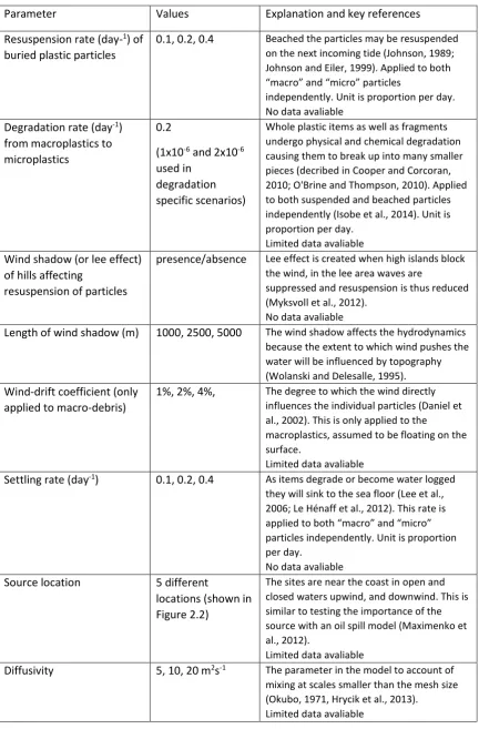
25 Table 2.1: Parameters and values used in the sensitivity analyses

Parameter Values Explanation and key references Resuspension rate (day-1_{) of}

buried plastic particles 0.1, 0.2, 0.4

Beached the particles may be resuspended on the next incoming tide (Johnson, 1989; Johnson and Eiler, 1999). Applied to both “macro” and “micro” particles

independently. Unit is proportion per day. No data avaliable

Degradation rate (day-1₎ from macroplastics to microplastics

0.2

(1x10-6 _{and 2x10}-6 used in

degradation specific scenarios)

Whole plastic items as well as fragments undergo physical and chemical degradation causing them to break up into many smaller pieces (decribed in Cooper and Corcoran, 2010; O'Brine and Thompson, 2010). Applied to both suspended and beached particles independently (Isobe et al., 2014). Unit is proportion per day.

Limited data avaliable Wind shadow (or lee effect)

of hills affecting

resuspension of particles

presence/absence Lee effect is created when high islands block the wind, in the lee area waves are

suppressed and resuspension is thus reduced (Myksvoll et al., 2012).

No data avaliable

Length of wind shadow (m) 1000, 2500, 5000 The wind shadow affects the hydrodynamics because the extent to which wind pushes the water will be influenced by topography (Wolanski and Delesalle, 1995). Wind-drift coefficient (only

applied to macro-debris) 1%, 2%, 4%,

The degree to which the wind directly influences the individual particles (Daniel et al., 2002). This is only applied to the

macroplastics, assumed to be floating on the surface.

Limited data avaliable

Settling rate (day-1_{) 0.1, 0.2, 0.4 As items degrade or become water logged} they will sink to the sea floor (Lee et al., 2006; Le Hénaff et al., 2012). This rate is applied to both “macro” and “micro” particles independently. Unit is proportion per day.

No data avaliable Source location 5 different

locations (shown in Figure 2.2)

The sites are near the coast in open and closed waters upwind, and downwind. This is similar to testing the importance of the source with an oil spill model (Maximenko et al., 2012).

Limited data avaliable

Diffusivity 5, 10, 20 m2_s-1 _{The parameter in the model to account of} mixing at scales smaller than the mesh size (Okubo, 1971, Hrycik et al., 2013).

26

To assess the effect of the seeding location on the results of the simulation, I used the standard parameter values from 4 more seeding locations. Site 1 (the standard location) and Site 4 were close to the coast on the lee side of the land, Sites 2 and 3 were on the exposed side of the land and close to the coast, and Site 5 was off shore, not affected by wind shadow (Figure 2.3).

2.2.3 Data analysis

For the scenarios examining the physical processes, the calculated latitude and longitude locations of the simulated plastics were extracted for each day of simulation using an analysis area around the source location (see Figure 2.2). The analysis area was set around the seeding location so that the edge of the analysis area was close to the coast, this was to reduce the area that would be impossible for simulated plastics to be in. The plastic particles (macro: beached, floating on the surface, settled, and micro: beached, suspended in the water column, settled) that remained in the analysis area (Figure 2.2) were used to create indices to compare the different scenarios through time. All the scenarios examining the physical processes were seeded from the standard location, within the analysis box. The scenarios assessing the effect of seeding location were compared using different indices, which did not use the analysis box, described later.

The following indices were calculated for each of the physical process scenarios: (1) residence time (days) of suspended macroplastics, to be able to compare the rate at which they leave the system; (2) residence time of beached macroplastics, to compare the time spent on the coastline in macroplastic state; (3) time for doubling (days) of microplastics on the beaches, using the number of microplastic particles on the beach by the end of day 1 as the starting value to evaluate the rate of increase of microplastic particles; (4) maximum number of suspended microplastics in the study area after initial release, to understand the change from the standard in settlement, resuspension, and drifting from the analysis area; (5) total accumulated macroplastics on the sea floor; and (6) total accumulated microplastics on the sea floor. These parameters were used to understand the rate of accumulation over the 8 day simulati