Accepted Manuscript
Research papers
Predicting Water Allocation Trade Prices Using a Hybrid Artificial Neural Net-work-Bayesian Modelling Approach
Tai Nguyen-ky, Shahbaz Mushtaq, Adam Loch, Kate Reardon-Smith, Duc-Anh An-Vo, Duc Ngo-Cong, Thanh Tran-Cong
PII: S0022-1694(17)30814-4
DOI: https://doi.org/10.1016/j.jhydrol.2017.11.049
Reference: HYDROL 22407
To appear in: Journal of Hydrology
Received Date: 11 September 2017 Revised Date: 25 November 2017 Accepted Date: 27 November 2017
Please cite this article as: Nguyen-ky, T., Mushtaq, S., Loch, A., Reardon-Smith, K., An-Vo, D-A., Ngo-Cong, D., Tran-Cong, T., Predicting Water Allocation Trade Prices Using a Hybrid Artificial Neural Network-Bayesian Modelling Approach, Journal of Hydrology (2017), doi: https://doi.org/10.1016/j.jhydrol.2017.11.049
PREDICTING WATER ALLOCATION TRADE PRICES USING A HYBRID
ARTIFICIAL NEURAL NETWORK-BAYESIAN MODELLING APPROACH
TAI NGUYEN-KY1*,SHAHBAZ MUSHTAQ2,ADAM LOCH3,KATE REARDON-SMITH2,
DUC-ANH AN-VO1,DUC NGO-CONG1 AND THANH TRAN-CONG1
1
Computational Engineering and Science Research Centre (CESRC), University of Southern Queensland, Toowoomba, Qld 4350, Australia
2
International Centre for Applied Climate Sciences (ICACS), University of Southern Queensland, Toowoomba, Qld 4350, Australia
3
Centre for Global Food and Resources, University of Adelaide, South Australia 5005 Australia
Key Points
• Artificial Neural Network (ANN) approaches were used to model and predict water trading prices in the Murry Irrigation area, Australia.
• Prices forecast using hybrid ANN-Bayesian modelling showed greater agreement with actual water prices.
• Water security allocations, cereal and meat prices were significant determinants of future water trading prices.
Abstract: This paper proposes an integrated (hybrid) Artificial Neural Network-Bayesian (ANN-B)
modelling approach to improve the accuracy of predicting seasonal water allocation prices in Australia’s Murry Irrigation Area, which is part of one of the world’s largest interconnected water markets. Three models (basic, intermediate and full), accommodating different levels of data availability, were considered. Data were analyzed using both ANN and hybrid ANN-B approaches. Using the ANN-B modelling approach, which can simulate complex and non-linear processes, water allocation prices were predicted with a high degree of accuracy (RBASIC = 0.93, RINTER.= 0.96 and RFULL = 0.99); this was a higher level of accuracy than realized using ANN. This approach can potentially be integrated with online data systems to predict water allocation prices, enable better water allocation trade decisions, and improve the productivity and profitability of irrigated agriculture.
Keywords: Water allocation prices, Artificial Neural Network model, hybrid Artificial Neural
Network-Bayesian model, water trade, price prediction. _____________
2 1. Introduction
Existing irrigated agriculture will come under intense pressure due to shifts in weather patterns, changes in rainfall events and increasingly varied hydrological regimes (IPCC, 2012). These changes will cause increased agricultural water demand, especially during dry years. Most farm water use and management decisions are based on seasonal water allocations and the opportunity cost of water use (Randall, 1981). Water markets, where they exist, provide farmers with clear opportunity cost and price signals that can potentially improve the economic efficiency of water use in terms of higher profit per hectare and per megalitre of water, given limited water availability and higher inter-temporal risk (Qureshi et al., 2010, 2013). This is because, in the absence of distortions, water markets allocate water to equalize the marginal benefits from its use across sectors/users and to magnify social welfare (Skurray, 2012). A perfectly competitive market, in equilibrium, will result in water prices equal to the value of its marginal product, while water prices generated under distortionary (e.g. political, institutional, infrastructural, informational) constraints may result in inefficient resource use at the margins (Chong et al., 2006). Access to water markets can also assist agricultural water users in their adjustment to uncertainty through participation in water allocation trade, consistent with their risk management and commodity options (Brennan, 2004). Thus, improved water allocation price information may lead to more efficient use of increasingly scarce and expensive water resources, resulting in increased farmer returns on investment and positive social welfare outcomes.
Sates, for example, prices can be driven by the volume of water allocations traded between urban and agricultural users (Colby et al. 1993); although since >95% of water trades in Australia are agricultural in nature this may be of lesser concern (Bjornlund and Rossini 2007). Important drivers of Australian water allocation trade prices typically include: water scarcity (abundance) as a consequence of drought (flooding) events which also impact on rainfall and evaporation variations (Bjornlund 2004; Bjornlund and Rossini 2005); seasonal allocation announcements on the back of annual rainfall outcomes and water manager assessments (Bjornlund 2002, 2003; Peterson et al. 2004; Brennan 2006); risk averse attitudes held by farmers or different industries (Brennan 2006; Brooks and Harris 2008); the substitutability of water for other farming inputs such as feed (Bjornlund 2003; Peterson et al. 2004); spatial or physical trade restrictions within and between different areas (Gardner and Miller 1983; Brennan 2006); inefficient trade rule and/or price discovery processes (Brennan 2006); cost-differences between water allocation and other trade products (Brooks and Harris 2008); the degree to which water is required to preserve capital-intensive production systems (Bjornlund and Rossini 2005; Adamson et al. 2017); and the bargaining strength of different traders in the market (Gardner and Miller 1983) or the presence of strategic bidding behaviour in the form of excessive demand variability (Oczkowski 2005).
4
premium early in a season to reflect supply uncertainty and a risk premium above the expected water value, which would be likely to decline monthly over the season as a rule (Brennan 2006). So if the capacity of different water users to forecast allocation water prices can be improved, this may increase their respective gains from trade (and/or decrease the risk premiums incurred) by irrigators over the course of a season.
1.1 The value of water allocation price predicting
6
While the benefits of improved water allocation demand (price) predicting accuracy may be mixed depending on an agricultural water users’ operation and accuracy requirements (Zareipour et al., 2010), improved capacity by agricultural water users to make timely annual selections of annual commodities and/or adopt risk management arrangements with more accurate water allocation price predictions should create economic welfare and improved marginal water use outcomes (Dziegielewski, 2011). Further, the provision of effective information and institutional platforms to support water allocation price prediction has not matched market development (Wheeler, 2016; Wheeler et al., 2017; Cui and Schreider, 2009); this is particularly critical given the monthly price variation typically evident in water allocation price reporting (e.g. National Water Commission, 2013).
1.2 Prediction approaches
Predicting water allocation prices faces significant challenges due to the complexity of the relationships involved. Typically, water resource researchers have used conventional modelling techniques such as regression analysis, time series analysis and autoregressive moving averages (Jain
system (Lawrence, 1997; Smith and Mason, 1997; Khan et al., 2010). Neural networks are non-linear parallel computational techniques which are flexible and offer better fitting outputs with regard to the training data, than linear models. However, an error of over-fitting can occur during neural network training with a large number of parameters in the new data (Srivastava et al. 2014).
Bayesian approaches, based on Bayes’ rule, incorporate a likelihood function, which calculates the probability of the observed data conditional on the values of other parameters in the dataset (MacKay, 1992; Robert, 2007). Hence, a hybrid ANN-Bayesian modelling approach should enable a more probabilistic interpretation of the behaviour of a complex dataset. Kingston et al. (2005) used a Bayesian model selection (BMS) method based on Markov Chain Monte Carlo (MCMC) approach applied to a salinity forecasting case study. In contrast to a solely neural network model, the ANN-B model can solve the over-fitting problem using Bayesian regularization (MacKay, 1992). Ideally, the network training algorithm will adopt a Bayesian regularization back-propagation approach to update the weight and bias values according to Levenberg-Marquardt optimization.
anticipate water allocation prices across the cropping season; this information can be used in decision-making to potentially improve the gains from trade.
2. Methods
2.1 Study area
The study area for the paper is the Murray Irrigation Area (MIA), located in the southern MDB (Figure 1). Irrigation farming activity in this region accounts for 7.7% of total MDB irrigation water use (MIL, 2006). The land-use pattern in the Murray Irrigation Area shows the diverse nature of agriculture in the region (see supplementary Table S1). In the MIA, the average level of allocation made against general security entitlements1 was about 124% before restrictions on water extraction were imposed in 1994–95 with the imposition of ‘the Cap’2, falling to 65% after this (see supplementary Figure S1). The region has an annual bulk water entitlement of 1,479,000ML (see supplementary Table S2) and is generally a net importer of water facilitated through the water market. The local privately-owned irrigation company, Murray Irrigation Limited (MIL), provides water from their bulk holding to about 2,416 landholdings (total land area of 748,000 ha), as well as urban water supply to eight local rural towns.
1 General Security water entitlements are a lower-reliability product that may deliver an allocation in, for
example, 50% of years subject to water demand/availability circumstances.
2 The ‘Cap’ was a limit on total water extractions from the MDB that was first trialled (1994–95), and later fully
Figure 1: Murray Irrigation Area, Australia. (Source: http://www.murrayirrigation.com.au/).
Markets for water have a lengthy history in Australia, and are now reasonably well established in the southern MDB (Loch et al., 2013). Relatively low transaction costs associated with water allocation trade mean that markets provide a useful risk-mitigation strategy for MDB irrigators, particularly during droughts (Wittwer and Griffith, 2011). Since 1994–95, when the Murray Darling Basin Commission imposed the Cap limit on total water diversions, water trading activity has gradually increased. The volume of water traded throughout the MIA has also risen steadily in response to periodic variations in seasonal water volumetric allocations. For instance, at the height of the Millennium Drought, some 95,000ML of water allocations worth AU$4.3 million was traded between August 2005 and May 2009 (MIL, 2006), and decreases in agricultural production and net income were lower than expected under the counterfactual, highlighting the value of water trade (Wittwer and Griffith, 2011).
2.2. Analytical framework
10
Three models are proposed to forecast water allocation prices; these are referred to as the basic, intermediate and full models (Khan et al., 2010) described below:
(i) Basic model is designed with the weighted average price (A$ ML-1) of water allocations
from the current month to 3 months earlier, as follows:
(
w w)
w
f
P
P
P
T(m+1)=
T(Avg.(m,m−1,m−2),
T(Avg.(m−1,m−2,m−3)) (1)(ii) Intermediate model is based on the weighted average price (A$ ML-1) of water
allocations, the average Standardized Precipitation Index (SPI) (McKee et al., 1993) and the average general security water volumetric allocation (percent) from the current month to four months earlier:
= − − − − − − − − − − − − − − − − +
A
A
A
SPI
P
P
f
P
T m m m Avg T m m m Avg T m m m Avg T m m m Avg T m m m Avg T m m m Avg T m w w w ) 4 , 3 , 2 .( ) 3 , 2 , 1 .( ) 2 , 1 , .( ) 3 , 2 , 1 .( )) 3 , 2 , 1 .( ( )) 2 , 1 , .( ( ) 1 ( , , , , , (2)In this model, drought is a more important factor, significantly impacting water allocation trade price and agricultural production over time. The SPI is used to determine the rarity of a drought at a given time scale for historic rainfall data.
(iii) Full model is designed for the current month and the previous two months based on the parameters in the intermediate model plus the weighted average prices of cereal crops (wheat, barley, sorghum, and rice), and meat (beef, lamb, and pork) which are the main agricultural outputs of the MIA:
M Month;
T Year;
Avg. Average;
Pw(m+1) Predicted water allocation price (A$ ML-1) for the next month;
Pw(Avg. (m, m-1, m-2)) Weighted average water allocation price (A$ ML-1) for the current month, last month and two months ago;
Pw(Avg. (m-1, m-2, m-3)) Weighted average water allocation price (A$ ML-1) for the last month, last two months, and three months ago;
SPI Avg. (m-1, m-2, m-3) Average standardized precipitation index (SPI) for the current month, last month and two months ago;
AAvg. (m, m-1, m-2) Average general security water volumetric allocation (percent) for the current month, last month and two months ago;
AAvg. (m-1, m-2, m-3) Average general security water volumetric allocation (percent) for the last month, two months ago and three months ago;
AAvg. (m-2, m-3,m-4) Average general security water volumetric allocation (percent) for two months ago, three months ago and four months ago;
Pc(Avg. (m, m-1, m-2)) Weighted average commodity price (A$ tonne-1) of cereal (c) crops for the current month, last month and two months ago (wheat, barley, sorghum, rice);
Pg(Avg. (m, m-1, m-2)) Weighted average grape (g) prices (A$ tonne-1) for the current month (m), last month and two months ago;
Pm(Avg. (m, m-1, m-2)) Weighted average meat (m) prices (cent kg-1) for the current month, last month and two months ago (beef, lamb, pork).
Descriptive statistics for all variables are presented in Table S3.
12
Time series data on water allocation trade covering the period from 1998 to 2015 were obtained from
the Water Exchange (the MIL water allocation trade platform) and various annual and environmental
reports from MIL (MIL, 2008–2015). Data for high and general security water volumetric allocation were obtained from MIL (2017) and the federal Department of Agriculture and Water Resources (2017).
Water use, and thereby water allocation demand, is a function of precipitation and evaporation, for which SPI—a normalized continuous rainfall variability function—is a proxy. The SPI was computed for four major regions in the study area (31.50S–360S, 143.70W–149.50W) from rainfall data for January 1999 to August 2015 obtained from the Australian Bureau of Meteorology (BOM, 2015). The index is based on statistical techniques and can quantify the degree of wetness and evaporation by comparing monthly rainfall totals with historical rainfall data (McKee et al., 1993). Data on commodity prices (see Supplementary Table S3) were obtained from the Australian Bureau of Agricultural and Resource Economics (ABARE, 2015).
Belsley collinearity diagnostics (Belsley et al. 1980) were used to assess the strength and sources of collinearity among variables in the multiple linear regression model; no significant correlations were identified.
2.4 Model Development: Hybrid Artificial Neural Network-Bayesian (ANN-B) modelling
Assuming the data are observations from a continuous probability distribution, the ANN-B model will begin by studying the distribution of the data in order to model their behaviour. According to the nature of ANN, the neural inputs are then processed by the likelihood function in Bayes’ rule. If the data are represented by X =(x1,x2,..., xn) and the set of parameters θ determines the probability
function L(θ |X) is then the probability of the observed data X conditional on the values of
parameter θ(MacKay, 1992; Robert, 2007):
∏
==
=
n i i nn
P
x
x
x
P
x
x
x
x
L
X
L
1 2 1 21
,
,...,
)
(
,
,...,
|
)
(
|
)
|
(
)
|
(
θ
θ
α
θ
θ
(4)The prior distribution P(θ) is defined to express the parameter
θ
. Suppose the input signalX
has thenormal observation | ~ ( , 2)
σ θ θ N
X , where standard deviation
σ
is known and the priordistribution for theta is
θ
~
N
(
µ
,
τ
2)
. The posterior distribution forθ
can be expanded via thenormal probability density function:
2 2 2 ) ( 2 1 ) , | ( τ µ θ π τ τ µ θ − − = e
f (5)
Bayes’ theorem gives the posterior probability density function (pdf) for parameter θas:
) ( ) ,..., , | ( ) ,..., , ( ) ( ) | ,..., , ( ) ,..., , |
( 1 2
2 1 2 1 2
1 α θ θ
θ θ
θ L x x x P
x x x P P x x x P x x x P n n n n = (6)
where P denotes the prior pdf of
θ
. The posterior distribution combines the prior function with the likelihood function (Figure 2).-500 -40 -30 -20 -10 0 10 20 30 40 50
[image:15.612.77.538.124.629.2]
14
Figure 2: Prior, likelihood and posterior density functions of the fluctuation of allocation trading
prices. Posterior probability is the product of prior probability and likelihood.
A Bayesian function can predict the value of an unknown quantity
x
n+1 with respect to the posteriordistribution of the parameters as:
∫
++
x
x
x
=
P
x
θ
P
θ
x
x
x
d
θ
x
P
(
n1|
1,
2,...,
n)
(
n1|
)
(
|
1,
2,...,
n)
(7)The objective of this model is to predict the distribution of the target values 1
+
n
y . The weights and
biases are trained, based on a set of the maximum of likelihood values for the input data
) ,..., ,
(x1 x2 xn
X = and associated targets
Y
=
(
y
1,
y
2,...,
y
n)
. From equation (6), the predicteddistribution of yˆn+1 can be presented as:
(
y+ x+ x y x y)
=∫P y+ x+ θ P(
θ x y x y)
dθP ˆn1| n1,( 1, 1),...,( n, n) (ˆn1| n1, ) |( 1, 1),...,( n, n) (8)
2.5 Model training and sensitivity analysis
When the network was trained, the divide function was automatically accessed and the data were randomly divided into three subsets. The fraction of data placed in the training set, validation set, and test set were as follows:
(i) a training set (train_ratio = 60%), used for computing the gradient and updating the network weights and biases;
(ii) a validation set (validation_ratio = 20%) in which the error on the validation set was monitored during the training process; and
The basic, intermediate and full model networks were trained through 1,000 iterations, where the mean squared error for both sub-samples decreased and then started to increase for the second/validation sub-sample, indicating that the network had learnt very effectively, conforming to the ANN and ANN-B primary principal of error minimization. When the training in Neural Networks was complete, the network performance could be used to check and determine if any changes needed to be made to the training process, the network architecture, or the data sets.
The models were also tested with regard to their sensitivity to the input variables (i.e. the relative impact of each input variable on water allocation price). Sensitivity analysis provided a key measure of the effect of an input value on the output value; hence, input variables with low sensitivity may be removed to decrease the network calculations as these will have little or no impact on the prediction result.
A nonlinear auto regressive model with an external input (ARX) was also used to predict the water allocation price over the time span of measured data to enable comparison and validation of the ANN and ANN-B models (Billings, 2013).
3. Results and Discussion
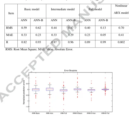
Table 1. Results for training, validation and testing of ANN and ANN-B models.
Item
Basic Model Intermediate Model Full Model
ANN ANN-B ANN ANN-B ANN ANN-B
Best-perf. 0.45 0.54 0.20 0.25 0.17 0.01
Best-vperf. 0.07 0.05 0.10 0.15 0.09 0.07
Best-tperf. 0.12 0.05 0.27 0.16 0.17 0.04
Perf. : performance; vperf.: validation performance; tperf.: testing performance.
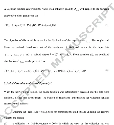
Figure 3 shows the value of the performance function versus the iteration number of training, validation, and test performance. The best network results for the ANN models were found at the 12th, 3th and 4th iterations for the basic, intermediate and full models, respectively (Fig. 3 a, b, c). For the ANN–B models, the best network results were found at the 4th iteration for the basic model, 4th iteration for intermediate model and at 5th iteration for the full model (Fig. 3 d, e, f). In these figures, there are no major problems with the training. Validation and test curves were similar, and no overfitting occurred.
Figure 3: Validation performance results for the ANN basic (a), intermediate (b) and full (c) models
[image:17.612.92.536.89.268.2] [image:17.612.76.537.413.676.2]3.1 Model validation
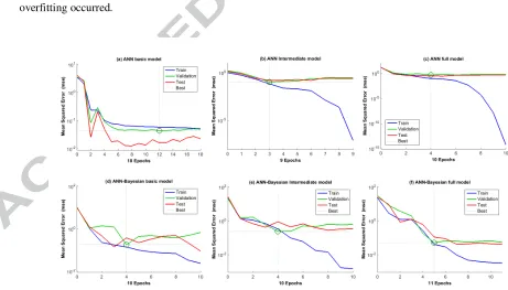
The validation of network performance was based on a regression of scatter plots of predicted versus observed water allocation trading prices, as shown in Figure 4. The regression coefficient (0≤R≤1)
[image:18.612.104.524.129.549.2]indicates the relationship between the actual water allocation price and the predicted water allocation price. The full ANN-B model showed better predicting performance, as reflected by the regression coefficients (RFull = 0.99) between actual and model generated water allocation prices, than either the intermediate (RInter.= 0.96) or basic (RBasic = 0.93) models. For the ANN model, regression coefficient values were RFull= 0.89, RInter.= 0.87 and RBasic= 0.82.
Figure 4: Regression of predicted water allocation price (network output) and the corresponding
observed water allocation price for the basic, intermediate and full ANN (a–c) and ANN-B (d–f) models. (The solid line shows the best linear fit and the dashed line shows the perfect fit.)
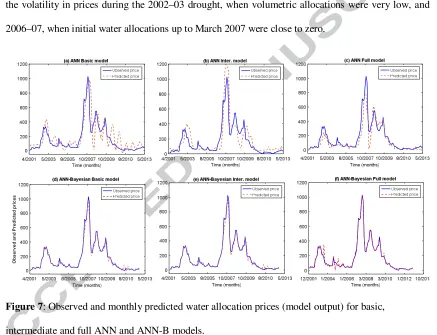
18
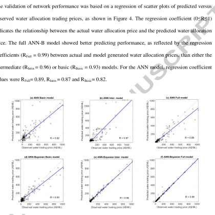
full ANN-B model is mainly associated with the inclusion of water volumetric allocations and cereal and meat prices, which enabled water allocation price volatility to be better captured than in other models, especially during the period between 2006–07 and March 2009, when water allocation prices
were very high due to extremely low seasonal water volumetric allocations in the MIL.
Figure 5: Time series responses for observed water allocation prices and predicted water allocation
prices of various models. (Time scale on the x-axis may vary because data were randomly
divided into three subsets when training the multilayer networks, as described in subsection
2.5)
3.2 Model testing
Overall, the models showed good predictive capabilities, with predicted water allocation prices close to actual water allocation prices in all six (basic, intermediate, and full ANN and ANN-B) models (Table 2). The full ANN-B model had the lowest minimum error, primarily due to the inclusion of more parameters than the basic or intermediate models. The full ANN-B model was also better able to forecast future water allocation prices with lower forecast error margins than the intermediate or basic ANN-B models across all months (Table 2, Figure 6). In all cases, the medians are roughly centered
E
rr
o
r
T
im
e
-s
e
ri
e
s
r
e
s
p
o
n
s
e
E
rr
o
r
T
im
e
-s
e
ri
e
s
r
e
s
p
o
n
s
[image:19.612.106.529.159.409.2]between the quartiles indicating that the middle half of the errors are roughly symmetric and the error distributions are not skewed.
A nonlinear auto regressive model with an external input (ARX) was also considered in the case of the full generic model for comparison (Billings, 2013). Predicting with ANN-B model gave better results than predicting with the ARX model.
Table 2. Model statistics for ANN and ANN-B basic, intermediate and full models used to predict
water allocation prices for September 1999 to May 2013 in the Murray Irrigation Area, Australia.
Item
Basic model Intermediate model Full model
Nonlinear ARX model
ANN ANN-B ANN ANN-B ANN ANN-B
RMS 0.59 0.62 0.44 0.47 0.40 0.13 0.70
MAE 0.33 0.23 0.33 0.29 0.23 0.05 0.41
R 0.82 0.93 0.87 0.96 0.89 0.99 0.802
RMS: Root Mean Square; MAE: Mean Absolute Error.
Figure 6: Error boxplots for the basic, intermediate and full ANN and ANN-B models.
ANN Basic ANN Inter. ANN Full ANN-B Basic ANN-B Inter. ANN-B Full -1.5
-1 -0.5 0 0.5 1
N
o
m
a
liz
e
d
p
re
d
ic
ti
o
n
e
rr
o
rs
[image:20.612.75.512.273.670.2]20
3.3 Predicting water allocation prices
[image:21.612.88.525.247.582.2]Network performance was assessed by comparing model outputs (prediction) with target (actual) water allocation prices in Figures 7(a, b, c) for ANN models, and 7(d, e, f) for ANN-B models. The ANN-B-model-generated predictions appear to more closely fit the actual data curves (Figure 7), indicating that, over the entire data set, ANN-B models show greater agreement between actual and predicted prices, and were therefore better able to predict prices. Overall, the full ANN-B model showed better prediction ability due to the inclusion of more parameters in the model which capture the volatility in prices during the 2002–03 drought, when volumetric allocations were very low, and 2006–07, when initial water allocations up to March 2007 were close to zero.
Figure 7: Observed and monthly predicted water allocation prices (model output) for basic,
intermediate and full ANN and ANN-B models.
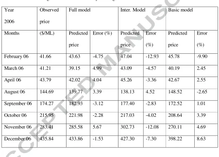
The results from the ANN-B Full, ANN-B Intermediate and ANN-B Basic models were tested by predicting water allocation prices. Table 3 shows the overall performance of the Basic, Intermediate and Full models in a real setting from February 2006 to December 2006, excluding winter months (May–July 2006) when there was little or no water allocation trading; this period was during the ‘Millennium drought’ (1996–2010) when water allocation prices were far higher than in previous
O
b
s
e
rv
e
d
a
n
d
P
re
d
ic
te
d
p
ri
c
e
[image:22.612.85.536.244.568.2]
years. The results from the ANN-B Full model has smaller errors than either the ANN-B Intermediate or ANN-B Basic models (Table 3); overall the error range (1.53%%–12.08%) highlights the superior capabilities of the ANN-B models.
Table 3: Observed prices, predicted prices and model errors for Basic, Intermediate and Full ANN-B
forecast water allocation prices for the eight month period from February to December 2006 during the Millennium Drought in Australia’s Murray-Darling Basin.
Year 2006
Observed price
Full model Inter. Model Basic model
Months ($/ML) Predicted price
Error (%) Predicted price
Error (%)
Predicted price
Error (%) February 06 41.66 43.63 -4.75 47.04 -12.93 45.78 -9.90
March 06 41.21 39.15 4.99 43.09 -4.57 40.19 2.45
April 06 43.79 42.02 4.04 45.26 -3.36 42.67 2.55
August 06 144.69 139.77 3.39 138.13 4.52 148.52 -2.65
September 06 174.27 182.93 -3.12 177.40 -2.83 172.52 1.01 October 06 215.95 221.98 -2.28 217.03 -4.02 208.64 3.39 November 06 283.41 285.58 5.67 302.73 -12.08 270.11 4.69
December 06 435.84 433.86 -1.53 427.30 -7.30 398.22 8.63
22
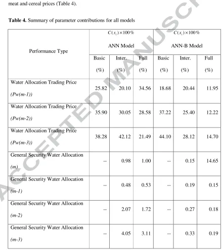
3.4 Network sensitivity
[image:23.612.77.516.221.717.2]Finally, we examined the sensitivity values of the model outputs to each input variable varied across input levels (Table 4). For example, water allocation prices were most influential in the basic, intermediate and full ANN models and in the basic and intermediate ANN-B models. However, meat and cereal prices were the most significant parameters impacting the predicted water allocation price in the full ANN-B model. The full ANN-B model was most sensitive to the water allocation price and meat and cereal prices (Table 4).
Table 4. Summary of parameter contributions for all models
Performance Type
% 100 ) (xi × C
ANN Model
% 100 ) (xi × C
ANN-B Model
Basic (%)
Inter. (%)
Full (%)
Basic (%)
Inter. (%)
Full (%)
Water Allocation Trading Price
(Pw(m-1))
25.82 20.10 34.56 18.68 20.44 11.95
Water Allocation Trading Price
(Pw(m-2))
35.90 30.05 28.58 37.22 25.40 12.22
Water Allocation Trading Price
(Pw(m-3))
38.28 42.12 21.49 44.10 28.12 14.70
General Security Water Allocation
(m)
-- 0.98 1.00 -- 0.15 14.65
General Security Water Allocation
(m-1)
-- 0.48 0.53 -- 0.19 0.15
General Security Water Allocation
(m-2)
-- 2.07 1.72 -- 0.27 0.18
General Security Water Allocation
(m-3)
Standard Precipitation Index (SPI) -- 0.15 0.05 -- 25.10 12.06
Cereal price (m)a -- -- 6.48 -- -- 14.78
Meat price (m)b
-- -- 2.48 -- -- 19.12
Total/constant 100 100 100 100 100 100
a
Cereal includes wheat, barley, sorghum and rice b
Meat includes beef, lamb and pork -- Not applicable
4. Conclusions and implications
Water scarcity is a key constraint to profitable agriculture. Water markets can reallocate water from low to high valued agricultural uses enabling gains in efficiency and overall productivity (White et al., 2006; Qureshi et al., 2013; An-Vo et al. 2015). In periods of scarcity, volumetric water allocations and water allocation prices will remain uncertain, hindering efficient decision-making regarding land and water management, investments into inputs, and potential national, regional and individual gains from trade. Continued drought can exacerbate this situation, and under such conditions water buyers and sellers will likely face high levels of water allocation price uncertainty in markets. The ability to forecast water allocation prices (e.g. seasonal allocation prices) could enable irrigators to make more informed decisions on water allocation and natural resource management to help boost returns to their investments by more effectively using increasingly scarce and expensive water supplies to gain from trade.
24
predicted (R=0.99) using an ANN-B approach, with simulation results from the ANN-B models found to be more accurate than those of the standard ANN models across a range of data inputs. The results indicate that current water allocation prices, general water security volumetric allocations and other data such as cereal and meat prices are significant determinants of future water allocation prices.
Application of the ANN-B model in a real world setting indicates the potential for good water allocation price prediction capability within the training range of the model. ANN-B models will be considered and improved for further commercialized applications such as spreadsheets and real time
data acquisition to enhance their functionality. The applications can also be useful for addressing a range of issues such as water allocation price risk, irrigation infrastructure investments and asset
management decisions; contingency planning for drought; natural resource management planning; and regional development planning. Further, the framework could be used to forecast volumetric allocations or water allocation prices in other irrigation districts to generate valuable information. With continued commitment by policy makers to the water allocation market, improved capacity of
agricultural water users in the timely selection of annual commodities and/or risk management arrangements with more accurate water allocation market price predicting in water markets should create greater economic and water use efficiency.
Acknowledgements
The support of the University of Southern Queensland’s Strategic Research Fund (SRF) is gratefully acknowledged. Funding from the Australian Research Council’s DECRA program (DE150100328) is also gratefully acknowledged by one of the authors.
ABARES, 2015. Commodity Statistics. Canberra ACT, Australia: Australian Bureau of Agricultural and Resource Economics and Sciences (ABARES). Available at: http://www.agriculture.gov.au/abares (accessed: December 2015).
Adamson, D., Loch, A. and Schwabe, K., 2017. Adaptation responses to increasing drought frequency. Australian Journal of Agricultural and Resource Economics 61(3), 385–403.
An-Vo, D.-A., Mushtaq, S., Nguyen-Ky, T., Bundschuh, J., Tran-Cong, T., Maraseni, T.N. and Reardon-Smith, K., 2015. Nonlinear optimisation using production functions to estimate economic benefit of conjunctive water use for multicrop production. Water Resources Management 29(7), 2153–2170.
Belsley, D.A., Kuh, E. and Welsh, R.E. (1980). Regression Diagnostics. New York NY, USA: John Wiley & Sons Inc.
Billings. S.A., 2013. Nonlinear System Identification: NARMAX Methods in the Time, Frequency, and
Spatio-Temporal Domains. Chichester, UK: Wiley.
Bjornlund, H. and Rossini, P., 2005. Fundamentals determining prices and activities in the market for water allocations. International Journal of Water Resources Development 21, 355–369.
Bjornlund, H. and Rossini, P., 2007. Fundamentals determining prices in the market for water entitlements-an Australian case study. International Journal of Water Resources Development 23(3), 537–553.
Bjornlund, H., 2003. What is driving activities in water markets? Water 30, 30–36.
Bjornlund, H., 2004. Formal and informal water markets: drivers of sustainable rural communities?
Water Resources Research 40(9), W09S07.
BoM, 2015. SILO Data. Melbourne Victoria, Australia: Government of Australia Bureau of Meteorology (BoM). Available at: http://www.bom.gov.au/ (accessed: December 2014).
26
Brennan, D., 2006. Water policy reform in Australia: lessons from the Victorian seasonal water market. Australian Journal of Agricultural and Resource Economics 50, 403–423.
Brennan, D., 2008. Missing markets for storage and the potential economic cost of expanding the spatial scope of water trade. Australian Journal of Agricultural and Resource Economics 52(4), 471– 485.
Brooks, R. and Harris, E., 2008. Efficiency gains from water markets: empirical analysis of Watermove in Australia. Agricultural Water Management 95, 391–399.
Cancelliere, A., Giuliano, G. Ancarani, A. and Rossi, G., 2002. A neural networks approach for deriving irrigation reservoir operating rules. Water Resources Management 16(1), 71–88.
Chong, H. and Sunding, D., 2006. Water markets and trading. Annual Review of Environment and
Resources 31, 239–264.
Colby, B.G., Crandall, K. and Bush, D.B., 1993. Water right transactions: market values and price dispersion. Water Resources Research 29(6), 1565–1572.
Cui, J. and Schreider, S., 2009. Modelling of pricing and market impacts for water options. Journal of
Hydrology 371, 31–41.
Department of Agriculture and Water Resources, 2017. Market price information for Murray–Darling Basin water entitlements. Canberra ACT, Australia: Department of Agriculture and Water Resources. Accessed (22 November, 2017) at: http://www.agriculture.gov.au/water/markets/market-price-information
Dziegielewski, B., 2011. Management of water demand: unresolved issues. Journal of Contemporary
Water Research and Education 114, 1.
Gardner, R.L. and Miller, T.A., 1983. Price behaviour in the water market of North-eastern Colorado.
Journal of the American Water Resources Association 19(4), 557–562.
Haykin, S., 1999. Neural Networks: A Comprehensive Foundation. 2nd Edition. Upper Saddle River NJ, USA: Prentice Hall.
IPCC, 2012. Managing the risks of extreme events and disasters to advance climate change adaptation: summary for policymakers. In: Field, C.B., Barros, V., Stocker, T.F., Qin, D., Dokken, D.J., Ebi, K.L., Mastrandrea, M.D., Mach, K.J., Plattner, G.-K., Allen, S.K., Tignor, M. and Midgley, P.M. (eds.) A Special Report of Working Groups I and II of the Intergovernmental Panel on Climate
Change. Cambridge, UK: Intergovernmental Panel on Climate Change (IPCC).
Horne, J., 2012. Economic approaches to water management in Australia. International Journal of
Water Resources Development 29(4), 526–543.
Jain, A., Varshney, A. K. and Johsi, U.C., 2001. Short-term water demand forecast modelling at IIT Kanpur using artificial neural networks. Water Resources Management 15(5), 299–321.
Khan, S., Dassanayake, D. and Rana, T., 2005. Ocean based water allocation forecasts using an artificial intelligence approach. In: Proceedings of MODSIM 2005 International Congress on
Modelling and Simulation Advances and Applications for Management and Decision Making.
Melbourne Vic., Australia (12–15 December 2005).
Khan, S., Mushtaq, S. and Chen, C., 2010. Waterworks: A Decision Support Tool for Irrigation Infrastructure Decisions at the Farm Level. Journal of Irrigation and Drainage Science 59(4), 404– 418.
Khan, S., Dassanayake, D., Mushtaq, S. and Hanjra, M.A., 2010. Predicting water allocations and trading prices to assist water markets. Irrigation and Drainage 59, 388–403.
Kingston, G.B., Lambert, M.F. and Maier, H.R., 2005. Bayesian training of artificial neural networks used for water resources modeling. Water Resources Research 41(12), W12409.
Kirby, M., Connor, J., Bark, R., Qureshi, E. and Keyworth, S., 2012. The economic impact of water reductions during the Millennium Drought in the Murray-Darling Basin. Australian Agricultural and
28
Lawrence, R., 1997. Using Neural Networks to Forecast Stock Market Prices. Winnipeg, Canada: Department of Computer Science, University of Manitoba.
Li, X., Maier, H.R. and Zecchin, A.C., 2015. Improved PMI-based input variable selection approach for artificial neural network and other data driven environmental and water resource models.
Environmental Modelling and Software 65, 15–29.
Liu, W.-C. and Chung, C.-E., 2014. Enhancing the predicting accuracy of the water stage using a physical-based model and an artificial neural network-genetic algorithm in a river system. Water 6, 1642–1661;
Loch, A., Bjornlund, H., Wheeler, S. and Connor, J., 2012. Allocation trade in Australia: a qualitative understanding of irrigator motives and behaviour. Australian Journal of Agricultural and Resource
Economics 56(1), 42–60.
Loch, A., Wheeler, S., Bjornlund, H., Beecham, S., Edwards, J., Zuo, A. and Shanahan, M., 2013. The role of water markets in climate change adaptation. Gold Coast QLD, Australia: National Climate Change Adaptation Research Facility (NCCARF).
MacKay, D.J.C., 1992. A practical Bayesian framework for backpropagation networks. Neural
Computation 4, 448–472.
Maier, H.R., Jain, A., Dandy, G.C. and Sudheer, K.P., 2010. Methods used for the development of neural networks for the prediction of water resource variables in river systems: current status and future directions. Environmental Modelling and Software 25(8), 891–909.
McKee, T.B., Doesken, N.J. and Kleist, J., 1993. The relation of drought frequency and duration to time scales. In: Proceedings of 8th Conference on Applied Climatology, American Meteorological
Society, January 17-23 1993 (Boston), pp. 179–184.
MIL, 2006. Murray Irrigation Sustainability Report. Deniliquin NSW, Australia: Murray Irrigation Limited (MIL).
MIL, 2017. Water. Deniliquin NSW, Australia: Murray Irrigation Limited (MIL). Accessed (22 November, 2017) at: http://www.murrayirrigation.com.au/water/
Mushtaq, S., Cockfield, G., White, N. and Jakeman, G., 2013. Modelling interactions between farm-level structural adjustment and a regional Economy: A Case of the Australian Rice industry.
Agricultural Systems 123, 34–42.
National Water Commission, 2010. The Impacts of Water Trading in the Southern Murray–Darling
Basin: An Economic, Social and Environmental Assessment. Canberra ACT, Australia: National
Water Commission (NWC).
National Water Commission, 2012. Water Policy and Climate Change in Australia. Canberra ACT, Australia: National Water Commission (NWC).
Nowlan, S.J. and Hinton, G.E., 1992. Simplifying neural networks by soft weight sharing. Neural
Computation 4, 173–193.
Oczkowski, E., 2005. Excess Demand, Market Power and Price Adjustment in Auction Clearinghouse
Markets for Water. Bathurst NSW, Australia: Charles Sturt University.
Peterson, D., Dwyer, G., Appels, D. and Fry, J., 2004. Modelling Water Trade in the Southern Murray-Darling Basin. Productivity Commission Staff Working Paper. Melbourne Vic., Australia: Productivity Commission.
Qureshi, M.E., Schwabe, K., Connor, J. and Kirby, M., 2010. Environmental water incentive policy and return flows. Water Resource Research 46(4), W04517.
Qureshi, M.E., Whitten, S.M., Mainuddin, M., Marvanek, S. and Elmahdi, A., 2013. A biophysical and economic model of agriculture and water in the Murray-Darling Basin, Australia. Environmental Modelling & Software 41, 98–106.
Randall, A., 1981. Property entitlements and pricing policies for a maturing water economy.
Australian Journal of Agricultural Economics 25(3), 195–220.
30
Sakaa, B., Chaffai, H. and Hani, A., 2013. The use of Artificial Neural Networks in the modeling of socioeconomic category of Integrated Water Resources Management (Case study: Saf-Saf River Basin, North East of Algeria). Arabian Journal of Geosciences 6(10), 3969–3978.
Skurray, J.H., Roberts, E.J. and Pannell, D.J., 2012. Hydrological challenges to groundwater trading: Lessons from south-west Western Australia. Journal of Hydrology 412–413, 256–268.
Smith, A.E. and Mason, A.K., 1997. Cost estimation predictive modeling: regression versus neural network. The Engineering Economist 42(2), 137–161.
Srivastava, N., Hinton, G., Krizhevsky, A., Sutskever, I. and Salakhutdinov, R., 2014. Dropout: a simple way to prevent neural networks from overfitting. Journal of Machine Learning Research 15, 1929–1958.
Wheeler, S., Bjornlund, H., Shanahan, M. and Zuo, A., 2008. Price elasticity of water allocation demand in the Goulburn-Murray irrigation district. Australian Journal of Agricultural and Resource
Economics 52, 37–55.
Wheeler, S., Bjornlund, H., Zuo, A. and Shanahan, M., 2010. The changing profile of water traders in the Goulburn-Murray Irrigation District, Australia. Agricultural Water Management 97(4), 1333– 1343.
Wheeler, S., Loch, A., Zuo, A. and Bjornlund, H., 2014. Reviewing the adoption and impact of water markets in the Murray-Darling Basin, Australia. Journal of Hydrology 518(Part A), 28–41.
Wheeler, S., 2016. Water Markets in the Murray-Darling Basin. In Griffin R. (ed.) Water Resource Economics: The Analysis of Scarcity, Policies, and Projects. 2nd edition. Cambridge Mass., USA: The MIT Press.
Wheeler, S., Loch, A., Crase, L., Young, M. and Grafton, R.Q., 2017. Developing a water market readiness assessment framework. Journal of Hydrology 552, 807–820.
Wittwer, G. and Griffith, M., 2011. Modelling drought and recovery in the southern Murray-Darling Basin. Australian Journal of Agricultural and Resource Economics 55, 342–359.
Wu, W., Dandy, G.C. and Maier, H.R., 2014. Protocol for developing ANN models and its application to the assessment of the quality of the ANN model development process in drinking water quality modelling. Environmental Modelling & Software 54, 108–127.
Zaman, A.M., Davidson, B. and Malano, H.M., 2005. Temporary water trading trends in Northern Victoria, Australia. Water Policy 7, 429–442.
32 Key Points
• Artificial Neural Network (ANN) approaches were used to model and
predict water trading prices in the Murry Irrigation area, Australia.
• Prices forecast using hybrid ANN-Bayesian modelling showed greater
agreement with actual water prices.
• Water security allocations, cereal and meat prices were significant