1
Optimal maintenance strategy for systems with two failure modes
Rui Penga, Bin Liub, Qingqing Zhaic*, Wenbin Wanga,d,aDonlinks School of Economics and Management, University of Science and Technology Beijing,
Beijing 100083, China.
bDepartment of Systems Engineering & Engineering Management, City University of Hong Kong,
Kowloon, Hong Kong.
cDepartment of Industrial and Systems Engineering, National University of Singapore, Singapore. dFaculty of Business and Law, Manchester Metropolitan University, UK.
*Corresponding author Phone: +65-94678450 Email: [email protected]
Abstract: This paper considers a single-unit system subject to two types of failures: a
traditional catastrophic failure and a two-stage delayed failure. Periodic inspections are
carried out to identify the defective stage of the two-stage failure process, whereas
preventive replacements are implemented to avoid any potential failure due to the
catastrophic failure mode. We construct a basic maintenance model and then extend it
to the cases of imperfect inspections (i.e., inspections that do not always notice a
defective state). We analyze the renewal process of the system and establish the
expected long-run cost rate (ELRCR). The optimal inspection period and preventive
replacement interval are determined by minimizing the ELRCR. A case study on
infusion pumps is presented to illustrate the proposed model.
Keywords: periodic inspection; preventive replacement; delay-time; two-stage failure
2
1.
Introduction
With the ongoing development of technology, modern systems are becoming
increasingly complicated and often have components that are subject to multiple failure
modes (Wang & Wu, 2014). In general, these failure modes can be classified into two
categories: hard failures and soft failures. Hard failures are the failures whose
occurrence is instantaneous and, most likely, self-announcing. Soft failures, on the
contrary, would generate early warning signals or have degradation patterns, which may
be detected by inspection or monitoring.
Modern complex systems, e.g., micro electromechanical systems (MEMS) and
complex medical devices, are usually subject to both hard failures and soft failures
(Park et al., 2013 and Peng et al., 2010). For instance, MEMS contain both mechanical
and electrical parts. The mechanical parts suffer wear that may be monitored or
inspected, whereas the electrical parts may fail suddenly and make inspections fruitless
for preventive maintenance. For complex medical devices such as infusion pumps, hard
failures can occur due to the malfunction of the alarm and circuit breaker/fuse, while
soft failures occur on the labeling and battery/charger. The voltage of the battery is
routinely checked, whereas the circuit breaker/fuse cannot be monitored and may
therefore fail suddenly.
To maintain a high availability, inspection is a commonly applied technique for
modern plant systems (Mendes et al., 2014 and Taghipour & Banjevic, 2012). Through
inspection, potential defects can be identified and preventive maintenance actions can
be carried out (Nguyen et al., 2015 and Wu et al., 2016). Accordingly, system failure
can be avoided and the operational cost of the system can be reduced. Thus, it is an
effective measure to improve the quality and performance of the system. Inspections
can be conducted periodically (Biswajit & Saren, 2016, Yang & Jae, 2014 and Liu et
3
or after the completion of successive tasks (Zhao & Nakagawa, 2013 and Liu et al.,
2016b). Periodic inspection is widely adopted in practice due to its easy implementation
and effectiveness. Wang (2009) formulated an inspection model with two kinds of
periodic inspection: minor inspection and major inspection. Aven and Castro (2009)
studied the optimal periodic inspection policy under safety constraints. Instead of
considering cost as the single objective, Ferreira et al. (2009) investigated the optimal
inspection interval in a multi-criteria framework.
Inspections are effective only if there are defective states for the system, so that the
system can be repaired preventively before a failure occurs. This leads to the usefulness
of the delay-time concept. Originally proposed by Christer (1976), the delay-time
concept regards the failure mechanism as a two-stage process, where the first stage is
from the installation to the point of a defect’s arrival and the second stage (known as
the delay-time stage) is from the start of the defective state to the failure, if left
unattended. This concept has inspired many subsequent studies, such as Christer (1999),
Wang (2012) and Zhao et al. (2015).Williams and Hirani (1997) studied the optimal
inspection policy for multi-state systems with multi-level maintenance based on the
delay-time model. Christer and Lee (2000) modified the delay-time model by
considering the downtime caused by failures. Wang (2011) extended the traditional
two-stage delay-time model to a three-stage process and studied the associated optimal
inspection policy. An overview of the recent delay-time-based maintenance models can
be seen in Wang (2012).
In practice, inspections can be imperfect due to the limitation of detection
techniques and the effect of environmental variations. An inspection may fail to identify
a defective state or mistakenly treat a normal state as the defective state (Biswajit &
Saren, 2016, Flage, 2014 and Phan & Zhu, 2015). Usually the performance of an
inspection is measured in terms of the probability of defect detection and the probability
4
inspection model and investigated the reliability of a system with a defective state. The
imperfect inspection model was further extended to the scenario of a finite horizon
(Berrade et al., 2013). Sheils et al. (2010) developed a two-stage inspection policy to
assess deteriorating infrastructure, in which the detection process is divided into two
stages: inspection and sizing. Mohammadi et al. (2015) integrated the imperfect
inspection model into a manufacturing system, where the optimal production period
and inspection policy were obtained. One limitation of the previous studies is that they
only consider one failure mode. In reality, a system is usually subject to multiple failure
modes (Liu et al., 2013 and Park et al., 2013). Imperfect inspection for a system with
multiple failure modes requires more investigation.
In this paper, we study the maintenance policy for a single-unit system subject to
two different failure modes. Failure mode 1 is the soft failure, and the failure process is
formulated using the delay-time model. Periodic inspections are conducted to detect the
possible defective state of failure mode 1. The case of imperfect inspection is also
considered by assuming that the probability of detection is constant. For failure mode
2, which belongs to the hard failure, the failure rate increases with the system age.
Preventive replacement is implemented to renew the system so as to decrease the
system failure rate. Appropriate preventive replacement policy is appreciated to balance
the failure probability and maintenance cost. To reduce the operational cost, the optimal
inspection and preventive replacement intervals that minimize the expected long-run
cost rate (ELRCR) are studied.
The remainder of this paper is organized as follows. Section 2 gives the detailed
system description and assumptions. Section 3 studies the basic model by assuming that
the inspection is perfect and the preventive replacement interval is an integer multiple
of the inspection interval. Different renewal scenarios are investigated in detail, and the
expected renewal cycle length together with the expected renewal cycle cost based on
5
imperfect inspections. Section 5 illustrates the proposed inspection and preventive
maintenance model with a case study on infusion pumps. Section 6 concludes the paper
and discusses possible directions for future study.
Notations
c
C Cost of a renewal cycle
F
C Cost of system failure
I
C Inspection cost
R
C Replacement cost
ECR Expected long-run cost rate
d
N Number of inspections to detect the defective state after the occurrence
of a defective state
T Periodic inspection interval
c
T Length of a renewal cycle
f
T Time of system failure
R
T Time to preventive replacement
1
X Duration of the system in normal state for failure mode 1
2
X Duration of the system in defective state for failure mode 1
3
X Duration of the system in operating state for failure mode 2
n Number of inspections before preventive replacement
Probability of defect detection
i
6
i
Scale parameter of Weibull distribution
2.
System description
The system under consideration is a single-unit system subject to two different,
independent failure modes. Both failure modes lead to the system failure. Failure mode
1 consists of a two-stage failure process, which is modeled using the delay-time concept.
With respect to mode 1, the system is first in the normal state, and then experiences a
defective stage prior to the eventual failure. The durations of the normal state and the
defective state are described by two independent random variables X1 and X2 ,
respectively. Denote the corresponding cumulative distribution functions (CDFs) as
( ), 1, 2
i
F i= , and the corresponding probability density functions (PDFs) as fi( ) .
Failure mode 2 corresponds to a hard failure, i.e., the failure occurs without any
prior warning, either because the defective state cannot be identified or there is no delay
time at all. The random time before failure for mode 2 is denoted by X3 . The
corresponding CDF and PDF are F3( ) and f3( ) , respectively.
To detect the possible defective state of failure mode 1, a periodic inspection of
period T is carried out during the operation of the system. The probability of defect
detection is assumed to be a constant (Williams & Hirani, 1997). Whenever the
defective state of failure mode 1 is detected, the system is immediately replaced. Since
failure mode 2 has no defective stage, inspection is ineffective. Nevertheless, to
mitigate the system failure due to mode 2, a preventive replacement is carried out at
R
T if no defective stage has been identified before TR. Whenever a failure occurs, it
can always be detected, and the system can be immediately renewed. Compared with
7
assumed to be negligible.
Let CI be the cost of a single inspection. We assume the cost of replacement at
inspections is equal to the preventive replacement cost at TR, which is denoted as CR.
When a failure occurs, corrective replacement is implemented to remedy the
consequences of the failure with the associated cost CF. Clearly, CF should satisfy
F R
C C . The cost items due to failure mode 1 and failure mode 2 are identical.
3.
The basic model
Before establishing the maintenance model, we investigate the stochastic behavior
of the system subject to two failure modes.
Consider failure mode 1 first. We have the CDF of failure mode 1 as
(
)
(
)
12( ) 1 2 1 , 2 1 0 1( ) 2( )
t
F t =P X +X =t P X t X −t X =
f F t− d .As failure mode 1 and failure mode 2 are independent, the CDF of the system lifetime
f
T can be obtained as
(
)
(
1 2 3)
(
12)(
3)
12 3 12 3
( ) 1 1 ( ) 1 ( )
( ) ( ) ( ) ( ).
f
F t P T t P X X t X t F t F t
F t F t F t F t
= = + = − − −
= + − (1)
With this result, we can proceed to formulate the maintenance model and further
analyze the effectiveness of the maintenance policy.
In this section, we assume that the inspection is perfect (=1 ) and that the
preventive replacement interval is an integer multiple of the inspection interval, i.e.,
R
T =nT, for integers n1. The system can be renewed in the following cases: (1) the
defective state of failure mode 1 is detected at the kth inspection, k =1,..., (n−1); (2) a
preventive replacement is carried out at nT ; and (3) failure occurs between
(
)
8
In the following, we first analyze these three possible scenarios and derive their
corresponding probabilities. Denote Tc as the length of a renewal cycle, and Cc as
the cost in a renewal cycle. The expected renewal cycle length E T( )c and the expected
renewal cost E C( c) can be obtained subsequently. Finally, the ELRCR, which is a
function of T and n, can be obtained as (Do et al, 2015; Wu et al, 2016) ( )
( , ) . ( )
c c
E C ECR T n
E T
= (2)
Once the ELRCR is obtained, the optimal maintenance policy (T n, ) that minimizes ( , )
ECR T n can be obtained easily with numerical methods.
3.1
Analysis of the renewal scenarios
The occurrence of renewal case (1) indicates that the system is still in the normal
state at
(
k−1)
T , that a defect occurs beforekT , and that neither failure mode 1 norfailure mode 2 occur beforekT, as illustrated in Fig. 1. Hence, the probability of this
scenario is
1 1 2
3
3 ( 1) 1 2
( ) Pr ( 1) , Pr
( ) ( ) ( ) , 1,..., 1. c
kT k T
P T kT k T X kT X X kT X kT
R kT f t R kT t dt k n −
= = − +
=
− = − (3)where Tc is the length of a renewal cycle and Ri( ) = −1 Fi( ), i=1, 2, 3 denotes the
9
0 (k-1)T kT
X1
[image:9.595.168.437.82.148.2]X2 X3
Fig.1 Renewal of the system due to the detected defective state of failure mode 1.
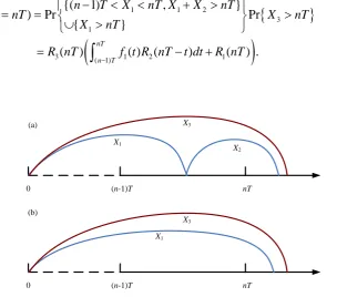
If no defective state is detected in the first (n−1) inspections, the system has to be
renewed at nT given no failure occurs before nT. This case indicates that the system
due to failure mode 1 is still in the normal state at (n−1)T and that failure in mode 2
does not occur before nT , as illustrated in Fig. 2. The corresponding occurrence
probability of this scenario is
(
)
1 1 2
3 1
3 ( 1) 1 2 1
{( 1) , }
( ) Pr Pr
{ }
( ) ( ) ( ) ( ) .
c
nT n T
n T X nT X X nT
P T nT X nT
X nT
R nT f t R nT t dt R nT −
− +
= =
=
− +(4)
0 (n-1)T nT
X1
X2
X3
0 (n-1)T nT
X1
X3
(a)
(b)
Fig.2 Renewal of the system due to the preventive replacement: (a) defective state of
failure mode 1 before nT ; (b) normal state of failure mode 1 before nT.
As previously mentioned, whenever a failure occurs, the system is renewed
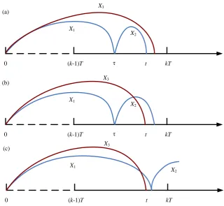
immediately. A failure occurring at t((k−1) ,T kT) implies the following two
[image:9.595.145.450.326.594.2]10
(i) The system due to failure mode 1 enters the defective state at some
((k 1) , )T t
− and leads to the system failure at t, while failure mode 2 does not
occur before t, as illustrated in Fig. 3(a);
(ii)Failure mode 2 leads to the system failure at t, and the system due to failure mode 1 is either in the normal state or the defective state at t (but is normal at (k−1)T),
as illustrated in Fig. 3(b) and Fig. 3(c).
Let Tf be the time of system failure. The PDF of Tf is given as
(
)
(
)
(
)
1 1 2 3
0
1 1 2 3
3 ( 1) 1 2
3 1 ( 1) 1 2
{( 1) , ( , ), }
1 ( ) lim Pr
{( 1) , , ( , )}
( ) ( ) ( )
( ) ( 1) ( ) ( ) ,
( 1) , , 1,..., .
f k T t t k T kT k T
k T X kT X X t t t X t f t
k T X X X t X t t t t
R t f f t d
f t R k T f F t d
t k T kT k n
→ − − − + + = − + + = − + − − − − =
(5)The probability that the system fails in ((k−1) ,T kT) is
(
)
(
)
(
(
)
)
(
)
(
(
)
)
(
) (
)
( 1)
1 3 2 3 2
( 1) ( 1)
1 3 3
3 ( 1) 1 2
1 3 3
1 3 1 3
Pr{( 1) } ( )
( ) ( ) ( ) ( ) ( ) ( 1) ( ) ( 1)
( ) ( ) ( )
( 1) ( ) ( 1) ( 1) ( 1) ( ) ( )
f
kT k
f k T T
kT t k T k T
kT k T
k T T kT f t dt
f R t f t f t F t d dt R k T F kT F k T
R kT f F kT d
R k T F kT F k T R k T R k T R kT R kT
− − − − − = = − − − + − − − = − + − − − = − − −
3 ( 1) 1 2
( ) kT ( ) ( ) . k T
R kT f R kT d −
−
−11
0 (k-1)T kT
X1
X2
τ t
X3
(a)
0 (k-1)T kT
X1
X2
τ t
(b) X3
0 (k-1)T kT
X1
X2
t
[image:11.595.139.460.78.373.2](c) X3
Fig.3 Renewal of the system due to a failure of the system. (a) Failure is due to failure
mode 1. (b) and (c): Failure is due to failure mode 2.
3.2
Expected length and cost of a renewal cycle
With the above analysis, the expected length of a renewal cycle, Tc , can be
obtained as
( 1)
1 1
1 3 3 1 2
0 ( 1) ( 1)
1
( ) ( ) ( )
( ) ( ) ( ) ( ) ( ) .
f
n n kT
k
c c k T T
k k
n
nT kT t
k T k T
k
E T kTP T kT tf t dt
R t R t dt R t f R t d dt −
= =
− −
=
= = +
= + −
(7)The term n 11 ( c )
k kTP T kT
−
= =
corresponds to the contribution of the detecteddefective state of failure mode 1, nTP T( c =nT) denotes the contribution from the
preventive replacement and
1 ( 1) f( ) kT
n k
T k= k− Ttf t dt
represents the contribution due to the12
With the corresponding probabilities derived in Section 3.1, the expected cost in a
renewal cycle can be readily obtained as
(
)
(
)
(
)
1
1
1 1
3 1 ( 1) 1 2
1
3 1 3 ( 1) 1 2
1
( ) ( ) ( ) ( 1) ( )
( 1) Pr{( 1) }
( ) ( ) ( ) ( )
( ) ( ) ( ) ( ) ( )
n
c I R c I R c
k n
I F f
k
n kT
I k T
k
n kT
R k T
k
E C kC C P T kT n C C P T nT
k C C k T T kT
C R kT R kT f t R kT t dt
C R nT R nT R kT f t R kT t dt −
=
= −
− =
− =
= + = + − + =
+ − + −
= + −
+ + −
3 1 3 ( 1) 1 2
1
1 ( ) ( ) ( ) ( ) ( ) .
n kT
F k T
k
C R nT R nT R kT f t R kT t dt −
=
+ − − −
(8)
Here,
nk−=11(kCI +C P TR) ( c =kT) represents the expected cost attributable to theinspection (the cost of k inspections) and a replacement when the defective state of
failure mode 1 is detected,
(
(n−1)CI +CR)
P T( c =nT) corresponds to the expected cost of the preventive replacement together with the expected cost of (n−1)inspections before it and
nk=1(
(k−1)CI +CF)
P k{( −1)T Tf kT} corresponds to the scenario that the system fails, including the expected cost of the inspection beforefailure and the expected cost caused by failure.
3.3
Optimal solution
Let g T n
( )
, =E T( )
c and h T n(
,)
=E C( )
c . We can have the following propertiesin terms of g T n
(
,)
and h T n( )
, .Proposition 1. g T n
(
,)
is monotonically increasing and bounded with respect to 𝑛. In addition,(
,)
0 3( )
nTg T n
R t dt13
(
)
( )
3lim ,
n→g T n E T . Therefore, when the preventive replacement is postponed, the
expected cycle length will always increase; however, the maximum will not exceed the
expectation of 𝑋3, i.e., it is bottlenecked by failure mode 2.
Proposition 2. h T n
( )
, is monotonically increasing and bounded with respect to 𝑛.(
)
( 1)( )
3 0
, I n T
F
C
h T n R t dt C
T −
+Detailed proof is shown in Appendix B. Proposition 2 implies that when the
preventive replacement is postponed, the possibility that the system is renewed by a
failure is increased, which in turn increases the cost resulting from failures. On the
contrary, the possibility that the system is renewed by a replacement is decreased, and
the expected cost of replacements is decreased. Nevertheless, the postponed preventive
replacement always increases the expected inspection cost, since it extends the expected
length of the renewal cycle. We can also have
(
)
( )
3lim , I F
n
C E X
h T n C
T
→ +
As for the inspection period 𝑇 , the corresponding derivatives of g T n
(
,)
and( )
,h T n can be obtained after tedious derivations. Forg T n
(
,)
, we have(
)
( ) ( )
( )
( )( ) (
)
(
) (
(
)
)
( )( )
(
(
)
)
1 3
3 1 1 2
1
1 1 3 2
,
1 1 1
T
kT n
k T
kT k
k T
g T n nR nT R nT
kR kT f t R kT t dt
k f k T R t R t k T dt
− =
−
=
−
+
− − − − −
14
(
)
(
)
1 3 1 1 11 3 3 1
1
, ( ) ( )
( ) ( ) ( ) ( )
n
T I n
k n
F R n
k
h T n C A kf kT R kT
C C A kf kT R kT nf nT R nT
− = − = = − + + − − +
where( )
( )( ) (
)
( )
( )( ) (
)
(
) (
(
)
)
( ) ( )
3 1 1 2 3 1 1 2
1
1 2 3
1 1
kT kT
n
k T k T
n k
kf kT f t R kT t dt kR kT f t f kT t dt A
k f k T R T R kT
− − = − + − = − − −
Then, based on ng T n
( )
, , nh T n(
,)
, Tg T n(
,)
andTh T n( )
, , the optimalinspection and replacement strategy can be readily found. Let
(
,)
(
,) ( ) (
, / ,)
f T n =ECR T n =h T n g T n , we can have
(
,)
(
, 1)
(
,)
(
(
, 1)
)
(
(
,)
)
, 1 ,
n
h T n h T n f T n f T n f T n
g T n g T n
+
= + − = −
+
(
)
(
) (
)
(
) (
)
(
)
(
)
2, , , ,
,
,
T T
T
h T n g T n g T n h T n f T n
g T n
−
=
Based on nf T n
(
,)
and Tf T n( )
, , the optimal( )
T n, that minimizes(
,)
ECR T n can be obtained straightforward. As 𝑛 is discrete, we can first find an optimal 𝑇𝑛∗ that minimizes f T n
(
,)
for fixed 𝑛, and then find the optimal 𝑛∗ thatminimizes
(
*)
,
n
f T n . Carrying on this procedure iteratively, we can find the optimal
(
* *)
,
T n .
4.
Maintenance model with imperfect inspections
In this section, we consider the effect of imperfect inspections ( 1). Denote
d
N as the number of inspections taken to detect the defective state after the occurrence
15
(
)
1(1 )i
d
P N = = −i − (Williams & Hirani, 1997). Similar as in Section 3, we
consider the following three exhaustive renewal scenarios: (1) the renewal results from
the detection of the defective state; (2) the renewal results from the preventive
replacement at the nth inspection; and (3) the renewal cycle results from a failure. (1) Consider the first scenario (where a defective state is discovered at the kth inspection,
1, 2, , 1
k = −n ). Here, the system does not fail, but rather falls into the defective state
before kT. In addition, we have Nd = − k X1/T, where x gives the maximum
integer not bigger than x. The occurrence probability of this scenario can be obtained
as
(
)
3
1 2 1 1
/ 1
3 0 1 2
3 ( 1) 1 2 1
Pr Pr , , /
( ) ( ) ( )(1 )
( ) ( ) ( )(1 ) .
c d
kT k t T
k iT
k i i T
i
P T kT X kT X X kT X kT N k X T
R kT f t R kT t dt
R kT f t R kT t dt
− − − − = = = + = − = − − = − −
(9)(2) Consider the second scenario (where the system is replaced at the nth inspection if no failure occurs and no defective state is detected before nT ). The event that no
defective state is detected consists of two scenarios: the system is in the normal state,
or the system is in the defective state but has not been discovered. Clearly, we have
1/
d
N − n X T, denoting that no defective state is detected before nT given that
the system is in the defective state. The probability of this event can be obtained as
(
)
(
)
(
)
(
)
3
1 2 1 1 1
/ 1
3 0 1 2 1
3 ( 1) 1 2 1
1
Pr
Pr , , /
( ) ( ) ( )(1 ) ( )
( ) ( ) ( )(1 ) ( ) .
c
d
nT n t T
n iT
n i i T
i
P T nT X nT
X X nT X nT N n X T X nT
R nT f t R nT t dt R nT
R nT f t R nT t dt R nT
− − − − = = = + − = − − + = − − +
(10)(3) Consider the third scenario (where either failure mode 1 or failure mode 2 leads to
system failure). The PDF that a failure occurs by time t k,( −1)T t kT is expressed
16
(
)
(
)
(
)
(
)
1 2 1 3 1
1 2 1 3
0
1 2 1 1 3
1 2 1 3
( , ), ( 1) , , 1 /
( , ), ( 1) , 1
( ) lim Pr
, ( 1) , 1 / , ( , )
, ( 1) , ( , ) f d k T t d
X X t t t X k T X t N k X T
X X t t t t X k T X t f t
t X X t X k T N k X T X t t t
X X t X k T X t t t → + + − − − + + − = + − − − + + − + =
(
)
(
)
13 ( 1) 1 2
1
3 ( 1) 1 2
1
3 ( 1) 1 2
1
3 1 ( 1) 1 2
( ) ( ) ( )(1 )
( ) ( ) ( )
( ) ( ) ( )(1 )
( ) ( 1) ( ) ( ) . k jT k j j T j t k T k jT k j j T j t k T
R t f f t d
R t f f t d
f t f R t d
f t R k T f F t d
− − − = − − − − = − − − + − + − − + − − −
(11)If is set to 1 for perfect inspection, the failure probability density of Eq. (11) is
identical to that of Eq. (5).
The renewal is resulted from either preventive replacement or corrective
replacement due to unexpected failures. After some simplifications, the expected length
of a renewal cycle is expressed as
( )
(
)
( 1)1 1
1
3 ( 1) 1 2
1 1
3 ( 1) 1 2
1 1
3 1 2
( 1) ( 1)
1
( )
( ) ( ) ( )(1 )
( ) ( ) ( )(1 )
( ) ( ) ( )(1 )
f
n n kT
k
c c k T T
k k
n k iT
k i i T k i n jT n j j T j k kT jT k j
k T j T
j
E T kTP T kT tf t dt
kTR kT f t R kT t dt
nTR nT f R nT d
tR t f R t d
− = = − − − = = − − = − − − − = = = + = − − + − − − − −
(
)
13 ( 1) 1 2
1
1 2 3
( 1) ( 1) 1
1 ( 1) 3 3 1
1
( ) ( ) ( )
( ) ( ) ( )
( 1) ( ) ( ) ( ).
n k
n kT
k T k
n kT t k T k T k
n kT
k T k
dt kTR kT f F kT d
f F t R t d dt
R k T tf t dt nTR nT R nT
= − = − − = − = + − − − + − +
(12)17
(
)
(
)
3 ( 1) 1 2
1 1
3 ( 1) 1 2 3 1
1
1
3 1 2
( 1) ( 1)
1
( ) ( ) ( ) ( )(1 )
( ) ( ) ( )(1 ) (( 1) ) ( ) ( )
( 1) ( ) ( ) ( )(1 )
n k iT
k i
c I R i T
k i
n iT
n i
I i T I R
i
k
iT jT k j
I F i T j T
j
E C kC C R kT f t R kT t dt
C R nT f t R nT t dt n C C R nT R nT
i C C R t f f t d
− − = = − − = − − − − = = + − − − − − + − + + − + − −
(
)
(
)
(
)
(
(
)
)
1 13 1 2
( 1) ( 1)
1 1
3 1 2
( 1) ( 1) 1
3 1 1 2
( 1) ( 1)
1
( 1) ( ) ( ) ( )(1 )
( 1) ( ) ( ) ( )
( 1) ( ) ( 1) ( ) ( ) .
n i
n iT k jT
k j
I F i T j T
i j
n iT t
I F i T k T
i
n iT t
I F i T k T
i
dt
i C C f t f R t d dt
i C C R t f f t d dt
i C C f t R k T f F t d dt
= − − − − = = − − = − − = + − + − − + − + − + − + − − −
(13)With the expression of E T( )c and E C( c), we can derive the ELRCR according to
Eq. (2). Then, with the given T and n, one can easily calculate the corresponding
long-run cost rate. The optimal (T n, ) that minimizes the ELRCR can be easily
derived with numerical methods. The current model can be extended to the cases with
arbitrary preventive replacement interval and with time-dependent inspection
probability. We present these extensions in Appendix C and Appendix D for
compactness of the paper.
5.
Case Study
Infusion pumps are important equipment to pump fluids for patients. Infusion
pumps contain a variety of types, among which the widely used type is the peristaltic
pump. A peristaltic pump usually suffers two failure modes. One is due to the battery
which is routinely checked up of its voltage, the other is the electrical parts failure which
cannot be monitored. The battery goes through a degradation process before failure,
which can be described with a delay-time failure model, while the electrical parts are
18
and X2 to denote the duration of the normal state and the deterioration state of the
battery and X3 to denote the lifetime of the electrical parts. The three variables are
assumed to follow Weibull distributions ( ) 1 exp
(
/)
i
i i
F x = − − x , where the
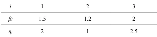
distribution parameters are as given in Table 1. The inspection cost, replacement cost
[image:18.595.140.454.252.326.2]and failure cost are set as CI =10, CR =100and CF =800, respectively.
Table 1 Distribution parameters for lifetime distributions of the peristaltic infusion pump.
i 1 2 3
βi 1.5 1.2 2
ηi 2 1 2.5
5.1
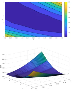
Illustration of the model proposed in Section 3
With the given parameter setting, the optimal inspection interval and preventive
replacement interval are obtained as (T n, )=(0.23,6). This indicates that the optimal
inspection interval is 0.23 and that preventive replacement should be carried out at the
sixth inspection if no failure occurs before it. The expected cycle length and the
expected cycle cost are E T( )c =0.6165 and E C( c)=98.28 , respectively, while the
optimal ELRCR is ECR T n( , )=152.2. Fig.4 shows how the ELRCR varies in terms
19
Fig.4 Variation of ELRCR in terms of n and T
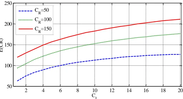
To show the influence of the cost parameters on the optimal inspection and maintenance
strategy, Fig. gives the variation of the optimal (T n, ) and ECR T n( , ) for
different inspection cost CI and replacement cost CR. It is shown that the optimal inspection interval T increases monotonically with CI , indicating that the
inspection tends to be less frequent as the unit inspection cost increases. In addition, the
optimal inspection interval T decreases with the replacement cost CR. Actually, the
cost for inspection is relatively cheaper when the cost for replacement increases, thus it
20
inspection interval) can attenuate the risk of system failure and thus reduce the
maintenance cost, which is more effective for the system with a higher replacement
cost. In contrast, as the inspection becomes less frequent, n decreases to ensure that
the risk of failure due to failure mode 1 can be controlled under a certain level. With an
increased inspection interval, the number of inspections should be decreased so as to
balance the probability of failure. This logic is illustrated in the middle panel of Fig.,
where the optimal preventive replacement interval n decreases with the inspection
cost CI and decreases with the replacement cost CR . Clearly, ELRCR always
increases with CI and CR.
2 4 6 8 10 12 14 16 18 20
0 0.1 0.2 0.3 0.4 0.5 0.6 0.7
C
I
T
*
C
R=50
CR=100
CR=150
2 4 6 8 10 12 14 16 18 20
0 5 10 15 20
C
I
n
*
C
R=50
C
R=100
C
21
Fig.5 Variation of the optimal (T n, ) and the optimal ELRCR with respect to the
inspection cost CI for different CR.
5.2
Illustration of the model proposed in Section 4
Consider the case with imperfect inspections. The probability of detection is set as
0.7
= . In this setting, the optimal inspection interval T and the optimal preventive
replacement cycle n are obtained as (T n, )=(0.27,5) . The associated expected
cost in a renewal cycle E C( c) and length of a cycle length E T( )c are obtained as
( c) 118.7
E C = and E T( )c =0.7431, respectively. The optimal ELRCR is achieved as
( , ) 159.8
ECR T n = . Fig.6 presents how the ELRCR varies with different n and T.
2 4 6 8 10 12 14 16 18 20
50 100 150 200 250
CI
E
(CR)
C
R=50
CR=100 C
22
Fig.6 Variation of ELRCR with respect to n and T
Compared with the scenario of perfect inspection in Section 5.1, the existence of
imperfect inspection leads to a larger ELRCR. This is because the failed detection of
the defective state increases both the renewal cycle length and the maintenance cost in
a renewal cycle. In contrast, the preventive replacement interval n is smaller, as the
imperfect inspection increases the risk of failure; thus, the system should be
preventively replaced more frequently. In addition, we plot the variations of (T n, )
and the corresponding ECR T n( , ) with respect to different inspection cost CI and
replacement cost CR, as shown in Fig.. It is obvious that ECR T n( , ) increases with
the inspection cost CI and replacement cost CR. However, the monotonic trend of
the optimal preventive replacement interval n and optimal inspection interval T is
not as apparent as that for the basic model of Section 3. It can be seen that n decreases
23
Fig.7 Variation of the optimal (T n, ) and the optimal ELRCR with respect to CI
and CR for imperfect inspection.
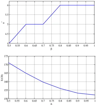
To investigate the effect of on the optimal maintenance policy, we plot the
2 4 6 8 10 12 14 16 18 20
0 0.1 0.2 0.3 0.4 0.5 0.6 0.7
C
I
T
*
CR=50
C
R=100
CR=150
2 4 6 8 10 12 14 16 18 20
0 5 10 15 20
C
I
n
*
CR=50
CR=100
CR=150
2 4 6 8 10 12 14 16 18 20
50 100 150 200 250
CI
E
(C
R
)
C
R=50
C
R=100
C
24
variation of the optimal (T n, ) and the corresponding ECR T n( , ) with the
detection probability , as shown in Fig.. From Fig., we can see that ECR T n( , )
decreases monotonically with respect to , which indicates that an improved detection
accuracy contributes to the reduction of maintenance cost. The optimal inspection T
shows a non-increasing trend with , while the optimal preventive replacement cycle
n shows a non-decreasing trend with . This is because, when the detection
probability is small, inspection should be carried out less frequently as the effect of
inspection is not significant. Instead, more effort should be placed on the preventive
replacement, and a more frequent preventive replacement is advocated. The sensitivity
analysis on implies that companies should pay more effort into improving the
detection accuracy, so as to reduce the maintenance cost.
0.5 0.55 0.6 0.65 0.7 0.75 0.8 0.85 0.9 0.95 1 0.22
0.24 0.26 0.28 0.3 0.32
T
25
Fig.8 Variation of the optimal (T n, ) and the optimal ELRCR with respect to the detection probability.
5.3
Comparison with block replacement and age-based maintenance
To show the effectiveness of the proposed maintenance policy, we compare the
proposed maintenance policy with two traditional maintenance policies: block
replacement and age-based maintenance policy. Block replacement policy implies that
the system is replaced at failure, while no preventive replacement and inspection is
implemented to prevent unexpected failures. With the block replacement policy, the
expected length of a renewal cycle is 1.727 and the ELRCR is obtained as
463.22
ECR= .
Age-based maintenance indicates that the system is replaced either at failure or at
0.5 0.55 0.6 0.65 0.7 0.75 0.8 0.85 0.9 0.95 1 4
4.5 5 5.5 6
n
*
0.5 0.55 0.6 0.65 0.7 0.75 0.8 0.85 0.9 0.95 1 150
155 160 165 170 175
E
(C
R
26
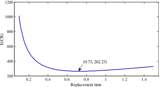
a specific age. Fig. 7 shows how the ELRCR varies with different replacement age. It
can be observed that the optimal age-based maintenance policy is achieved when the
replacement age is 0.73. The expected length of a renewal cycle and the expected cost
in a renewal cycle are given as 0.7014 and 183.94, respectively. The optimal ELRCR
is obtained as *
262.23
ECR = . Compared with these two maintenance policies, it can
be concluded that the proposed maintenance policy is more effective in reducing the
maintenance cost. In addition, the results imply the importance of inspection for a
[image:26.595.152.463.274.440.2]system with the delay-time failure mode.
Fig.4 ELRCR for an age-based maintenance policy.
6.
Summary and final remarks
This paper considered a single-unit system subject to two failure modes, where one
failure mode can be modeled by a two-stage delay-time model and the other by a
traditional hard failure. For practical systems that consist of multiple failure modes,
these failure modes with delay-time could be aggregated as one mode, whilst those
failure modes that do not have any detectable defective states before failure could be
aggregated as the other mode. Periodic inspections were conducted to detect the
possible defective state of the system, and preventive replacements were implemented
to mitigate the failure caused by the catastrophic failure mode. We formulated this
0.2 0.4 0.6 0.8 1 1.2 1.4
200 400 600 800 1000 1200
Replacement time
E
(CR)
27
maintenance model and studied the impact of the inspection interval and preventive
replacement time on the system performance. Our initial model was then further
extended to account for imperfect inspections. The optimal maintenance strategy was
investigated and illustrated through a case study of peristaltic infusion pump.
As a direction for future study, the two-stage failure process in this paper can be
extended to a three-stage failure process to enable more accurate modeling.
Additionally, since the real-world applications generally do not function over an infinite
time horizon, the model could be adapted to a finite interval. The dependence between
the two failure modes could also be considered in the future. Moreover, failure-inducing
inspection is another potential extension, which can be used for multi-component
systems.
Acknowledgements
The research is supported by the NSFC under grant number 71671016 and
71231001, and by the Fundamental Research Funds for the Central Universities of
China FRF-BR-15-001B.
Appendix A:
Proof of Proposition 1
It is straightforward to have the derivative of g T n
(
,)
with respect to n as(
)
(
) (
)
( ) ( )
(
( ) (
)
)
( 1)
3 1 1 2
, , 1 ,
0
n
n T t
nT nT
g T n g T n g T n
R t R t f R t d dt
+
= + −
=
+
− 28
(
)
( ) ( )
( )
( ) ( )( ) (
)
( ) ( )
( )
( )(
(
(
)
)
( )
)
(
)
(
)
( )( )
( )
1 3 03 1 2
1 1
1
1 3 0
3 1 1
1 1
1 1 3 0 3
1
,
1
1
nT
n kT t
k T k T
k nT
n kT
k T k
n kT nT
k T k
g T n R t R t dt
R t f R t d dt
R t R t dt
R t R k T R t dt
R k T R t dt R t dt
− − = − = − = = + − + − − = −
Appendix B:
Proof of Proposition 2
The derivative of h T n
( )
, with respect to n can be obtained as(
)
(
) (
)
( ) ( )
(
( )( ) (
)
)
(
)
( ) ( )
(
(
)
)
(
(
)
)
(
)
(
)
( )( )
(
(
)
)
3 1 1 1 2
1 3 1 3
1
3 1 2
, , 1 ,
1 1
0
1 1
n
nT
I n T
n T
F R
nT
h T n h T n h T n
C R nT R nT f t R nT t dt
R nT R nT R n T R n T
C C
R n T f t R n T t dt
− + = + − = + − − + + + − − + + −
Meanwhile, we have
(
)
( ) ( )
(
( )( ) (
)
)
( ) ( )
( )
( )( ) (
)
( ) ( )
( )
( )( ) (
)
( ) (
(
)
)
( )( )
1
3 1 1 1 2
1
1 3 3 1 2
1 1
1 3 3 1 1 2
1
1 1
3 1 3
0 1 , 1 1 n kT
I k T
k n kT R k T k n kT
F k T
k
n n T
I
I F F
k
h T n C R kT R kT f t R kT t dt
C R nT R nT R kT f t R kT t dt
C R nT R nT R kT f t R kT t dt C
C R kT R k T C R t dt C
T − − = − = − = − − = = + − + + − + − − − − + +
Appendix C:
Maintenance model with
arbitrary preventive replacement
interval
29
As the system has to be replaced by time TR, the maximum number of inspections is
/
R
T T
. A renewal cycle ends with either preventive replacement or corrective
replacement, and we now consider all the possible scenarios this entails.
(1) A defective state is discovered at the kth inspection (k =1, 2, ,Tr /T). In this
case, we have Nd = − k X1/T. The occurrence probability of this scenario can be
readily obtained by Eq. (9), with the constraint that kis limited as k=1, 2, ,Tr /T.
(2) The system is replaced by time TR if no failure occurs and no defective state is
detected before TR. If the system is in the defective state but has not been identified by
inspections, we have Nd TR/T − X1/T . The probability of preventive
replacement at time TR can be obtained as
(
)
(
)
(
)
(
)
3
1 2 1 1 1
/ /
3 0 1 2 1
Pr
Pr , , / /
( ) R ( ) ( )(1 ) R ( ) .
c R R
R R d r R
T T T t T
R R R
P T T X T
X X T X T N T T X T X T
R T f t R T t − dt R T
= =
+ −
=
− − +(3) A failure occurs if no defective state is discovered and no preventive replacement is
30
/
/ 1
3 ( 1) 1 2
1
3 / 1 2
/
/ 1
3 ( 1) 1 2
1
3 / 1 2
3 1
( ) ( ) ( ) ( )(1 )
( ) ( ) ( )
( ) ( ) ( )(1 )
( ) ( ) ( ) ( ) ( )
f
t T
jT t T j
T j T
j t
t T T t T
jT t T j
j T j
t t T T
f t R t f f t d
R t f f t d
f t f R t d
f t f R t d
f t R t
− + − = − + − = = − − + − + − − + − +
/ /3 0 1 2
/ /
3 0 1 2
3 1
= ( ) ( ) ( )(1 ) ( ) ( ) ( )(1 ) ( ) ( ).
t t T T
t t T T
R t f f t d
f t f R t d
f t R t
− − − − + − − +
Accordingly, the expected length of a renewal cycle is
( )
(
)
(
)
(
)
/ 0 1 / / 13 0 1 2
1
/ /
3 0 1 2 1
/
3 0 1 2
( )
( ) ( ) ( )(1 )
( ) ( ) ( )(1 ) ( )
( ) ( ) ( )(1 ) R R f R R R T T T
c c R c R T
k T T
kT k t T
k
T T T t T
R R R R
t t T
E T kTP T kT T P T T tf t dt
kTR kT f t R kT t dt
T R T f t R T t dt R T
R t f f t t = − − = − − = = + = + = − − + − − + − − +
/ / /3 1 2
0 0
3 1
( ) ( ) ( )(1 ) . ( ) ( )
R
T
T t t T T
d
f t f R t d dt
f t R t
− + − − +
The expected cost in a renewal cycle is
(
)
(
)
(
)
(
)
/
/ 1
3 0 1 2
1
/ /
3 0 1 2 1
/ /
3 0 1 2
3 1
( ) ( ) ( ) ( )(1 )
/ ( ) ( ) ( )(1 ) ( )
( ) ( ) ( )(1 )
+ / ( )
R
R
R
T T
kT k t T
C I R
k
T T T t T
R I R r R R
t t T T
I F
E C kC C R kT f t R kT t dt
T T C C R T f t R T t dt R T
R t f f t d
t T C C f t f
− − = − − = + − − + + − − + − − + +
/ / 2 0 0 3 1( ) ( )(1 ) .
( ) ( )
R
T t t T T
R t d dt
f t R t
31
Appendix D:
Maintenance model with t
ime dependent detection
probability
If the inspection accuracy is dependent on the time from the initial point of defective
stage to the time of inspection, denoted as ( )t , we can obtain the maintenance cost
and length in a similar way as in Section 4. The probabilities of the renewal from
inspections and failures are expressed in the following equations.
(
)
3 0 1 2 / 11
( ) ( ) ( ) (1 ( / )) ( )
k t T kT
c
j
P T kT R kT f t R kT t jT t T T t kT t dt − −
=
= =
−
− + − − ,(
)
3 0 1 2 / 1 11
( ) ( ) ( ) (1 ( / )) ( )
n t T nT
c
j
P T nT R nT f t R nT t jT t T T t dt R nT − − = = = − − + − +
, 1 / 13 ( 1) 1 2
1 1
3 ( 1) 1 2
1 / 1
3 ( 1) 1 2
1 1
( ) ( ) ( ) ( ) (1 ( / ))
( ) ( ) ( )
( ) ( ) ( ) (1 ( / ))
f
k T
k iT k
T i T
i j t k T k T k iT i T i j
f t R t f f t jT T T d
R t f f t d
f t f R t jT t T T t d
− − − − = = − − − − − = = = − − + − + − + − − + −
(
)
(
)
3 1 ( 1) 1 2
( ) ( 1) t ( ) ( ) k T
f t R k T f F t d −
+ − −
−.
Based on the above equations, the expected length and cost of a renewal cycle can be
readily obtained.
References
Aven, T., Castro, I.T., 2009. A delay-time model with safety constraint. Reliability Engineering & System Safety, 94(2), 261-267.
Berrade, M.D., Cavalcante, C.A.V., Scarf, P.A., 2012. Maintenance scheduling of a protection system subject to imperfect inspection and replacement. European Journal of Operational Research, 218(3), 716-725.
Berrade, M.D., Cavalcante, C.A.V., Scarf, P.A., 2013. Modelling imperfect inspection over a finite horizon. Reliability Engineering & System Safety, 111,18-29.