Abstract No. F180130-142
Object Detection Algorithm for Unmanned Surface Vehicle using
Faster R-CNN
Author name(s): Heesu Kim1 Evangelos Boulougouris2 Sang-Hyun Kim3
1. Department of Naval Architecture, Ocean and Marine Engineering, University of Strathclyde, UK 2. Department of Naval Architecture, Ocean and Marine Engineering, University of Strathclyde, UK 3. Department of Naval Architecture and Ocean Engineering, Inha University, South Korea
The purpose of this research is development of vision-based object detection algorithm that recognizes a marine object, localizes the object on captured frames, and estimates the distance to the object. Faster R-CNN and stereo vision based depth estimation are combined for real-time marine object detection. The performance of this algorithm is verified by model ship detection test in towing tank. The test results showed that this algorithm is potentially applicable to real USV.
KEY WORDS: Unmanned surface vehicle; vision-based object detection; faster region with convolutional neural network; depth estimation.
NOMENCLATURE
AIS, automatic identification system CNN, convolutional neural network
Faster R-CNN, faster region with convolutional neural network GPU, graphics processing unit
ILSVRC, ImageNet large scale visual recognition competition IoU, intersection over union
LiDAR, light detection and ranging LRF, laser rangefinder
mAP, mean average precision
PASCAL VOC, PASCAL visual object classes Radar, radio detection and ranging
ReLU, rectified linear unit RPN, region proposal network; USV, unmanned surface vehicle INTRODUCTION
The autonomous system is becoming an essential part of our life, reducing human labor and human error. The automatic system has found its way into the various control system such as processes in factories, switching on telephone networks, heat treating, etc. Over time, the automatic system technology has been advanced and the concepts of the fully automatic system, called automation, have been arising. This system is usually accomplished in combination with complex systems, such as modern factories, airplanes, and ships.
Accordingly, there is rapid growth in unmanned vehicle development such as unmanned ground and aerial vehicle for supporting transportation, surveillance environment investigation and so on. In the marine industry, there has been an effort on development of USV. It operates on the sea surface without crew and is becoming popular due to its reduced cost compared to for example research and oceanographic ships, and being more efficient than weather buoys. They are commonly designed to accomplish their mission from the commands transmitted remotely without humans’ instant control or programmed to perform regularized actions repeatedly. This
helps avoiding marine accidents mostly caused by human error (Campbell, Naeem, and Irwin 2012).
As vessels are automated, the significance of obtaining and processing the data surrounding the operating vehicles for safe navigation has increased. The collision avoidance through proper path planning ensures also prevention from a crash accident. Accordingly, it requires decent sensor system that detects accurately and processes the obtained data to applicable information that can be used for pertinent action.
In order to collect such data, the majority of USV is equipped by various sensors such as sonar sensor, AIS, LiDAR, Radar and vision sensor for detecting obstacles or other vessels. However, most of this equipment has disadvantages as they are expensive or difficult to install on a small ship due to their massive weight. This necessitates the simplification of the equipment and the reduction of their number. In this regard, the use of a vision sensor is powerful for USV where near obstacles are closely related to collision risk, in place of other expensive and heavy detection equipment. Furthermore, it can enhance detection by supporting existing detection system in large vessels.
Due to use of the vision sensor, it is required to process an image to recognize objects. In order for a USV to recognize an object without human intervention, it is important to possess object recognition ability comparable to that of a human being. For this purpose, this research uses the CNN which specializes in image processing more than other machine learning techniques. The CNN is a state-of-art technique of computer algorithms, mimicking animal’s visual perception and learning abilities. Intelligent animals and humans obtain the ability of object recognition by learning the images and their corresponding names by experience over a long period of time. As the CNN works similarly, it requires a large number of images, many computational iterations, high computational power and time. Recently, due to the remarkable developments in data science, it is not difficult to collect a large number of datasets. Moreover, improvement of computer capacity reduced computation time significantly.
users (Woo 2016; Woo and Kim 2016; Wang and Wei 2013; Wang, Wei, Wang, Ow, Ho, Feng, et al. 2011; Wang, Wei, Wang, Ow, Ho, and Feng 2011; Sinisterra, Dhanak, and von Ellenrieder 2014; Gladstone et al. 2016; Shin et al. 2018). Although it can be called automation, there is still a human error because it is eventually set by a human. The CNN can mitigate this problem by extracting the features on its own reducing human intervention. In this context, this research was motivated to apply the vision sensor, one of the economical and lightweight equipment to automatic navigation.
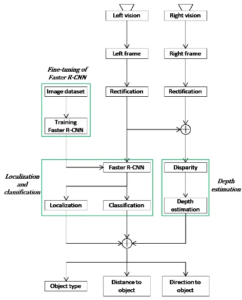
The aim of this research is to implement an algorithm to recognize other objects or ships using a stereo camera for autonomous navigation of USV. Faster R-CNN (Ren et al. 2015) is used for real-time classification and localization based on CNN, and depth estimation method is used to estimate the distance to detected objects. As a preliminary process, the CNN and RPN in the Faster R-CNN are fine-tuned. When the algorithm starts to run, a left frame passes through the whole network of the Faster R-CNN, and it classifies and localizes the observed objects. After this, from the left and right vision, the 3D point cloud is created all over the pixels. By matching the local information and the 3D point cloud obtained from the Faster R-CNN and depth estimation, it estimates the distance to the objects. This process is repeated in real-time.
ALGORITHM ARCHITECTURE
The project is composed by two stages as shown in Fig. 4. The first stage is localization and classification performed by Faster R-CNN. In this stage, the process is carried out with only left frame acquired from left view. It provides the information of object type and the location on the frame. The second stage is depth estimation. It utilizes both side frames and figures out the depth, which represents the distance to an every pixel point. This process furnishes the information of distance to object mobilizing object local data obtained from the Faster R-CNN.
Modification of Faster R-CNN
Although there is a default configuration in Faster R-CNN that gives the best performance in VOC2017 (Everingham et al. 2007), some configurations are modified to be suitable to recognize the ship as it has not been utilized in the marine industry.
CNN Model
[image:2.612.328.564.55.348.2]There are many CNN models that have been released such as ALexNet (Krizhevsky, Sutskever, and Hinton 2012), ZF Net (Zeiler and Fergus 2014), VGG Net (Simonyan and Zisserman 2014), GoogLeNet (Szegedy et al. 2015), Microsoft ResNet (He et al. 2016), etc. As such these networks are becoming deeper and deeper, they showed higher accuracy in classification. However, although they are improved, they also require higher GPU memory capacity as it processes more massive data. It restricted the options for using the best network among them. Due to this reason, we selected ZF Net that does not cause out of the memory of GPU that used in this research.
Fig. 4. Project architecture
ZF Net is the network that won the ILSVRC 2013. This model reached an 11.2% error rate and was fine-tuned more than the AlexNet architecture, which won the ILSVRC 2012. It is alike to AlexNet, but with a few slight alterations, it has improved performance. ZF net uses 7 × 7 filters instead of 11 × 11 filters used in AlexNet, and the stride is also reduced. This allows the first convolutional layer to maintain a lot of initial pixel information. ReLU is used for the activation function, the cross-entropy loss is used for error function, and batch stochastic gradient descent is used for training (Deshpande 2016).
Anchor
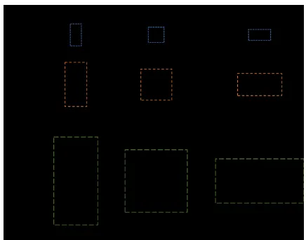
In the Faster R-CNN process, the input image is scaled such that their shorter side becomes 600 pixels while the long side does not exceed 1000 pixels before it is fed into a network. Therefore, the 640 × 480 pixels image captured by the stereo camera is scaled to 800 × 600 pixel. The anchors propose regions on this scaled image with its size of 1282 pixels, 2562 pixels, 5122 pixels and its ratios of 1:2, 1:1 and 2:1 as shown in
Fig. 6. Scaled image and applied anchors
Fig. 7. Default anchors
In this process, there is a critical drawback to detect a small object. For example, if it detects a side of a small ship that is
3 m long and 50 m away, the ship occupies around 30 × 6
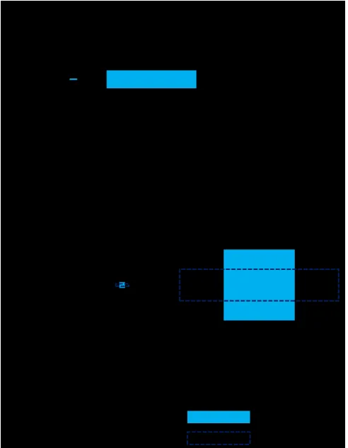
[image:3.612.54.272.163.334.2]pixels on the captured image, and it is scaled to 37 × 7 pixels. At the moment the smallest anchor slides over the object region, as shown in Fig. 8, the IoU is only 0.016, which is much smaller than default IoU threshold 0.7 to be considered as positive. With this default anchor, the ground-truth box smaller than 902 pixels cannot be labelled as positive.
Fig. 8. The overlap between 1282 anchor and small object
Therefore, the anchor size and ratio are recommended to be set to at least 162 pixels and 5:1, as shown in Fig. 9, respectively, to maximize the IoU.
Fig. 9. Size comparison between 162anchors with the ratio of
5:1
Accordingly, we modified the anchor configuration from the default of it, to fit to detect a ship-shaped object in distance.
A 2 m-long small ship occupies 350 × 70 pixels at a distance of
4 m, and 30 × 6 pixels at a distance of 50 m, on the captured image from the stereo camera. These sizes are scaled to 438 × 88 pixels and 37 × 7 pixels, respectively. Correspondingly, the optimal range of anchor size is from 162 pixel to 1962 pixel with the ratio of 5:1. Because changing the size and ratio of anchor from its default reduces its mAP (Ren et al. 2015), we followed the anchor size and IoU threshold from Faster R-CNN for small logo detection (Eggert et al. 2017), to minimise the loss of mAP, and also modified the setting to drop small boxes as changing minimum box size from 162 to 22 to enable to detect small area. The anchor configuration is shown in Table 1.
Table 1. Default and modified anchor configurations
Anchor
configuration Default Modified
Anchor size (pixels) 128
2, 2562, 5122 82, 162, 322, 442,
642, 902, 1282, 2562 Anchor ratio 2:1, 1:1, 1:2 4:1, 5:1, 6:1
IoU threshold 0.7 0.5
Minimum box size (pixels)
162 22
Dataset
The powerful advantage of CNN is that it can classify objects by generalizing same labelled objects into one category, although they have various appearances. It can be proved clearly if the experiment is carried out on real sea observing various real ships. However, in this research, the actual sea area test was replaced with an experiment that detects the model ship in the towing tank because there are many practical limitations such as preparing and measuring real distance. Therefore, the dataset consists of only one class of model ship.
A notable point in this section is the size of an object in an image used for training. As the anchor sizes are reduced overall from default, proposals that are assigned as positive during training are required to be considered carefully. For example, assume that there is a 600 × 400 pixels object in an 800 × 600
[image:3.612.53.285.464.539.2]Fig. 10. Anchors labelled positive and negative on a large object and small object
Therefore, in order to detect small objects, anchors must capture the outline of the object as a feature. This means that the scaled object size of the dataset image should be similar to the scaled size of the object to be detected.
As the model ship is observed between the distances from 4 m
to 50 m during the experiment, the ground-truth box of model ship occupies pixels from 37 × 7 pixels to 438 × 88 pixels, in
800 × 600 pixels scaled image. Accordingly, ground-truth box size in image datasets to be prepared are recommended to occupy pixels from 37 × 7 pixels to 438 × 88 pixels, where the area ratios of scaled images to the ground-truth boxes are
1: (5.40 × 10⁻⁴) and 1: (8.03 × 10⁻²) , respectively. For example, if there is a 1500 × 1000 pixels image in a dataset, the ground-truth box area is required to occupy the pixels from
(1500 × 1000) × (5.40 × 10−4) to (1500 × 1000) ×
[image:4.612.32.297.47.255.2](8.03 × 10−2), e.g., from 810 pixels to 120450 pixels as shown in Fig. 11. Additionally, as the aspect ratio of the ground-truth box in dataset image closes to the anchor ratio, there is a high probability that anchors sliding over the object labelled as positive.
Fig. 11. Example of recommended ground-truth box in dataset
image
The image dataset of the model ship to be used for the training was prepared by taking a picture of it. If the size of the object on the taken images is large, a margin is added to the edge of the images to satisfy above conditions. The number of dataset images is around 1000, referring to the PASCAL VOC 2007 dataset (Everingham et al. 2007).
Depth Estimation
The distance to object is important information for collision risk assessment. This section describes the process to calculate the distance to object. Unlike the case where only the left frame is used in Faster R-CNN, both frames are used in depth estimation and it calculates the distance to object based on the location of the object obtained from the Faster R-CNN.
Fig. 12. Workflow of depth estimation
Distance to Object
The Faster R-CNN represents the position of the object as a final output giving bounding boxes accompanying the values of left bottom point and right top point. From these values, we extracted the center point of the bounding box as following Eq. 3.
(𝑥𝑐, 𝑦𝑐) = (
𝑥1+ 𝑥2
2 ,
𝑦1+ 𝑦2
2 ) (3)
where (xc, yc) is the centre point of bounding box, (x1, y1) and
(x2, y2) are the left bottom point and right top point of bounding box respectively. By matching this value to 3D point cloud map, the hypothetical distance to object, zo, is calculated. This process is shown in Fig. 13.
Fig. 13. Workflow of distance estimation
DETECTION TEST
Stereo Camera
The specification of the stereo camera used in this research is described in Fig. 14 and Table 2. In this research, resolution and frame were set to 640 × 480 MJPEG and 30fps respectively due to memory limitation during computation.
Computer Capacity
The computer environment in which the computation is performed is indicated in Tables 3.
Detection Test Environment
The detection test was carried out by observing the model ship in a towing tank. The geometry is shown in Fig. 15. Since the LRF outputs the voltage according to the distance to the board, we measured the voltage and actual distance at three points and calibrated it.
The length of the model ship used in the experiment is shown in
[image:5.612.72.256.47.257.2]Fig. 14. Stereo camera
Table 2. Stereo camera specification
Model name KYT-U100-960R1ND Sensor Aptina AR0130
Focus Manual
Synchronization Yes
Resolution & frame 640 × 480 MJPEG 30fps, YUY2 15fps
1280 × 960 MJPEG 30fps, YUY2
5fps Compression
format MJPEG \ YUY2
Interface USB2.0
Lens Parameter Non Distortion Lens, FOV 96°(D), 80°(H), 60°(V)
Voltage DC5V
UVC Support
OTG Support
Auto exposure AEC Support Auto white balance
AEB
Support Adjustable
parameters Brightness/Contrast/Color saturation/Definition/Gamma/WB Dimension 74mm x 27mm
Operating
Temperature -20°C to 70°C
Support OS Windows, Linux, MAC, Android
Table 3. Computer environment
Computer Components Specification CPU Processor Intel Core i7 6700 CPU @
3.40GHz
Cores 4
Threads 8
Mainboard Model W650DC
Chipset Intel Skylake Southbridge Intel H170
Memory Type DDR 4
Size 8 Gbytes Graphics
Card
Memory Type GDDR 5 Memory Size 4096 MB
Matlab Version R2016b
Fig. 15. Towing tank geometry during detection test
Fig. 16. The model ship used in detection test
Dataset
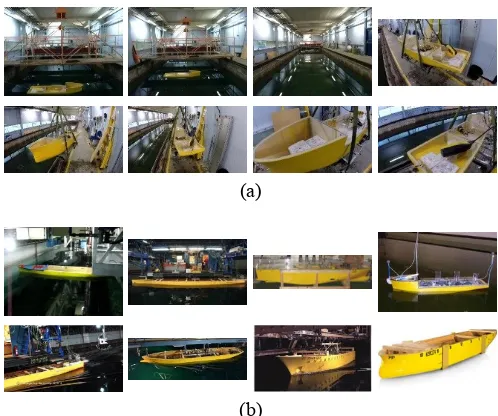
In order to observe the performance of the algorithm proposed in this research, the detection test were carried out by changing dataset image, which has a large effect on the CNN performance. As the dataset, images of the model ship used in this detection experiment and of the other model ships have prepared as shown in Fig. 17.
(a)
[image:6.612.36.292.163.496.2](b)
Fig. 17. Image samples in the dataset. (a) Image of model ship
used in the detection system. (b) Image of the model ship not used in detection test
Network Configuration
[image:6.612.323.572.418.626.2]observe the performance of the algorithm according to the dataset type and proposal configuration as described in Table 4.
Table 4. Dataset type and proposal configuration of networks for
detection test Network
case
Dataset type
Same model ship
Different model ship
Total amount
Case 1 930 104 1034
Case 2 930 104 1034
Case 3 0 303 303
Case 4 241 0 241
Network
case Proposal configuration
Anchor size Anchor ratio
IoU threshold Case 1 1282, 2562, 5122 1:2, 1:1, 2:1 0.7 Case 2 42, 82, 162, 322,
442, 642 , 902,
1282, 2562
1:4, 1:5, 1:6 0.5
Case 3 42, 82, 162, 322,
442, 642 , 902,
1282, 2562
1:4, 1:5, 1:6 0.5
Case 4 42, 82, 162, 322,
442, 642 , 902,
1282, 2562
1:4, 1:5, 1:6 0.5
The network for case 1 is set to default proposal configuration and trained with the same model ship dataset image that will be observed in the test. This is for taking a see how powerful the existing CNN is with default configuration and for comparison with other modified networks. In case 2, the dataset is same to case 1 but the proposal configuration is changed. This configuration is modified for the purpose of small object detection. In case 3, the proposal configuration is same to case 2 but the dataset is composed by other model ship that is different from what will be observed. This is to see how much the network recognizes when it is trained with a limited dataset. Case 4 is to see the effect of the amount of dataset. It has relatively small amount of dataset. In order to calculate mAP, the dataset consists of the 70% of train images and the 30% test images.
Test Result
Network Training Result
The results of training each network are shown in Table 5. The mAP is a factor that evaluates the quality of dataset and is an index of how much the test set relates to the train set. The higher the value, the higher the associativity between images of the
datasets. Since the mAP of the ZF net trained with the PASCAL VOC 2007 dataset is 59.9% (Ren et al. 2015), the dataset used in this research is judged to be collected appropriately.
Table 5. Training and detection results of networks for each case
Network case Train-Time
(hour) mAP (%)
Case 1 18.57 66.04
Case 2 19.75 72.58
Case 3 18.27 79.87
Case 4 18.83 63.27
Detection Test Result
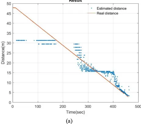
In the first detection test, the detection algorithm ran while the carriage with the stereo camera approaches to the model ship. It was carried out for each network in four cases. The initial distance between the stereo camera and the model ship is
47.86 m, and the speed of the carriage is 0.1 m/s. It starts moving after 10 sec from the start of the camera recording. The results of detection test are shown in Fig. 18. In all cases, the mean computing time per frame was 0.33 sec so that it is considered that there is no problem in real-time detection.
[image:7.612.335.566.320.524.2](b)
(c)
[image:8.612.48.279.48.680.2](d)
Fig. 18. . The result of detection and distance estimation (a)
network case 1. (b) network case 2. (c) network case 3. (d) network case 4.
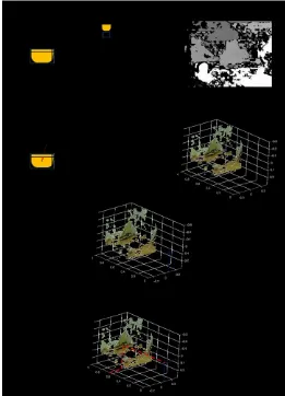
However, it was not able to estimate the distance more than
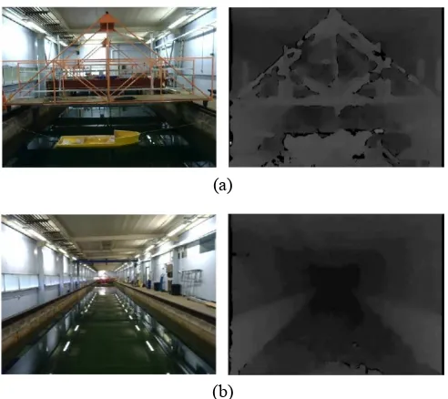
[image:8.612.326.572.240.459.2]31.3 m. The reason is due to the depth estimation technique, which is built on disparity images. Since the disparity images are drawn based on the texture of the image, wrong disparities can be included due to low texture, low pixel, etc. (Hirschmuller 2005). As the distance increases then the pixel containing visual information reduces, inaccurate disparities are generated and the accuracy of the distance estimation decreases. The example of disparity images at the distance of 47 m and 3 m is shown in
Fig. 19. The plateau between 300 and 400 sec in the cases 1, 2 and 4 (Fig. 18 (a), (b) and (c)) are also explained for the same reason.
(a)
(b)
Fig. 19. Disparity image. (a) Original frame and disparity image
at the distance of 3 m. (b) Original frame and disparity image at the distance of 47 m
Except for the detection farther than 31.3 m, cases 1, 2, and 4 generally estimated distances close to the actual distance. However, in case 3, only the distance within 5 m was estimated appropriately, and in case 4, excessive wrong detection occurred.
The percentages of the well-detected frame, calculated as in Eq. 4, and mean distance errors excluding the distance of more than
𝑇ℎ𝑒 𝑛𝑢𝑚𝑏𝑒𝑟 𝑜𝑓 𝑤𝑒𝑙𝑙 − 𝑑𝑒𝑡𝑒𝑐𝑡𝑒𝑑 𝑓𝑟𝑎𝑚𝑒𝑠
𝑇𝑜𝑡𝑎𝑙 𝑛𝑢𝑚𝑏𝑒𝑟 𝑜𝑓 𝑓𝑟𝑎𝑚𝑒𝑠 × 100 (%) (4)
Result comparison between case 1 and case 2; focusing on proposal configuration
In cases 1 and 2, the dataset image is the same as the model ship used in detection test, and the number of those was large enough. The difference between the two cases was the proposal configuration, where case 2 has more anchor sizes than case 1 and the anchor ratio is closer to the size of the model ship used in this test. The IoU threshold of case 2 was also set to a smaller than case 1.
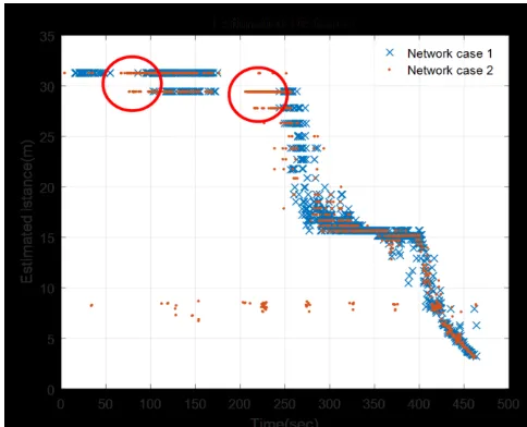
The percentage of well-detected frame in case 1 and case 2 was 59.77% and 65.85%, respectively. This shows that the modified proposal configuration improved the recognition success rate by
[image:9.612.330.572.69.265.2]6.08% from the default. The greatest improvement was to detect at a distance more than 25 m as shown in Fig 20-22. For example, At the time of 231 sec, network case 1 was not able to recognise the model ship, whereas network case 2 recognized it.
Table 6. Number of frames during detection test according to
network case (‘#’ refers the number of frames) Network
case Total # detected Well-#
Wrong-detected
#
No-detected
#
Case 1 1392 832 0 560
[image:9.612.337.569.317.488.2]Case 2 1350 927 51 372 Case 3 1376 38 135 1203 Case 4 1318 812 438 68
Table 7. Percentage of well detected frame and mean of distance
error
Network case
Percentage of well-detected
frame (%)
Mean of distance error (m)
Case 1 59.77 2.36
Case 2 68.67 2.90
Case 3 2.76 11.34
Case 4 61.61 3.67
However, there was the wrong-detected frame in case 2 as shown in Fig. 23-25. At the time of 277 sec, network case 1 recognised model ship properly, but network case 2 showed wrong recognition result. The percentage of the wrong-detected frame in case 2 was 3.78% higher than case 1. This is why the mean distance error of case 2 is higher than case 1. Nevertheless, as the no-object-detected frame reduced from 40.23% to 27.56%, so that overall model ship recognition
success rate increased.
Fig. 20. Comparison of well-detected distance range between
[image:9.612.41.286.477.598.2]case 1 and case 2. It shows the improvement of detection at the distance more than 25 m as marked in circles.
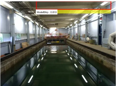
Fig. 21. Visualization of distance estimation and object
[image:9.612.337.567.528.701.2]Figure 22. Visualization of distance estimation and object recognition at the time of 231 sec in case 1. The numbers above the bounding box indicate the estimated distance, and the text below indicates the classification result and corresponding matching probability.
Fig. 23. Wrong detection in case 2 compared to case 1. The
parts where wrong recognition are marked as circles.
Fig. 24. Visualization of distance estimation and object
recognition at the time of 277 sec in case 1. The numbers above the bounding box indicate the estimated distance, and the text below indicates the classification result and corresponding matching probability.
Fig. 25. Visualization of distance estimation and object
recognition at the time of 277 sec in case 2. The numbers above the bounding box indicate the estimated distance, and the text below indicates the classification result and corresponding matching probability.
Result comparison between case 2 and case 3; focusing on dataset quality
Cases 2 and 3 have the same proposal configuration but the dataset image was different. The dataset images in case 2 were mainly consisted of the images of the same model ship that has been used in the detection test. On the other hand, the dataset image in case 3 is composed of images of completely different model ships that have not been used in the detection test. The purpose of arranging the dataset was to test the CNN’s strength that it can recognize certain object even if it has not been trained with the same image. However, there was a limit to collect enough amount of images of different model ships, so that only 303 images were contained in the dataset in case 3.
As shown in Fig. 18(c), network case 3 did not detect the model ship at the distance more than 6 m, and it misrecognised or did not recognized at all in 97.24% of the frames as described in table 7. This implies that the quality of the dataset has the greatest effect on the performance of the detection algorithm, especially CNN, and its effect is extremely critical.
3) Result comparison between case 2 and case 4; focusing on dataset quantity
Case 2 and case 4 have same proposal configuration and they both were trained with images of the model ship that has been used in the detection test. The difference between them is a number of dataset images, 1034 images for case 2 and 241 images for case 4. The purpose of this comparison is to see the influence of the dataset quantity.
As indicated in Tables 6-7, network case 4 made a result that a percentage of the well-detected frame is 61.61%, which is 7.6% lower than case 2. From this, it is considered that the amount of dataset affects the CNN. The larger the amount of dataset, it is expected that the better performance of the detection algorithm.
[image:10.612.53.284.361.534.2]Overall, the proposed algorithm was impossible to estimate over a certain distance due to disparity-based calculation in terms of distance estimation. On the object detection side, detection noise was occurred due to false recognition, but changing the proposal configuration showed a slight improvement in performance compared to the default. Due to the characteristics of CNN, the performance of the proposed algorithm was more dominantly influenced by the quality of dataset than the proposal configuration and quantity of dataset.
The aim of this research was to develop a vision-based detection algorithm for USV. For this, the Faster R-CNN is used to recognize and localize objects on frames, and the depth estimation with a stereo camera is used to estimate the distance to detected objects. In order to evaluate the proposed algorithm and to examine the factors that affect the performance of the algorithm, several case studies were carried out with model ship detection test.
First of all, the average computation time per frame was
0.33 sec, revealing that it is practical for real-time detection. When CNN is trained with high quality and quantity of dataset, it detected the model ship with a probability of almost 70% and the average distance error was within 3 m. Unlike conventional vision-based detection system, the proposed algorithm clarifies the type of object through classification so that it derives additional factors that contribute to the collision risk. It thus seems that it is possible to support the automation of the USV with low cost by simplifying existing expensive equipment. However, the proposed detection algorithm required a high quality and a large amount of dataset for high performance. In particular, the quality of the dataset has had the greatest impact on the performance. This is due to the nature of artificial intelligence that draws erroneous results when it learns with incorrect information. This is why it needs a large amount of dataset to cover this enough. Another limitation observed in this test is that it was impossible to estimate the distance over 30 m. Since the depth estimation computes the disparity based on the texture difference between the left and right frames of the stereo camera, if the texture or resolution is low, the distance estimation is limited. This limitation in this test was because the frame was taken at a resolution of 640 × 480.
The most important point for the real application of this algorithm is a large amount of high-quality image dataset of marine obstacles. Due to advances in data science, it is expected that organizations providing image databases increases then it will be able to collect these vast amounts of datasets effortlessly in the future. We plan to train the CNN by collecting image datasets of various objects that may exist in actual sea, not model ship, and to make a more powerful detection algorithm by using a high-resolution stereo camera. In addition, since the ultimate goal of the USV detection system is collision avoidance, we plan to devise a method to calculate the collision risk using the information of the type of object, direction to object, and distance to object, which are derived from the proposed algorithm.
CONCLUSIONS
We implemented object detection algorithm combining Faster
R-CNN and depth estimation with a stereo camera. The dataset for Faster R-CNN has been collected as the images of model ship used in detection test and other model ships. The Faster R-CNN has trained with that dataset for its fine-tuning. In this process, we have felt the need for object recognition that occupies a small area on the frame, so that we accordingly modified the existing default configuration of Faster R-CNN and resized the images in the dataset.
In order to examine the efficiency of the proposed algorithm and its influencing factors, Faster R-CNN has been trained in four cases by varying the quality, quantity of dataset, and proposal configuration. Test results have shown that the quality of the dataset has the greatest effect on the performance of the algorithm. In this research, the Faster R-CNN has shown almost 70% recognition ability if such dataset condition is satisfied. The distance estimation using depth estimation in this test cannot estimate the distance over 30 m. This happens because the depth estimation technique computes the disparity based on the texture of the frame. As the distance to the model ship increases, the number of pixels containing the visual information of the area decreases. On the other hand, when estimating the distance within 30 m, the average distance error has been only within 3 m. Therefore, if the resolution of the camera is high, then the depth estimation technique seems to be well worth applying.
Finally, the average computation time per frame has been
0.33 sec when computing with the above two techniques combined. Therefore, it has been confirmed that there is a possibility of real application if high quality and quantity dataset can be collected and a high-resolution stereo camera is used.
REFERENCES
Bradski, Gary, and Adrian Kaehler. 2008. Learning OpenCV: Computer Vision with the OpenCV Library. “ O’Reilly Media, Inc.”
Campbell, S., W. Naeem, and G. W. Irwin. 2012. “A Review on Improving the Autonomy of Unmanned Surface Vehicles through Intelligent Collision Avoidance Manoeuvres.” Annual Reviews in Control. Pergamon.
https://doi.org/10.1016/j.arcontrol.2012.09.008.
Dalal, Navneet, and Bill Triggs. 2005. “Histograms of Oriented Gradients for Human Detection.” In Computer Vision and Pattern Recognition, 2005. CVPR 2005. IEEE Computer Society Conference on, 1:886–93. IEEE.
Deshpande, Adit. 2016. “The 9 Deep Learning Papers You Need To Know About.” UCLA. 2016.
https://adeshpande3.github.io/The-9-Deep-Learning-Papers-You-Need-To-Know-About.html.
Eggert, Christian, Dan Zecha, Stephan Brehm, and Rainer Lienhart. 2017. “Improving Small Object Proposals for Company Logo Detection.” In Proceedings of the 2017 ACM on International Conference on Multimedia Retrieval, 167–74. ACM.
Everingham, Mark, Luc Van-Gool, Chris Williams, John Winn, and Andrew Zisserman. 2007. “The PASCAL Visual Object Classes Challenge 2007.” 2007.
Gladstone, Ran, Yair Moshe, Avihai Barel, and Elior Shenhav. 2016. “Distance Estimation for Marine Vehicles Using a Monocular Video Camera.” In Signal Processing Conference (EUSIPCO), 2016 24th European, 2405–9. IEEE.
He, Kaiming, Xiangyu Zhang, Shaoqing Ren, and Jian Sun. 2016. “Deep Residual Learning for Image Recognition.” In Proceedings of the IEEE Conference on Computer Vision and Pattern Recognition, 770–78.
Heiko Hirschmüller (Inst. of Robotics & Mechatronics Oberpfaffenhofen, German Aerosp. Center, Wessling, Germany). 2005. “Accurate and Efficient Stereo Processing by Semi-Global Matching and Mutual Information.” In Computer Vision and Pattern
Recognition, 2005. CVPR 2005. IEEE Computer Society Conference on (Volume: 2), 2:807–14. IEEE.
https://doi.org/10.1109/CVPR.2005.56.
Hirschmuller, Heiko. 2005. “Accurate and Efficient Stereo Processing by Semi-Global Matching and Mutual Information.” Computer Vision and Pattern Recognition, 2005. CVPR 2005. IEEE Computer Society Conference on 2 (2). IEEE: 807–14.
https://doi.org/10.1109/CVPR.2005.56.
Krizhevsky, Alex, Ilya Sutskever, and Geoffrey E Hinton. 2012. “Imagenet Classification with Deep Convolutional Neural Networks.” In Advances in Neural Information Processing Systems, 1097–1105.
Ren, Shaoqing, Kaiming He, Ross Girshick, and Jian Sun. 2015. “Faster R-Cnn: Towards Real-Time Object Detection with Region Proposal Networks.” In Advances in Neural Information Processing Systems, 91–99.
Shin, Bok-Suk, Xiaozheng Mou, Wei Mou, and Han Wang. 2018. “Vision-Based Navigation of an Unmanned Surface Vehicle with Object Detection and Tracking Abilities.” Machine Vision and Applications. Springer, 1–18. Simonyan, Karen, and Andrew Zisserman. 2014. “Very Deep
Convolutional Networks for Large-Scale Image Recognition.” arXiv Preprint arXiv:1409.1556.
Sinisterra, Armando J, Manhar R Dhanak, and Karl von Ellenrieder. 2014. “Stereo Vision-Based Target Tracking System for an USV.” In Oceans-St. John’s, 2014, 1–7. IEEE.
Szegedy, Christian, Wei Liu, Yangqing Jia, Pierre Sermanet, Scott Reed, Dragomir Anguelov, Dumitru Erhan, Vincent Vanhoucke, and Andrew Rabinovich. 2015. “Going Deeper with Convolutions.” In . Cvpr.
Wang, Han, and Zhuo Wei. 2013. “Stereovision Based Obstacle Detection System for Unmanned Surface Vehicle.” In Robotics and Biomimetics (ROBIO), 2013 IEEE International Conference on, 917–21. IEEE.
Wang, Han, Zhuo Wei, Sisong Wang, Chek Seng Ow, Kah Tong Ho, and Benjamin Feng. 2011. “A Vision-Based Obstacle Detection System for Unmanned Surface Vehicle.” In Robotics, Automation and Mechatronics (RAM), 2011 IEEE Conference on, 364–69. IEEE. Wang, Han, Zhuo Wei, Sisong Wang, Chek Seng Ow, Kah
Tong Ho, Benjamin Feng, and Zhou Lubing. 2011. “Real-Time Obstacle Detection for Unmanned Surface Vehicle.” In Defense Science Research Conference and Expo (DSR), 2011, 1–4. IEEE.
Woo, Joohyun. 2016. “Vision Based Obstacle Detection and Collision Risk Estimation of an Unmanned Surface Vehicle.” In 2016 13th International Conference on Ubiquitous Robots and Ambient Intelligence (URAI), 0:461–65. IEEE.
https://doi.org/10.1109/URAI.2016.7734083.
Woo, Joohyun, and Nakwan Kim. 2016. “Vision-Based Target Motion Analysis and Collision Avoidance of Unmanned Surface Vehicles.” Proceedings of the Institution of Mechanical Engineers, Part M: Journal of Engineering for the Maritime Environment 230 (4). SAGE Publications Sage UK: London, England: 566–78.