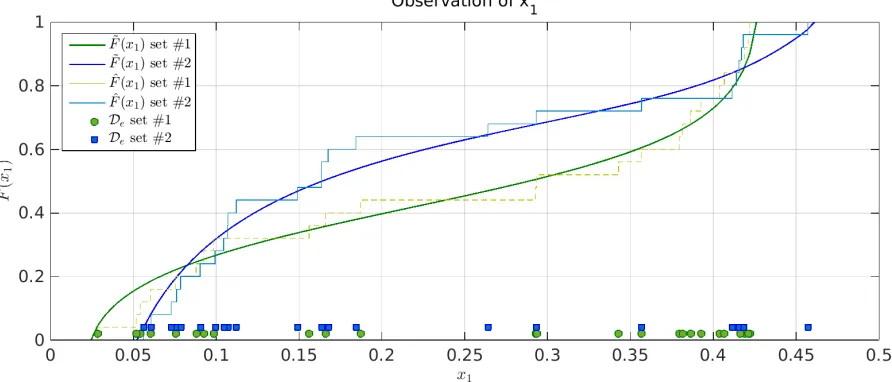
Uncertainty Management in Multidisciplinary Design of Critical Safety Systems

Uncertainty management in multidisciplinary design of

1

critical safety systems

2

Edoardo Patelli

Diego A. Alvarez

Matteo Broggi

Marco de Angelis

3

Managing the uncertainty in multidisciplinary design of safety critical systems requires 4

not only the availability of a single approach or methodology to deal with uncertainty 5

but a set of different strategies and scalable computational tools (i.e. by making use of 6

the computational power of a cluster and grid computing). The availability of multiple 7

tools and approaches for dealing with uncertainties allows to cross-validate the results and 8

increase the confidence in the performed analysis. 9

This paper presents a unified theory and an integrated and open general purpose com-10

putational framework to deal with scarce data, aleatory and epistemic uncertainties. It 11

allows to solve different tasks necessary to manage the uncertainty, such as: uncertainty 12

characterization, sensitivity analysis, uncertainty quantification and robust design. The 13

proposed computational framework is generally applicable to solve different problems in 14

different fields and numerically efficient and scalable allowing for a significant reduction of 15

the computational time required for uncertainty management and robust design. 16

The applicability of the proposed approach is demonstrated by solving a multidisci-17

plinary design of a critical system proposed by NASA Langley in the multidisciplinary 18

uncertainty quantification challenge problem. 19

∗_{Institute for Risk and Uncertainty, University of Liverpool, UK, email: [email protected]}

†_{Department of Civil Engineering, Universidad Nacional de Colombia at Manizales, Colombia}

I.

Introduction

20

In order to design safe components and systems, the explicit inclusion of uncertainties from different

21

sources is an indispensable step. In fact, under realistic conditions, these products are affected by

uncertain-22

ties, caused by the lack of sufficient knowledge and/or by natural unpredictable external events. Uncertainty

23

analysis is essential for modellers to obtain a robust representation of model predictions consistent with the

24

state-of-knowledge. If the effects of the uncertainties in the “optimized” products are ignored, these

prod-25

ucts may perform unsatisfactorily in realistic conditions; for instance, they can show a very low reliability,

26

high reparation and maintenance costs. On the other hand, in a robust design a product or system is less

27

sensitive to the uncertainties and hence, it reaches low variability of the overall performances that can allow

28

significant reductions in terms of e.g. the manufacturing and operating costs).

29

The design of safety critical systems faces very complex problems due to the presence of varying levels of

30

aleatory and epistemic uncertainty. Aleatory uncertainty is inherent in many natural systems, and therefore

31

cannot be reduced, but can be described and its effect quantified. Epistemic uncertainty is not completely

32

avoidable, since it is not possible to perfectly model or predict real world situations, although epistemic

33

uncertainty can be reduced, better characterized and quantified by using available knowledge. Despite the

34

different levels of uncertainty, decision makers still need to make clear choices based on the available

infor-35

mation. They need to trust the methodology adopted to propagate uncertainties through multi-disciplinary

36

analysis, in order to quantify the risk with the current level of information and avoid wrong decisions due

37

to artificial restrictions introduced by the modelling.

38

Multiple mathematical concepts can be used to characterize variability and uncertainty. Probability

39

distributions can be used to represent the relative frequency of a given state of the system, or they can

40

represent the degree of belief or confidence that a given state of the system exists.1 _{Often, very limited} 41

information is available, and collecting more data or samples might not be possible or too expensive. Given

42

the limitations of amount of data, quantification methods often rely on subjective judgment and assumptions

43

and it may not always seem reasonable to characterize the uncertainties in a classical probabilistic way. To

44

avoid the inclusion of subjective and often unjustified hypothesis, the imprecision and vagueness of the data

45

can be treated by using concepts of imprecise probabilities. Imprecise probability combines probabilistic and

46

set theoretical components in a unified theory allowing the identification of bounds on probabilities for the

events of interest.2 48

Random set theory is specially suited to model under the same framework uncertainty represented as

49

cumulative distribution functions (CDFs), intervals,3_{probability boxes,}4_{possibility distributions}5 _{(they are} 50

closely related to normalized fuzzy sets) and Dempster-Shafer6,7_{structures without making any implicit or} 51

explicit assumptions. In other words, random set theory is a technique that permits to model naturally the

52

aforementioned representations of uncertainty.

53

In this work, novel and efficient strategies are proposed to deal with aleatory and epistemic uncertainty.

54

Random set theory is used as a unifying theoretical framework, to model different representations of the

55

uncertainty. Additionally, the developed procedures have been implemented in an integrated computational

56

framework allowing to solve realistic problems using a number of different approaches and methodologies.

57

This provides an excellent tool for cross-validating the results obtained at each stage of the analysis and

58

hence to increase the confidence in the adopted methodology and in the results. The applicability of approach

59

is demonstrated by solving the NASA Langley multidisciplinary uncertainty quantification (UQ) challenge

60

problem.8 61

Motivation of the study

62

The development of safety-critical systems that must be designed to operate in harsh environments with a

63

wide array of operating conditions (e.g. new vehicles, aircraft, nuclear power plants etc.) is a challenging

64

problem. Furthermore, the failure of such systems might have high consequences for which quantitative

65

data is either very sparse or prohibitively expensive to collect. Hence, uncertainty management is necessary

66

to provide support to the decision makers through a series of different and interconnected analyses. For

67

instance, estimating the importance of collecting additional information allows to characterize and reduce

68

uncertainty; by performing sensitivity analysis, it is possible to identify the parameters that contribute the

69

most to the variability of the output; uncertainty propagation allows to study the effects of uncertainty on

70

the performance of the system and to identify extreme-case scenarios; finally, optimizing the design explicitly

71

taking into account the effect of uncertainties allows to design a robust system.

72

Recent reports have clearly shown that the risk assumed by the decision maker is often wrongly estimated

73

uncertainty (and descriptions of any processes used to obtain these estimates) in order to increase confidence

75

and consistency in safety predictions and encourage the development of improved methods for quantifying

76

and managing uncertainty. In this context, the NASA Langley multidisciplinary uncertainty quantification

77

(UQ) challenge problem has been addressed in order to determine limitations and ranges of applicability of

78

existing UQ methodology and to advance the state of the practice in UQ problem.9 79

The NASA challenge problem has represented a unique opportunity to test, validate and advance the

80

capability of the computational framework, namelyOpenCossan.10 _{This computational framework is able} 81

to deal with different representations of uncertainty and has been adopted to solve all the tasks proposed by

82

the challengers.

83

Since many of the employed methods are rooted on random set theory, a brief introduction of the theory

84

for the representation of the joint existence of aleatory and epistemic uncertainty is presented in Section

85

II. The developed approaches for uncertainty quantification and management are presented in Section III.

86

Section IVpresents the computational framework and some details on computational complexity. Section

87

Vsummarizes the main aspects, goals and difficulties of the NASA Langley multidisciplinary UQ challenge

88

problem as well as the results of the various tasks of the challenge problem. Finally, the potentiality and

89

applicability of the developed computational framework and the proposed approaches are discussed.

90

II.

Theoretical background

91

Random set theory is specially suited to model, under the same framework, uncertainty represented as

92

cumulative distribution functions (CDFs), intervals, distribution-free probability boxes, possibility

distribu-93

tions and Dempster-Shafer structures6,7 _{without making any implicit or explicit assumption at all.}11,12 _In 94

other words, random set theory is a technique that permits to model the aforementioned representations of

95

uncertainty. Random sets can be understood as random variables that sample, instead of points, sets (called

96

focal elements) as realizations.

97

In this context, many of the proposed solutions to the challenge problem make strong use of this kind of

98

representation. In consequence, in the following, a brief review of the main concepts of random set theory

99

that will be required in the subsequent discussion is provided. Also some new concepts developed in order

100

to solve the challenge problem will be introduced.

A. A succinct review of random set theory

102

Let us consider a universal setX 6=∅and its power setP(X). Let (Ω0, σΩ0, PΩ0) be a probability space and 103

(F, σ_F) be a measurable space whereF ⊆P(X). Arandom set Γ is a (σΩ0−σF)-measurable mapping 104

Γ :Ω0→F,α7→Γ(α). We will say that every γ:= Γ(α)∈F is afocal element whileF is a focal set.

105

Analogously to the definition of a random variable, this mapping can be used to define a probability

106

measure on (F, σF) given byPΓ:=PΩ0◦Γ−1. That is, an eventR ∈σF has the probability 107

PΓ(R) =PΩ0{α∈Ω0: Γ(α)∈ R}. (1)

The random set Γ will be also referred to as (F, PΓ). When all the focal elements ofF are singletons, then

108

Γ becomes a random variableX; hence, Γ(α) =X(α) and the probability of occurrence of the event F, is

109

PX(F) := (PΩ0◦X−1)(F) =PΩ0{α:X(α)∈ F } for everyF ∈ σX. In the case of random sets, it is not 110

possible to compute exactly PX(F) but its upper and lower probability bounds. Dempster6 defined those 111

upper and lower probabilities by,

112

LP(_F,PΓ)(F) :=PΩ0{α: Γ(α)⊆ F,Γ(α)6=∅} (2a)

UP(_F,PΓ)(F) :=PΩ0{α: Γ(α)∩ F 6=∅} (2b)

where LP(_F,PΓ)(F)≤PX(F)≤UP(F,PΓ)(F). 113

Copulas A copula is a function C : [0,1]d → [0,1] that relates a joint cumulative density functions

114

(CDFs) with its marginals, carrying in this way the dependence information in the joint CDF such that each

115

of its marginal CDFs is uniform on the interval [0,1]. According to Sklar’s theorem (see Refs. 13,14) , a

116

multivariate CDFFX1,X2,...,Xd(x1, . . . , xd) =P[X1≤x1, . . . , Xd≤xd] of a random vector (X1, X2, . . . , Xd) 117

with marginalsFXi(xi) =P[Xi≤xi] can be written asFX1,X2,...,Xd(x1, . . . , xd) =C(FX1(x1), . . . , FXd(xd)), 118

whereCis a copula. The copulaCis itself a CDF and it contains all information on the dependence structure

119

between the components of (X1, X2, . . . , Xd) whereas the marginal cumulative distribution functions FXi

120

contain all information on the marginal distributions.

121

The reader is referred to Ref. 15for an excellent introduction to copulas.

B. Random sets, CDFs, distribution-free probability boxes and intervals

123

The original definition of random sets is very general; Alvarez11,12_{showed that making the particularizations} 124

Ω0 := (0,1]d_{, σ}

Ω0 := (0,1]d∩Bd, where B stands for the Borel σ-algebra on R, and PΓ ≡µC for some 125

copula C that contains the dependence information within the joint random set, and using intervals and

126

d-dimensional boxes as elements ofF, it is enough to model possibility distributions, distribution-free

prob-127

ability boxes, intervals, CDFs and Dempster-Shafer structures or their joint combinations (for a definition of

128

joint Dempster-Shafer structure and joint random set the reader is referred to Ref. 12). Here,PΓ≡µC de-129

notes the fact thatPΓis the probability measure generated byPΩ0 which is defined by the Lebesgue-Stieltjes 130

measure corresponding to the copulaC, i.e. µC. In other words,PΓ(Γ(G)) =µC(G) forG∈σΩ0. 131

In the rest of this subsection, (Ω0, σΩ0, PΩ0) will stand for a probability space with Ω0:= (0,1],σΩ0 := 132

(0,1]∩B:=∪θ_∈B{(0,1]∩θ}andPΩ0will be a probability measure corresponding to the CDF of a random 133

variable ˜α uniformly distributed on (0,1], i.e. Fα˜(α) :=PΩ0[˜α ≤α] = α for α∈ (0,1]; that is, P_Ω0 is a 134

Lebesgue measure on (0,1].

135

1. Cumulative distribution functions 136

When a variable is expressed as a random variable on X ⊆R, the probability law of the random variable

137

can be expressed using a CDFFX (recallFX(x) =PΓ(X ≤x) forx∈X). That CDF can be represented as 138

the random set Γ :Ω0→F, α7→Γ(α) whereF is the system of focal elements Γ(α) :=FX−1(α) forα∈Ω0 139

(theinverse of the CDF FX is defined byFX−1(α) := inf{x:FX(x)≥α, α∈(0,1]}; take into account that 140

this definition uses the infimum since CDFs are weakly monotonic and right-continuous). Note that the

141

representation of the CDF as a random set only contains an aleatory component, which is given either by

142

α, or by its corresponding samplex=F_X−1(α); there is not an epistemic component in this representation.

143

2. Intervals 144

Aninterval I = [l, u] can be represented as the random set Γ :Ω0 →F, α7→Γ(α) (i.e. (F, PΓ)) defined

145

onRwhere the focal set contains the unique focal element [l, u], that is, F =Iandα∈(0,1]≡Ω0; in this

146

case,PΓ is specified by Eq. (1). In other words, all the samplings ofα∈Ω0 draw the interval [l, u]. Note

147

that the representation of intervals as a random set does not contain an aleatory component, inasmuch as

it does not matter which valueαtakes, because all α-s map to the same focal element I. In this case, the

149

epistemic component is given by the interval itself,I.

150

3. Probability boxes 151

A probability box or p-box (term coined by Ferson et al.4₎

F , F

is a set of CDFs {F : F ≤ F ≤ 152

F , F is a CDF}, delimited by upper and lower CDF bounds F and F : R → [0,1], which collectively

153

represent the epistemic uncertainty about the CDF of a random variable. This class of functions may not

154

have additional restrictions or may belong, as well, to a reduced class of CDFs; using that discrimination,

155

probability boxes can be naturally grouped into two disjoint groups: free and distributional.

156

Distribution-free p-boxes Distribution-free p-boxes (also known as non-parametric p-boxes) appear

157

when the CDF of a random variable cannot be specified precisely, given that the CDF family is unknown; in

158

this case only the upper and lower CDF boundsF andF bounds of the probability box are specified. These

159

bounds can either be defined in advance or can be estimated using for example the methods listed in Zhang

160

et. al.16 _{and references therein. Note that distribution-free p-boxes do not make any assumption about the} 161

family or shape of the uncertain CDFs that belong to the p-box.

162

There are two alternatives but equivalent methods to represent distribution-free p-boxes using random

163

set theory.

164

The first method was proposed in Refs. 11,12. Using this method, a distribution-free probability box 165

delimited by lower and upper CDF bounds F and F can be represented as the random set Γ : Ω0 → 166

F, α 7→ Γ(α) (i.e. (F, PΓ)) defined onR where F is the class of focal elements Γ(α) := hF , Fi−1(α) :=

167

h

F−1(α), F−1(α)iforα∈(0,1]≡Ω0 withF−1(α) andF−1(α) denoting the inverses ofF andF andPΓ is

168

specified by Eq. (1).

169

The second alternative method, proposed here, considers a random variable which follows a CDFF with

170

parametersθi that belong to the intervalIifori= 1,2, . . . , m(i.e. F(·;θ1, θ2, . . . , θm)). This representation 171

is in comparison to the first method, which models a p-box using only its lower and upper CDF boundsF and

172

F. Using the random set representation, a focal element of the probability box

F , F

can be represented

173

as the image through the functionF−1 _{of the input intervals{I}

i:i= 1,2, . . . , m} together with the sample 174

of α which is a uniform random variable on (0,1] ≡ Ω0. In consequence, it can be represented as the

random set Γ : Ω0 → F, α 7→ Γ(α) (i.e. (F, PΓ)) defined on Rwhere F is the system of focal elements

176

{F−1_{(α; I}

1, I2,· · · , Im) :α∈Ω0}and PΓ is specified by Eq. (1). Observe that each focal element has an

177

aleatory componentαand an epistemic component in the Cartesian product

×

This representation of distribution-free p-boxes shows that for a single realization of the aleatory

com-179

ponent α, a focal element contains the image through F−1 _{of all the possible combinations of values of}

180

the intervals for the parameters of the parental CDF F. It derives from the fact that a focal element

181

is defined as:

F , F−1

(α) =

x:F(x) =α, F ∈

F , F , F−1(α) = infθ∈×m i=1IiF−

1_(α;θ

1, . . . , θm) and 182

F−1(α) = supθ∈×m i=1IiF

−1_(α;θ

1, . . . , θm). 183

Note that only distribution-free probability boxes can be represented using random set theory. However,

184

in the analysis of the challenge problem a different approach has been used to represent distributional

185

probability boxes as will be explained in the following lines.

186

Distributional p-boxes and the double loop Monte Carlo strategy Distributional p-boxes

187

(also known asparametricp-boxes) appear when there is uncertainty in the representation of the parameters

188

of a given CDF (hereafter called theparental CDF.) These parameters are imprecisely specified as intervals.

189

For instance, consider a quantity that is known to be Gaussian with mean within the interval [1,2] and

190

standard deviation somewhere in [3,4]; Ferson et. al.4 _{describes how to obtain such probability boxes. All} 191

CDFs that are normal and have means and standard deviations inside these respective intervals will belong

192

to this probability box. The upper and lower CDF boundsF and F of the p-box enclose many non-normal

193

distributions, but these would be excluded from the p-box by specifying the normal CDF as the parental 194

distribution family.

195

According to the second representation of distribution-free p-boxes, the focal element corresponding to

196

a realization αof the aleatory component contains the image through F−1 _{of all possibleθ ∈}

×

i=1Ii. As 197

consequence, a set of focal elements of the probability box would be a family of intervals each of them being

198

a mapping of

×

intervals the points that would belong to some CDF. For this reason, random set theory can not be used to

200

model distributional p-boxes.

201

Distributional p-boxes can be dealt with using a double loop Monte Carlo strategy, in which the outer

202

using the principle of maximum entropy, we will assume a uniform distribution in

×

has been used tosolve some of the tasks of the challenge problem. Please note that the outer loop can be

205

used to drive an optimization/search process in

×

it is not necessary to assume a uniform distribution in

×

C. Sampling from a random set

208

A sample from a random set is simply obtained by generating anαfrom a uniform distribution on (0,1] and

209

then, retrieving the corresponding focal element Γ(α); for example, for sampling from a

distributional-210

free probability box an α uniformly distributed in (0,1] is drawn and then its corresponding “α-cut”

211

h

F−1(α), F−1(α)i is obtained. In the case of multivariate random sets, a sample α ∈ Ω0 is drawn from

212

the copula C that models the dependence between the input variables . Then, the corresponding marginal

213

focal elements are obtained and combined as explained in the next subsection. Take into account that n 214

samples of a random set form the Dempster-Shafer structure (Fn, m); hereFn denotes the set of all sampled 215

focal elements; the basic mass assignmentm associated to each focal element is equal to 1/n; note that a

216

Dempster-Shafer structure is itself a finite random set.11,12

217

Samples from distributional p-boxes can be obtained resorting to a double Monte Carlo loop as explained

218

in the previous Section.

219

D. Combination of focal elements

220

After sampling each input variable, a combination of the sampled focal elements is carried out. Usually,

221

the joint focal elements are given by the Cartesian product

×

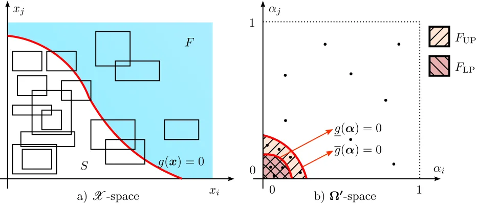
variables, γi := Γi(αi) are the sampled focal elements from every input variable (that is, γi represents a 223

sampled marginal focal element). Some of these γi are intervals, some other, points. Inasmuch as every 224

sample of a input variable can be represented byγi or by the corresponding αi, the joint focal element can 225

be represented either by thed-dimensional boxγ:=

×

(see Figure1).

a)

X

_-space

_b)

_Ω

_-space

F

F

x

x

α

α

F

S

₀

0

1

1

g

(

x

) = 0

g

(

α

) = 0

g

(

α

) = 0

Figure 1: Focal elements in theX (Panel a) and in theΩ0-space (Panel b), respectively. The focal elements

are the realizations of input variables which are depicted either as the pointsαin theΩ0-space or as

(multi-dimensional) boxes, corresponding to the focal element Γ(α), in the X space. The figure (a) shows also the

failure surface,g(x) = 0, that defines the safeS and failureF domains. In theΩ0-space (b) are defined the

regionsFLPandFUPtogether with the failure surfacesg(α) = 0 andg(α) = 0, whereg(α) := minx∈Γ(α)g(x) and g(α) := maxx∈Γ(α)g(x). Those boxes inX which contain at least one point of the failure region F have a correspondingα point in the regionFUP; while those boxes inX which are completely contained in the regionF have a correspondingαpoint in the regionFLP.

E. The epistemic and the aleatory spaces

228

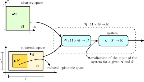
Along this paper, two spaces are defined for modelling the aleatory and the epistemic uncertainties and

229

which are called thealeatory space Ω and theepistemic space Θ, respectively (see Figure2).

230

The aleatory space A sample from a random set is obtained by drawing anα∈Ω0 from the copulaC.

231

Since a sample from an interval does not contain an aleatory component, if we strip from spaceΩ0all those

232

components which belong to intervals, then a subspaceΩof Ω0 is obtained. The subspaceΩcontains only

233

probabilistic information without spurious random variables. This set is called from now on the aleatory 234

space Ω. Without loss of generality all copulas in our discussion will be defined onΩ, and all subsequent

235

discussion will be performed with respect to the setΩ.

The epistemic space The epistemic spaceΘ is formed by the Cartesian product of all intervals{Ii, i= 237

1,2, . . . , q} that contain epistemic uncertainty, that isΘ=

×

reduced when additional information is available, we will assume that a pointθ∗∈Θin the epistemic space

239

will represent the “true uncertainty model”, which will result once all epistemic uncertainty is removed from

240

Θ. When new information is available, the epistemic space will shrink to a subset of it called the reduced 241

epistemic space.

242

For example, let’s consider a problem with four input variables: two correlated random variablesXandY 243

modelled as a bivariate normal distribution and two independent variablesW andZ which are modelled by

244

the intervalsIW andIZ, correspondingly. The joint CDF ofXandY is defined by the mean vector [µX, µY]T, 245

variances [σ2X, σ

2

Y]

T _{and a Pearson correlation coefficient ρ}

XY. If we assume that all those five parameters 246

are also unknown and represented by intervals, namely, IµX, IµY, Iσ2

X, Iσ2Y and IρXY, respectively, then,

247

the aleatory space Ω is (0,1]2 _whileΩ0 _{is (0,1]}4_{; in addition, a Gaussian copula is defined on the aleatory}

248

space Ω. Finally, the epistemic space Θ is a seven-dimensional space formed by the Cartesian product

249

IµX ×IµY ×Iσ2

X ×Iσ2Y ×IρXY ×IW ×IZ. Notice that the pointθ

∗ _{belongs to that space.}

250

F. The system representation as a function of the aleatory and the epistemic uncertainty

251

Let us denote by G : X → _R a function that represents the system; this function maps from the input

252

spaceX of input variables to the real line and letW :Ω×Θ→X be a function which returns the point

253

in Γ(α) after reducing the epistemic uncertainty in Θto θ. The function W exists only if the random set

254

Γ models intervals, CDFs, p-boxes or their joint combination. This function does not exist if Γ models

255

Dempster-Shafer structures or possibility distributions, but this is not the case in this paper. Note on the

256

one hand, that the image ofΘthroughW(α;·) is the focal element Γ(α); on the other hand, the image ofΩ

257

throughW(·;θ) can be modelled as a CDF with parameter vectorθ, that is,F(·;θ). Take into account that

258

the definition of function W uses, in the case of CDFs and p-boxes, the inverse CDF of the input variable

259

in consideration.

260

We will define the function H:Ω×Θ→RasH=G ◦ W, that is,Hrepresents the system as well, but

261

its domain is the Cartesian product of the aleatory and epistemic spaces (see Figure2).

reduced epistemic space

aleatory space

epistemic space

realization of the input of the

system for a given

α

_and

θ

system

α

θ

0

1

1

I

I

α

α

θ

Ω

Θ

W

:

Ω

×

Θ

→

X

_G

_:

X

→

_R

H

:

Ω

×

Θ

→

_R

Figure 2: Representation of the aleatory and epistemic spaces and their propagation through the model.

Hereθ∗represents thetrue uncertainty model after all epistemic uncertainty has been removed. The subset

of the epistemic space that appears after new information is available is the reduced epistemic space. The

functionWproduces a realization for a givenαandθ; this output becomes the input for the systemG. The

composition of both functions forms the functionH.

G. Mapping of a focal element through a system: the extension principle of random sets

263

The capability to propagate intervals, CDFs, p-boxes, and their combination through a system represents

264

the core of the developed computational framework. In order to find the image of a focal element,γi⊆X, 265

through a function G : X → R, the extension principle of random sets is used (this principle states how

266

to propagate a random set through a function – see Ref. 17). This can be done by means of optimization

267

methods,18 _{sampling methods,}19_{a vertex method,}20_{or the interval arithmetic method.}21,3 _{In the following,} 268

the optimization and the sampling methods will be explained in detail, since both methods have been

269

employed to solve the NASA UQ challenge problem.

The optimization method If a focal elementγi:= Γ(αi) is connected and compact andG is continuous, 271

then the image of the setγi throughG, can be calculated as 272

G(Γ(αi)) =

G(αi), G(αi)

(3)

where,

273

G(αi) := min

xi∈Γ(αi)

G(xi) G(αi) := max

xi∈Γ(αi)

G(xi) ; (4)

are limit state functions defined in Ω. Using the functionHdefined in SectionF, Eqs. (4) can be written

274

as an optimization over the epistemic space:

275

G(αi) := min

θ∈ΘH(αi,θ) G(αi) := maxθ∈ΘH(αi,θ). (5)

This approach is usually employed when G is a nonlinear function of the system parameters. The main

276

drawback of this method is that it requires a high computational effort in a complex and large scale system.

277

The sampling method (random search) The image of the focal element γi through G can also be 278

estimated using a sampling technique (this should not be confused with the double loop simulation used

279

to deal with distributional p-boxes). Remembering that the focal element γi is a multi-dimensional box; 280

random samples can be generated inside that box and then they are mapped through G; then Eqs. (4)

281

are approximated by the smallest and largest values of the images of those samples. This method is easy

282

to implement but it requires huge number of samples (due to the curse of dimensionality). The sampling

283

method gives does not guarantee that the true minimum and maximum are identified even using a very large

284

number of samples.

285

III.

Proposed approach for uncertainty management and quantification

286

The robust design of safety-critical systems requires not only the explicit treatment of different forms and

287

representations of uncertainty but also, performing a number of different tasks. Generally, the design of such

288

systems requires inputs and criteria of different disciplines and one of the main challenges in uncertainty

289

management is how to propagate the uncertainty and understand how the uncertainty in one field affects

290

other disciplines. More specifically,

• the first task required is to refine the current uncertainty model using new available information. This

292

task is often called model updating (see e.g. Refs. 22,23);

293

• usuallysensitivity analysisis performed for the identification of those parameters whose uncertainty is

294

the most/least consequential. This allows to drive the collection of new data and information focusing

295

on those parameters that affect mostly the variability of the outputs;

296

• thepropagation of mixed aleatory and epistemic uncertainties of the refined/improved model and the

297

extreme-case system performance assessment are performed in order to identify the combinations of

298

parameters that lead to the worst performance;

299

• finally the design in the presence of uncertainty is achieved. This task is computationally demanding

300

since it requires the propagation of the uncertainty through the system for each candidate solution.

301

Different tools and approaches exist for uncertainty quantification and characterization that can be

302

potentially used in the design of safety critical systems. Each method is based on some assumptions that

303

often cannot be verifieda priori. Moreover, the simulation strategies are able to produce accurate results

304

only if the right set of parameters is selected and this often cannot be verified. Finally, the numerical

305

implementation might contain errors.

306

For these reasons, it is necessary to perform the analysis using different strategies and hypotheses in

307

order to be able tocross-validatethe results. Hence, different strategies implemented in a flexible and open

308

computational framework are briefly summarized in the next sections.

309

A. Model updating

310

The aim of model updating is to reduce the epistemic uncertainty on the output of the modelx=H(α;θ)

311

based on the availability of a limited set of data (observations) De := {xek : k = 1,2, . . . , ne}. These 312

observations of the “true uncertainty model”θ∗∈Θcan be used to improve the uncertainty model, i.e. to

313

reduce the original intervals of the epistemic uncertainties by excluding those combinations of parameters

314

that fail to describe the observations as shown in Figure2. Two different approaches will be used for model

315

updating: a non-parametric model based on some statistical tests and a Bayesian method.

Along the rest of this paper hats ( ˆF) and tildes ( ˜F) will be used for referring to empirical CDFs and a

317

kernel density estimations of CDFs, respectively.

318

1. Non-parametric statistic method based on the Kolmogorov-Smirnov test 319

A simple and fast approach to improve the uncertainty model is based on the comparison of the CDFs of

320

the observations of the true uncertainty model and those obtained by means of random combinations of the

321

input parameters in order to identify tighter intervals which form a reduced epistemic space and which are

322

in agreement with the observations.

323

Let us consider the epistemic spaceΘof the involved variables. Random realizationsθi in the epistemic

324

spaceΘare generated assuming, for example, a uniform PDF onΘ(in agreement with the Laplace’s principle

325

of indifference). Thereafter the points{αj, j= 1,2, . . . , n}are sampled from the aleatory spaceΩaccording

326

to the copulaC (Nelsen15 _{provides methods to do it), in order to simulatenobservations from the system} 327

Hasxi

j=H(αj,θi). For a single realizationθi, the Kolmogorov-Smirnov statistic, which is defined as 328

Di= sup x

|Fˆ(x|θi)−Fˆe(x)|, (6)

is used to measure the similarity between the CDFs obtained with the sampled set{xi

j, j = 1,2, . . . , n}and 329

the set of observationsDe. Here ˆF(·|θi) and ˆFeare the empirical CDFs obtained using the random samples 330

drawn according to the epistemic parametersθiand the provided experimental data, respectively.

331

The Kolmogorov-Smirnov test is used to obtain confidence limits on ˆF(·|θi) by choosing different critical

332

values of the test statistic D. This implies that a band of width ±D around ˆFe(x) will entirely contain 333

ˆ

F(·|θi) with probability 1−c. This allows to identify those combinations of epistemic parameters such that

334

P(Di > D) = c. c = 0 means that all the CDFs ˆF(·|θi) are accepted and the refinement of the input 335

intervals is not possible, whereasc = 1 implies that ˆF(·|θi) comes exactly from the same model that has

336

generated the target distribution ˜Fe(x), i.e. no epistemic uncertainty is present. 337

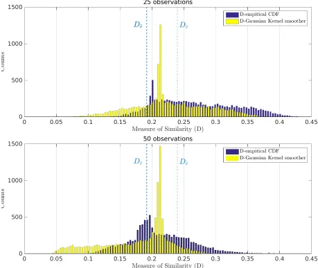
The selection of D is a critical task and generally depends of the amount of available information (i.e.

338

number of observations). A practical approach is to use two different data sets that come from the same

339

process to estimate the critical level of the measure of similarityDvˆ(using Eq. (6)). The computed validation

340

distance Dˆv can be used to set the required confidence level, accepting all the combinations of epistemic 341

parameters withDi< Dvˆ. When an independent validation data set is not available, a cross validation data

set can be constructed to test the model in order to limit problems such as overfitting. This cross validation

343

data set can be obtained by means of re-sampling techniques.24 _{Cross-validation is important to protect} 344

against hypotheses suggested by the data25 _{specially where further samples are costly or simply impossible} 345

to collect.

346

The non-parametric approach based on the Kolmogorov-Smirnov test is a simple and fast method for

347

performing uncertainty characterization (and model updating). However, it is important to keep in mind

348

the limitations of the approach. In fact, the method assumes that the measure of similarityDiis distributed 349

according to the Kolmogorov distribution,26 _{which is strictly true only for large sample sets. It is possible} 350

to use some smoother techniques such as the Gaussian kernel density estimation to overcome this limitation.

351

Gaussian kernel density estimates forDeare given by

352

˜

Fe(x) =

1

nσ√2π

Z x

−∞ ne

X

j=1

exp −1

2

_x0_−xe

j σ

2!

dx0; (7)

hereσstands for the standard deviation of the Gaussian kernels that represents the smoothing parameter,

353

proportional to the so-called bandwidth. Assuming x is a continuous random variable, for ne → ∞ the 354

Gaussian kernel density estimate converges to the true underlying density. The support of the associated

355

PDFs ˜fe(x) (i.e. {x: ˜fe(x)> 0}) and the bandwidth of the kernel have strong influence on the resulting 356

estimate. We suggest to use the approach in Ref. 27 to estimate the support of the PDF and Silverman’s

357

rule of thumb28 _{to estimate the bandwidth of the kernels. Using realizations from Eq. (7) the measure of} 358

similarity can be calculated via Eq. (6) where ˆFe(x) is replaced by ˜Fe(x). Please note that the Gaussian 359

kernels can be used to define a new critical measure level indicated withD˜v. 360

To summarize, the following pseudo-algorithm is used:

361

1. Estimate the parametersσand the Gaussian kernel CDF ˜Feusing Eq. (7); 362

2. EstimateDvˆandD˜v; 363

3. Generate realizations on the epistemic space, θi;

364

4. Drawnpoints from the aleatory spaceΩ, using copulaC; we will call these samples{αj:j= 1, . . . , n};

365

5. Evaluate the model xi

6. Estimate the empirical CDF ˆF(·|θi) of the set of samples{xi

j, j= 1,2, . . . , n}; 367

7. Using Eq. (6), compute the measure of similarityDi; 368

8. IfDi< D˜v(orDi< Dˆv) collectθi. The set of collected points identify a reduced space in the original 369

epistemic space.

370

2. Bayesian updating on the epistemic space 371

Bayesian inference is a statistical method in which the Bayes’ rule is used to update the probability estimate

372

for a hypothesis as additional information is available.

373

Suppose we are given a set of observed data points De:={xe

k:k= 1,2, . . . , ne}called theevidence, and 374

which are sampled from a PDF p(·;θ∗) which belongs to a certain family of PDFs{p(·;θ) :θ∈Θ} called

375

theparametric model. The idea of Bayesian inference is to update our belief about the vector of parameters

376

θ provided thatθ∗, the true set of parameters of the PDF, is unknown. Bayes’ theorem updates that belief

377

using two antecedents:

378

• aprior PDFp(θ), which indicates all available knowledge aboutθ∗before the evidenceDeis observed;

379

• and the likelihood function P(De|θ), which is a function related to the probability of observing the 380

samplesDeassuming that the true parameter underlying the model PDFp(x;θ) isθ; it is defined as

381

P(De|θ) =

ne

Y

k=1

p(xe

k;θ), (8)

when a set of independent and identically distributed observationsDe is available. Please note that

382

in practice (i.e. for the numerical implementation) the log-likelihood is used instead of the likelihood.

383

The updated belief about the vector of parameters θ after observing the evidence De, is modelled by the

384

so-calledposterior PDFp(θ|De) which is calculated by: 385

p(θ|De) = P(De|θ)p(θ)

P(De)

; (9)

where the probability of the evidence,

386

P(De) =

Z

Θ

can be understood as a normalizing constant. Bayesian updating hopes that after using the evidenceDe 387

the posterior PDFp(θ|De) is sharply peaked about the true value ofθ∗. We will update our belief about the

388

true set of parametersθ∗∈Θ propagating the evidence through the Bayes’ equation numerically. Samples

389

of the posterior PDF can be generated without the necessity to evaluatep(θ|De), using an algorithm called 390

Transitional Markov Chain Monte Carlo (TMCMC).29 391

As the prior PDF, we will use a uniform distribution on the epistemic space Θ, that isθ∼Unif(Θ), in

392

accordance to the Laplace’s principle of indifference (or more generally, the principle of maximum entropy).

393

Different likelihood functions can be used, based on different mathematical assumptions; in the following

394

two methods will be proposed: a method that used a kernel density estimator to approximatep(·|θi) and a

395

approximate Bayesian computational method.

396

Bayesian computational method In this case, the likelihood is estimated through kernel density.

As-397

suming that the samples De were drawn from p(x;θi), the likelihood P(De|θi) is defined in the following

398

way:

399

1. Drawnpoints,{αj :j= 1, . . . , n}, from the aleatory spaceΩ, using copulaC;

400

2. Calculatexi

j :=H(αj;θi) forj= 1, . . . , n; 401

3. Using kernel density estimation and the samples {xi

j :j = 1, . . . , n}, estimate the CDF ˜F(·|θi) and 402

its associated PDF ˜p(x|θi) ≡ p(x;θi). This step is required because ˜p(x|θi) cannot be obtained

403

analytically;

404

4. Calculate the likelihood functionP(De|θi) as in Eq. (8). 405

Approximate Bayesian computational method The likelihood calculated by means of the “Bayesian

406

computational method” applies Bayes’ theorem directly and without strong assumptions. However it requires

407

a large number of model evaluations and a relative larger data set to converge.30 _{Recently, approximate} 408

Bayesian computational methods have been proposed to reduce the computational costs of the expensive

409

or intractable likelihood function.31,32 _{The likelihood can be for instance approximated with the following} 410

expression:

411

P(De|θi) =

ne

Y

k=1 1

√

2πσexp −

1 2

δk σ

2!

whereδkis the absolute value of the difference between the empirical CDF ˆF(·|θi) obtained for an individual 412

realizationθiof the epistemic spaceΘ, evaluated at each point{xe

k, k= 1,2, . . . , ne}and the empirical CDFs 413

of the experimental datasetDe, that is: 414

δk =

ˆ

F(xk|θi)−Fˆe(xek)

(12)

fork= 1,2, . . . , ne.Please note that the Bayesian updating approach is generally applied to identify a fixed 415

estimate of θ as close as possible to θ∗. Here, the approach has been used to identify a reduced epistemic

416

space containing the true values of the unknown parameters. If a constantσis used, the Bayesian updating

417

formulation, here introduced, is equivalent to a minimization in the least square sense of the distance between

418

the CDFs ˆF(·|θi) and ˆFe. However the value ofσis unknown and hence it represents an additional parameter 419

that needs to be estimated.33 420

This last approach is indeed based more on practical considerations than on a sound mathematical basis,

421

and is open to criticisms since the differences δk are assumed to be independent and normally distributed 422

with zero mean and unit variance, and that even thoughδk is normally distributed, it will only take values 423

in the interval [0,1] since the CDF ranges between 0 and 1.

424

Using the above defined prior PDF and likelihood functions, the TMCMC algorithm29 _{is employed in} 425

order to find samples of the posteriorp(θ|De). The likelihoodP(De|θi) is calculated, using the approximate

426

Bayesian computational method, by the following procedure:

427

1. Drawnpoints ({αj:j= 1, . . . , n}) from the aleatory spaceΩ, using copulaC;

428

2. Calculatexi

j :=H(αj;θi) forj= 1, . . . , n; 429

3. Using the samples{xi

j:j= 1, . . . , n}, estimate the empirical CDF ˆF(·|θi); 430

4. Computeδk=

Fˆ(x

e

k|θi)−Fˆe(xek)

at each pointx

e k ∈ De; 431

5. Calculate the likelihood functionP(De|θi) as in Eq. (11).

432

B. Sensitivity analysis

433

The aim of sensitivity analysis is to identify and rank the parameters that contribute mostly to the variability

434

of the output of a system H. Two approaches can be used: the Hartley-like measure of nonspecificity and

the global sensitivity analysis based on Sobol’ and total sensitivity measures. Both approaches can be used

436

to perform global sensitivity analysis in presence of epistemic uncertainty.

437

1. Nonspecificity technique 438

Before delving into this method of sensitivity analysis, a small introduction to the nonspecificity measure is

439

presented.

440

The nonspecificity, proposed by Klir and coworkers,34,35 _{is a measure of the amount of information} 441

required to remove the epistemic uncertainty; it is used in cases when we have to select a unique element

442

from a set, but we are totally indifferent about which element of the provided ones to choose.

443

The nonspecificity is based on the so calledHartley-like measure, which for ad-dimensional box (or focal

444

element)A=

×

HL(A) = log2

d

Y

i=1

(1 +ui−li)

!

. (13)

The nonspecificity of a random set with an infinite number of focal elements is given by (see Ref. 36):

446

HL((F, PΓ)) =

Z

Ω

HL(Γ(α)) dC(α); (14)

two special cases of Eq. (14) are:

447

• the nonspecificity of a Dempster-Shafer structure (Fn, m) with focal setFn={A1, . . . , An}and basic

448

mass assignmentm:

449

HL((Fn, m)) = n

X

i=1

HL(Ai)m(Ai); (15)

• the nonspecificity of a distribution-free probability boxhF , Fi:

450

HL(hF , Fi) =

Z 1

0 log2

1 +F−1(α)−F−1(α)dα. (16)

The nonspecificity is a measure of epistemic uncertainty, and in consequence, it is useful for assessing the

451

variability of the output due to the epistemic uncertainty in the input of the model.

452

The method, which is detailed in Ref. 37, calculates a Dempster-Shafer structure that is the result of

453

propagating the epistemic uncertainty through the systemH(using the extension principle for random sets).

454

Then, the Hartley-like measure of nonspecificity of that output Dempster-Shafer structure is evaluated. More

455

specifically:

1. n samplesαi ∈Ω are drawn from copula C. Thereafter, the image of the focal elementαi through

457

H is calculated by means of Eq. (5) as [minθ∈ΘH(αi,θ), maxθ∈ΘH(αi,θ)]. This set of n focal 458

elements is used to construct a Dempster-Shafer structure (Fn, m) (as explained in Section II-C) 459

which represents the propagation of the aleatory and epistemic uncertainty through the system. The

460

basic mass assignmentm of each focal element is 1/n.

461

2. Compute HLunpinched= HL((Fn, m)) according to Eq. (15). 462

3. Consider a set of points {pr: 0≤p1 < p2 < . . . < pr < . . . < pz ≤1}which are evenly distributed in 463

the interval [0,1].

464

4. For each pointpr, do the following: 465

(a) Each interval,Ij = [lj, uj] that forms the epistemic spaceΘ, is pinched (or reduced) to the value 466

given by lj+pr·(uj−lj), while leaving all other intervals unchanged (take into account that 467

pinching of groups of input variables can be performed as well). After pinching the j-th input

468

variable, a subset ofΘ, namelyΘrj, which includes the pinched inputs is formed. 469

(b) nsamplesαi∈Ωare drawn from copulaC; thereafter, the image of the focal elementαithrough

470

His calculated by means of Eq. (5) as

minθ∈ΘrjH(αi,θ), maxθ∈ΘrjH(αi,θ)

. This set ofn 471

focal elements is used to construct a Dempster-Shafer structure (Frj

n , m) for each pinching (as 472

explained in SectionII). The basic mass assignmentmof each focal element is 1/n.

473

(c) The nonspecificity HLrj := HL((Fnrj, m)) of each of those output Dempster-Shafer structures is 474

computed, as in Eq. (15).

475

(d) The nonspecificity measure of the output Dempster-Shafer structure is normalized against the

476

nonspecificity measure computed before pinching. In this way, the indexIrj= HLrj/HLunpinched 477

is calculated.

478

5. The indexIjis calculated as the mean square of all indexesIrj(remember that E[Ij2] = E[Ij]2+Var[Ij]); 479

those indexes are ranked according to their mean square.

480

Ij is used as a measure of the propagation of the epistemic uncertainty to the output of the systemH. 481

j. The mean squared has been chosen as a ranking criterion in order to account for not only the bias but also

483

the variance of the estimator. Note that a precise estimation of Ij is not necessary, since only the ranking 484

of the variablesIj is required; therefore,nis usually a small number. 485

2. Global Sensitivity analysis 486

The second approach is based on global sensitivity analysis to estimate the Sobol’ and the total indices.38 487

The global sensitivity approach cannot be applied directly to solve the problems where the uncertainty is

488

described as a distributional/free p-boxes and intervals. In fact, this method requires the exact knowledge

489

of the PDF of the input variables and the variance of a measurable model output. In consequence, an

490

alternative mathematical model toH(as defined in SectionII-F) has to be defined in the next.

491

Consider a modelH∗_{:Θ→R, that is,Y =H}∗_{(θ), whereθ= [θ}

1, . . . , θq] is a vector of random variables 492

andY is a chosen univariate model output.

493

Let us associate Θ with the epistemic space; for a given value of θj ∈Θ, the function H∗ returns the

494

area between a CDFF(·|θj) and a reference CDF F(·|θ):

495

yi:=H∗(θi) :=

Z +∞

−∞

|F(x|θi)−F(x|θ)|dx; (17)

here θ denotes the center of gravity of Θ (in other words,θ is a vector formed by the mean value of each

496

input epistemic parameter), andF(·|θ) represents the CDF obtained after mapping all aleatory uncertainty

497

through the system H, for a given set of epistemic parameters θ. Since the global sensitivity analysis is

498

based on the variance decomposition, any reference CDF can be used in the modelH∗_.

499

The procedure to estimate the empirical CDF ˆF(·|θ) as an approximation toF(·|θ) is as follows:

500

1. Drawnpoints ({αj:j= 1, . . . , n}) from the aleatory spaceΩ, using copulaC;

501

2. Evaluate the model xi

j :=H(αj;θ) forj= 1, . . . , n; 502

3. Estimate the empirical CDF ˆF(·|θ) of the set of samples{xi

j, j= 1,2, . . . , n}. 503

Using the above procedure, a sample from the random variableY, namelyyi can be estimatedby means 504

of Eq. (17) for each realization of inputθiby using the empirical CDFs ˆF(·|θ) and ˆF(·|θ). Please note that

505

value (yi =E(x|θi)) or a quantile of a distribution, it is not necessary to evaluate Eq. (17) but the model 507

output can be used directly (see SectionB-2).

508

Finally, the first order Sobol’ indices are calculated as follows39 509

Si=

Varθi[Eθ∼i(Y|θi)]

Var[Y] (18)

where Var[Y] represents the unconditional variance of the quantity of interest and Varθi[Eθ∼i(Y|θi)] the

510

variance of conditional expectation. Thetotal sensitivity index,Ti, measures the contribution to the output 511

variance ofθi of the input factors including all interactions with any other input variables, 512

Ti= 1−

Varθ∼i(Eθi(Y |θ∼i))

Var(Y) . (19)

Note that unlike the first order indices, the sum of total indices can exceed one.

513

The proposed approach allows to decompose the variance of the output Y into parts attributable to

514

the variance of the input variablesθ; in other words, it allows to identify and rank the contribution of the

515

epistemic uncertainty, i.e. interval of the parameters, on the p-boxes of quantity of interest. The magnitude

516

of the sensitivity indices are proportional to the contribution to the output variance, i.e. input factor

517

associated with a large sensitivity index contributes most to the variance of the output. Hence, adopting the

518

approach proposed here, the global sensitivity analysis allows us to identify the contribution of the epistemic

519

uncertainty of input factors on the variance of the model.

520

Different techniques exist to compute the sensitivity indices such as the extended-“Fourier Amplitude

521

Sensitivity Test” (FAST)40,41_{and the Saltelli’s method.}38 _{The FAST method allows to estimate first order} 522

Sobol’ indices, whereas Saltelli’s method computes also the total indices.

523

C. Uncertainty Propagation

524

The focus of the uncertainty propagation analysis is to quantify the effect of the uncertain model parameters

525

on quantities of interest such as the mean, variance and quantiles of the system’s response or its failure

prob-526

ability. The generalized probabilistic model makes the UQ rather challenging task in terms of computational

527

cost. The challenge is to compute the lower and upper bounds of the quantities of interest. Monte Carlo

528

method remains the most versatile and simple tool to propagate epistemic and aleatory uncertainty.

1. Optimization in the epistemic space (standard approach) 530

In this approach, the quantity of interest (e.g. mean or failure probability estimation) defines the objective

531

function; and the bounds on that objective function are calculated by means of a global search in the

532

epistemic spaceΘ. On one hand, the lower and upper bounds of the mean are obtained as:

533

µ= min

θ∈Θµ(θ) µ= maxθ∈Θµ(θ) (20)

where the mean of the response model is given by:

534

µ(θ) =

Z

Ω

H(α;θ) dC(α). (21)

On the other hand, the lower and upper bound of the failure probability, defined as the excedance of a

535

critical threshold levelHcrit _{of the model response, are obtained as} 536

Pf = min

θ∈ΘPf(θ) Pf = maxθ∈ΘPf(θ); (22)

herePf(θ) stands for the failure probability, that is, 537

Pf(θ) :=

Z

Ω

I[H(α;θ)>Hcrit] dC(α). (23)

538

Monte Carlo method is used to calculate the bounds Eq. (20) and Eq. (22), by means of a double loop

539

simulation:

540

• The outer loop drives an optimization/search process in the epistemic space Θ to identify the lower

541

and upper bounds Eq. (20) and Eq. (22). This search is performed by Monte Carlo sampling taking

542

into account that this optimization method is very inefficient in high dimensional spaces since the

543

search space grows exponentially with the number of variables. Better optimization strategies such as

544

Genetic Algorithms can also be adopted as shown in SectionV-C.

545

• The inner loop propagates the aleatory uncertainty and estimates the statistical quantities of interest

546

(e.g. expected value, failure of probability, CDF, etc). In this way, severalαj are sampled from copula

547

C in order to estimate integrals of Eq. (21) and Eq. (23). Take into account that this Monte Carlo

548

integration in the aleatory spaceΩis insensitive to the dimensionality of the problem although it can

be inefficient in case of the calculation of integral of Eq. (23), when the probability of failure is very

550

small. The estimation of the integrals can be speed up by adopting the so called Advanced Monte

551

Carlo methods such as Importance Sampling, Subset Simulation and Line Sampling.19 552

2. Propagation of focal sets (counter approach) 553

The second approach for uncertainty propagation, which is proposed in Refs. 11,12,42, is based on the

554

propagation of focal sets through a function. Using random set theory, as explained in Section II, it can

555

be seen that the aleatory space Ω contains the regions FLP := {α ∈ Ω : Γ(α) ⊆ F,Γ(α) 6= ∅} and

556

FUP := {α ∈ Ω : Γ(α)∩F 6= ∅} which are correspondingly formed by all those points whose respective

557

focal elements are completely contained in the failure set F ={x∈X :g(x)>Hcrit_{} or have in common} 558

at least one point withF correspondingly (see Figure 1b). Notice that the set F is defined in the space of

559

input variables X; in this case, the lower Eq. (2a) and upper Eq. (2b) probability measures of F can be

560

calculated by:

561

Pf = LP(_F,PΓ)(F) =

Z

Ω

I[α∈FLP] dC(α) Pf= UP(_F,PΓ)(F) =

Z

Ω

I[α∈FUP] dC(α) (24)

provided thatFLP andFUP areµC-measurable sets; hereI stands for the indicator function. 562

Eq. (24) can be evaluated by means of simple Monte Carlo method samplingnpoints from the copulaC,

563

namelyα1,α2, . . . ,αn∈Ω, and then retrieving the corresponding focal elementsγj := Γ(αj), j= 1, . . . , n 564

from F. Afterwards, integrals Eq. (24) are computed by the unbiased estimators ˆPf and

ˆ

Pf, which are 565

given by:

566

ˆ

Pf =

1

n n

X

j=1

I[αj∈FLP] Pˆf=

1

n n

X

j=1

I[αj∈FUP]. (25)

567

The image of Γ(αi) through the functionGcan be computed using the optimization method, as described

568

by equations (3) and (4). Since,I[G(Γ (αi))⊆F] =I

G(αi)>Hcrit

=I[αi ∈FLP] andI[G(Γ(αi))∩F6=

569

∅] =I

G(αi)>Hcrit

=I[αi∈FUP] it follows that Eqs. (25) can be written as:

570

ˆ

Pf=

1 n n X i=1 I

G(αi)>Hcrit ˆ

Pf =

1 n n X i=1 I

G(αi)>Hcrit

. (26)

Observe that this approach operates by inverting the order of execution of the loops in the double loop

572

described above:

573

• the outer loop propagates the aleatory uncertainty by sampling the points α1,α2, . . . ,αn ∈Ω using

574

copula C.

575

• the inner loop drives an optimization/search process in Γ(αi) in order to find the image of the input

576

focal element through the systemG; this step is performed when evaluating Eqs. (3) and (4).

577

One of the main advantages of the random set theory is that, for a problem where inputs are defined using

578

any possible imprecise probability framework (CDFs, intervals, distribution-free probability boxes, possibility

579

distributions, Dempster-Shafer structures, etc.), it allows to employ the methods developed by the community

580

of stochastic mechanics for estimating the failure probabilities of the two limit state functionsG andG, i.e.

581

calculating of bounds on probability [ ˆPf,

ˆ

Pf]. In case that the calculation of very small probability bounds is 582

requested, the plain Monte Carlo simulation described here is not efficient. Advanced Monte Carlo methods

583

can be used to estimate small probabilities of failure as described in e.g. Ref. 43,19.

584

It is worth noting that although the random set theory is in general not applicable in the case of

dis-585

tributional p-boxes, the method presented in SectionC–1 can still be used as far as the bounding CDFs of

586

the input p-boxes can be identified. However, applying this approach to distributional p-boxes treats those

587

p-boxes as distribution-free ones. This inevitably leads to loss of information which results in the

underes-588

timation and overestimation of the lower and upper bounds respectively, when compared to the method of

589

optimization in the epistemic space (standard approach).

590

3. Numerical considerations 591

Two degrees of error can be identified using both approaches for UQ. The first error concerns the estimation

592

of the statistics and failure probability, which can be reduced by increasing the number of samples or by

593

implementing an efficient sampling technique.43,19 _{In reliability analysis, the limited set of samples may} 594

lead to both an underestimation and to an overestimation. The confidence of the estimator can always be

595

improved adopting a larger set of samples but at the cost of increasing the computational demand.

596

The second error concerns the global search. In general it is not possible to guarantee the identification

597

of global optima. Only when the feasible (search) domain of the input variables is small (≈5 variables), a

thorough search can lead to a good approximation of the global optima. The search error can only affect the

599

results in one direction. For example, if a global minimum is searched, the identified minimum can only be

600

greater than the global one; in the same way, the identified maximum can only be smaller than the global

601

maximum.

602

Under the assumption that the sampling error for estimating the failure probability is very small, the

603

“optimization in the epistemic space” approach (SectionC-1) always results in an overestimation of the lower

604

bound and an underestimation of the upper bound, which may lead to an optimistic decision.

605

D. Extreme case analysis

606

The extreme case analysis consists in identifying the the combinations of epistemic realizationsθthat leads

607

to the worst/best behaviour of the system. This analysis can be seen as an inverse problem of the uncertainty

608

propagation, the forward problem, described in SectionC.

609

This problem is a by-product of the uncertainty propagation but the ability to solve it depends on the

610

approach used to perform the forward problem. The extreme case analysis can not be performed using

611

the approach “propagation of focal sets” presented in SectionC. This is because distributional p-boxes are

612

treated as distribution-free p-boxes. Hence, extreme cases might result associated with distributions that

613

lay inside the p-boxes but that do not comply with the associated parental distributions. Only the approach

614

“optimization of the epistemic space” can be used because the approach holds a bijective mapping between

615

the inputs in the epistemic domain and the quantity of interest.

616

Solving Eqs. (20) and (23)) it is possible to identify directly realizations of the epistemic space θ that

617

produce the bounds of quantity of interest, as

618

θµ= arg min

θ∈Θµ(θ) θµ= arg maxθ∈Θµ(θ) (27)

θPf = arg min

θ∈ΘPf(θ) θPf = arg max_θ∈ΘPf(θ). (28)

Unfortunately, the uncertainty makes the inverse problem an ill-posed and difficult to solve problem. For

619

instance, the objective of the optimization can involve the calculation of some statistics. These are generally

620

estimated by means of samples and those statistics are not exact but approximate. Stochastic optimization

621

In addition, the necessity to separate epistemic and aleatory uncertainty makes the extreme case

anal-623

ysis even more difficult. This is because an extreme case can derive from different combinations of

epis-624

temic/aleatory uncertainty (α, θ).

625

E. Robust Design

626

The final task in the design of a safety critical system is to perform a robust design optimization. The main

627

aim of the robust design is to consider explicitly the effects of the uncertainties in the optimization problem.

628

A solution of this problem can be obtained by performing an optimization analysis able to identify the design

629

point with improved robustness and reliability characteristics.9 630

This requires to repeatedly evaluate the performance of the system that can be defined as e.g. expected

631

values, probability of failure. The approach described in Section C can be adopted for the estimation of

632

these quantities (inner loop) and it generally requires considerable numerical efforts. In addition, it has to

633

be performed for each candidate solutions of the optimization procedure (the outer loop).

634

Generally in robust design only one bound is of interest. For instance we would like to reduce the

635

probability of failure. In this sense, the optimal design pointdopt, would be given for example by:

636

dopt_{= arg min}

d∈DPf(d) = arg mind∈Dmaxθ∈Θ

Z

Ω

I[H(α;θ;d)>Hcrit_{] dC(α) (29)}

or by

637

dopt= arg min

d∈Dµ(d) = arg mind∈Dmaxθ∈Θ

Z

Ω

H(α;θ;d) dC(α), (30)

whereD is the design space andHbecomes a functionΩ×Θ×D→R.

638

Nevertheless, the estimation of bounds of the system performance for this subproblem, remains a

compu-639

tational challenge. Thus, due to the tremendous numerical cost involved, caused by the repeated assessment

640

of the system response for different candidate solutions, the direct solution of this subproblem may render

641

the computational task unfeasible, even for academic problems. Then, it is necessary to resort to specific

642

techniques such as the use of surrogate models in order to decrease the computational costs.45,46 Surrogate-643

models mimic the behaviour of the original model, by means of an analytical expression with negligible

644

computational cost. The approximation is constructed by selecting some predefined interpolation points in

645

the design space, at which the maximal failure probability is estimated; then, a surrogate model is adjusted