The concept of roughness in fluvial hydraulics and its formulation in 1D, 2D and 3D numerical simulation models

This is a repository copy of The concept of roughness in fluvial hydraulics and its formulation in 1D, 2D and 3D numerical simulation models.

White Rose Research Online URL for this paper: http://eprints.whiterose.ac.uk/80322/

Version: Accepted Version

Article:

Morvan, H, Knight, D, Wright, N et al. (2 more authors) (2010) The concept of roughness in fluvial hydraulics and its formulation in 1D, 2D and 3D numerical simulation models.

Journal of Hydraulic Research, 46 (2). 191 - 208. ISSN 0022-1686 https://doi.org/10.1080/00221686.2008.9521855

[email protected]

Reuse

Unless indicated otherwise, fulltext items are protected by copyright with all rights reserved. The copyright exception in section 29 of the Copyright, Designs and Patents Act 1988 allows the making of a single copy solely for the purpose of non-commercial research or private study within the limits of fair dealing. The publisher or other rights-holder may allow further reproduction and re-use of this version - refer to the White Rose Research Online record for this item. Where records identify the publisher as the copyright holder, users can verify any specific terms of use on the publisher’s website.

Takedown

If you consider content in White Rose Research Online to be in breach of UK law, please notify us by

Revised paper submitted to the Journal of Hydraulic Research, following review P2916. Sent

for publication 21/12/06.

THE CONCEPT OF ROUGHNESS IN FLUVIAL HYDRAULICS AND ITS

FORMULATION IN 1-D, 2-D & 3-D NUMERICAL SIMULATION MODELS

By Hervé Morvan (School of Civil Engineering, The University of Nottingham, UK),

Donald Knight (Department of Civil Engineering, The University of Birmingham, UK),

Nigel Wright (School of Civil Engineering, The University of Nottingham, UK), Xiaonan

Tang (Department of Civil Engineering, The University of Birmingham, UK) and Amanda

Crossley (School of Civil Engineering, The University of Nottingham, UK)

Abstract

This paper gives an overview of the meaning of the term ‘roughness’ in the field of fluvial

hydraulics, and how it is often formulated as a ‘resistance to flow’ term in 1-D, 2-D & 3-D

numerical models. It looks at how roughness is traditionally characterised in both

experimental and numerical fields, and subsequently challenges the definitions that currently

exist. In the end, the authors wonder: is roughness well understood and defined at all? Such a

question raises a number of concerns in both research and practice; for example, how does

one modeller use the roughness value from an experimental piece of work, or how does a

practitioner identify the roughness value of a particular river channel? The authors indicate

that roughness may not be uniquely defined, that there may be distinct ‘experimental’ and

‘numerical’ roughness values, and that in each field nuances exist associated with the context

in which these values are used.

1 Introduction: what is roughness?

Roughness appears in fluid mechanics as a consideration at wall boundaries, to account for

momentum and energy dissipation that are not explicitly accounted for in the simplified or

discrete formulae used in numerical engineering and science. In this way roughness is a

model of the physical processes that are omitted. There is indeed no need for such an artefact

in the continuum mechanics Navier-Stokes (NS) equations for laminar flow, or in the

Reynolds Averaged Navier-Stokes (RANS) equations for turbulent flow, since all momentum

and other energy losses – such as turbulence, shear, drag force, etc. - are implicitly contained

in the equations. The issue only arises when the exact form of the equations needs to be

simplified, as for example in discretisation purposes in three-dimensional (3-D) models, and

for discretisation and conceptual reasons in 2-D and 1-D models. In the latter, the definition

of the so-called ‘roughness’ or ‘friction factor’ becomes more uncertain, and therefore less

rigorous in terms of definition and sizing, than it does for 3-D models, although it must be

said that it does not account for the same thing as in 3-D models.

The number of reviews on roughness and flow resistance point to the importance of this topic

for fluid mechanics in general (Jimenez 2004) and for the engineering community in

particular, as this issue affects numerous calculation procedures in many different contexts. A

large number of reviews regarding open channel flow resistance have been published over the

last 80 years (Davies and White 1925; Ackers 1958; ASCE 1963; Rouse 1965; Yen 1991;

Yen 2002; Dawson and Fisher 2004). There are also many specific reviews of different types

of roughness (Sayre and Albertson 1963; ESDU 1979) as well as many useful textbooks on

the subject (Reynolds 1974; Schlichting et al. 2004).

Historically, much of our early knowledge concerning roughness came from relatively simple

experiments on the flow of liquids in circular pipes, driven by practical engineering

considerations. For example, the 1-D Darcy-Weisbach equation relates the ‘friction factor’, f,

for uniform flow in a circular pipe as a function of the channel geometry (in this case the

diameter, d), flow (mean velocity, U, or more precisely turbulence) and pipe characteristics

meaning (Colebrook and White 1937; Colebrook 1939) are often overlooked. The

Darcy-Weisbach equation does not imply that f varies as U2 or that the shape of the conduit is unimportant. For example, in the laminar flow region, in which f varies inversely with Re, (f

= K/Re), it is easy to show that K varies very considerably with the shape of a closed duct by

solving the Poisson equation. The solutions indicate that K varies from 53.3 for a triangular

duct to 96.0 for flow between parallel plates, and is only 64.0 for the particular case of flow in

a circular pipe (Schlichting et al. 2004). The variation of f with shape is also mirrored to a

smaller extent in turbulent flow (Lai 1986). Moreover, the standard Moody diagram is wholly

inappropriate when it comes to specifying head losses in compound channels or complex

shaped ducts (Shiono and Knight 1991; Myers et al. 1999; Knight 2005), because the

hydraulic radius, R (R= A/P) is not a very suitable ‘characteristic’ geometric parameter. In

such channels or ducts, the wetted perimeter, P, will change abruptly at the bankfull stage,

whereas the cross-sectional area, A, does not, giving rise to discontinuous relationships in the

f v Re domain. This immediately raises questions in fluvial systems, where there are

inevitably complex cross-sections and heterogeneous roughness distributions, as to how one

should define the channel geometry and surface roughness. Many experimentalists and river

engineers simply characterize their channel roughness by matching the channel slope with the

free surface slope or the frictional head loss per unit length of the channel, adopting the

hydraulic radius, R, as the single ‘characteristic’ dimension and lumping all ‘roughness’

considerations into a single value for ks. This simple 1-D approach is clearly problematic.

From the above it is clear that the definition of a ‘roughness’ or ‘friction factor’ value needs

to be more precise. It is also implicit that these are not only a function of the local

geometrical conditions that exist at the channel bottom surface, but that other aspects such as

channel geometry (R or P), flow regime (U2) and therefore turbulence (intensities, vorticity and large scale flow structures) are also involved. Further implications are that the

description level employed to characterise the flow theoretically leads to different levels of

momentum and energy dissipation to be encompassed in these roughness parameters, so that a

unique definition probably does not exist. This further implies that the methodology of

matching ‘roughness heights’ and ‘friction factors’ via equivalence formulae is questionable.

This particular issue is considered further in Section 3, after a brief consideration of the

different types of roughness and boundary surface in Section 2. Section 4 then considers how

Overall this paper aims to build on the second authors’ work in experimental work over many

years (www.flowdata.bham.ac.uk) and more recent work on modelling in 1-D, quasi-2-D, 2-D

and 3-D (Morvan 2001; Morvan et al. 2002; Wright et al. 2004; Morvan et al. 2005; Morvan

and Sanders 2005). The examination and comparison of the concept of roughness in each of

these is informative and allows for the drawing of a number of conclusions of theoretical and

practical interest. In discussing the issues reference is made to a substantial body of work that

already exists in several areas and these are drawn together in a way that the authors believe

has not been done before, with the combination of experiment and modelling in 1-D, 2-D and

3-D. In view of this the paper contains a large number of references that should be useful to

those with an interest in this field.

2 Types of boundary and roughness

2.1 Types of boundary surface

The type of boundary surface affects the conceptual approach to defining what roughness

parameter characterises the surface and also determines what flow mechanisms lead to energy

loss and consequent resistance to flow. Surfaces may be classified as follows:

 rigid surface (e.g. composed of solid impermeable material, such as concrete or glass)  mobile surface (e.g. composed of loose boundary material such as sand or gravel)  flexible surface (e.g. composed of deformable material such as overbank vegetation,

instream weeds or in areas such as haemodynamics, elastic blood vessels).

The nature of each surface also has to be specified, as different surfaces may have different

boundary conditions, such as between porous and non-porous surfaces, with or without

boundary layer suction, etc. For example, water intakes in rivers may take place through a

bottom filter composed of fine to coarse sediments, giving rise to non-uniform flow over a

boundary with suction leading to non-standard boundary layers and surface shear stresses

(MacLean and Willetts 1986). Given that rigid surfaces are not entirely understood, this

For a given boundary surface, the ‘energy losses’ leading to ‘flow resistance’ arise from the

near boundary turbulence and the macro-flow structures within a given channel reach. Flow

resistance is traditionally considered as being composed of 3 distinct, but related elements:

 Skin drag (e.g. roughness due to surface texture, grain roughness);

 Form drag (e.g. roughness due to surface geometry, bedforms, dunes, separation, etc.)  Shape drag (e.g. roughness due to overall channel shape, meanders, bends, etc.)

Skin and form drag are essentially considered to occur on plane surfaces, whereas shape drag

occurs as a result of the geometry of the surface being convoluted into a large scale 3-D

pattern. Further, the representation of each is different depending on whether a 1-D, 2-D or

3-D approach is adopted. Finally, resistance to flow may be affected by the nature of the

turbulence and fluid properties, e.g. damping of turbulence due to the presence of suspended

material in the flow, sharp density differences at haloclines, or by long chain polymers

inserted in the fluid. It is not surprising therefore that the definition of ‘roughness’ as distinct from ‘resistance’ is not a simple matter in fluvial systems. This is now illustrated through some practical examples.

2.2 Some exemplary fluvial resistance studies

In order to appreciate the issues involved and to show the complexity of the task, a very brief

selection of some interesting fluvial roughness & resistance studies is now given.

For steady flow, one of the most comprehensive reviews of roughness in fluvial systems is

that contained in Dawson & Fisher (Dawson and Fisher 2004). These data are now

incorporated in the Roughness Advisor (RA), a dedicated piece of software recently produced

by HR Wallingford for river modelling specialists (www.river-conveyance.net). It contains

numerous examples of roughness values from a wide range of rivers, and how they vary with

flow, season and type of vegetation. Because roughness is so important in all modelling

procedures, there are many examples of regional studies, such as that carried out for New

Zealand rivers by Hicks and Mason (1998). This covers gravel and vegetated rivers with

Centennial of Manning’s Formula’, by Yen (1991) and in the reviews by the ASCE (1963) and by Yen (2002).

For unsteady flow, roughness studies are more difficult to undertake, but their results are

important when dealing with resistance to flow in estuaries, in rivers during flood events and

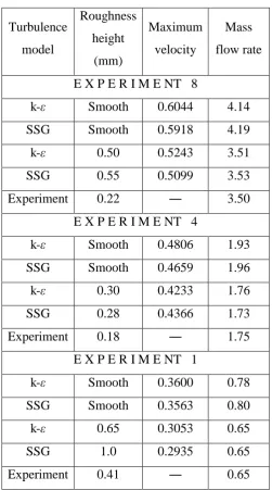
in coastal zones with oscillatory waves. One detailed estuarine study is described by Knight

(Knight 1981), who measured the relative importance of the various terms in the 1-D St

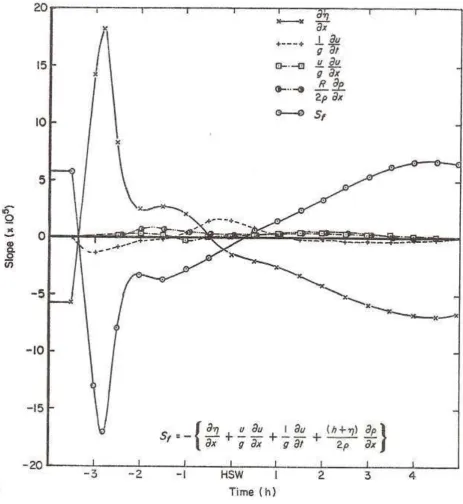
Venant equation through many tidal cycles on the Conwy estuary. Figure 1 shows some

results, and Figure 2 shows how the resistance to flow is ebb-dominated as the sand dunes

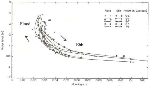
respond to the longer period of ebb flow. Figure 3 shows that for this particular tidal reach,

the ks values at low tide (ks ~ 8 m when h ~ 1 m) are very much greater than at high tide (ks ~

0.2 m when h ~ 6 m), and indeed even greater than the depth of flow. Although surprising,

this feature is not inconsistent with the meaning of ks and the way in which it varies with the height of an individual roughness element, k, in this case the sand dunes on the estuary bed.

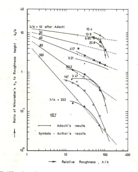
On a different, but related topic, Figure 4 shows that for a regular rib-type of roughness, the

value of effective roughness height to actual height of the roughness varies considerably (10 >

ks/k > 0.01), and depends on at least two other parameters, h/k and /k, where is the longitudinal spacing of the roughness elements. The friction factors for many other types of

rib-roughness are documented in an Engineering Sciences Data Unit report (ESDU 1979), on

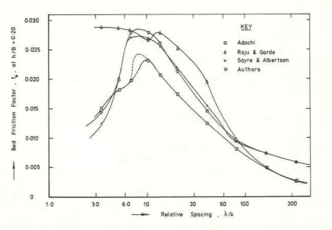
account of their use in heat transfer calculations. In general it is known that resistance will

peak when the /k value is between 8 and 12, as shown by the data for square rib elements in

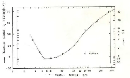
Figure 5. For these types of roughness it is more appropriate to use a factor, , which then

produces a logarithmic variation with U/U_*, (Sayre & Albertson, 1963) governed by

      

 h U

U

ln 06 . 6

*

(1)

as shown in Figure 6, provided it is specified as shown in Figure 7. The use of should be

seen as a surrogate or alternative for ks. Further details are available elsewhere (Knight and

Macdonald 1979). The unusually large ks value may lead to conceptual difficulties in 1-D

if one links ks and k directly. These studies also show the importance of recognising that there

are other key ‘characteristic’ dimensions for roughness other than the single value of a

roughness ‘height’, ks, usually considered as being normal to the mean position of the

boundary surface. The actual mean position of the surface (i.e. datum plane) is particularly

important when considering sediment beds with dunes (1984), rivers with variable topography

(Nicholas, 2001) or rib-type roughness (Macdonald, 1976).

Unsteadiness in the flow is known to alter the turbulence structure (Song and Graf 1996) and

consequently bed shear and resistance. An important study of the impact of unsteadiness in

flood analysis is shown by Sellin & van Beesten (Sellin and van Beesten 2004) who

monitored the floodplain resistance on the River Blackwater. Figure 8 shows the typical

looped nature of floodplain resistance. Flattening of vegetation may produce a clockwise

sense of rotation in the loop rather than the customary anticlockwise one associated with the

1D convective and local acceleration terms. Laboratory studies in unsteady flow by Graf &

Qu (Graf and Qu 2004) and Lai et al. (Lai et al. 2000) not only confirm the looped nature of

resistance but also some problems of defining a bed friction factor. For periodic flows, a

review of how boundary shear is affected by oscillatory boundary layer effects is given by

Knight (Knight 1978). This has implications not only for near bed dynamics in coastal zones,

but also in small scale physical models of estuaries where oscillatory boundary effects are

enhanced (Knight and Ridgway 1976, 1977; Sleath 1984).

Vegetation within or alongside a river channel also greatly affects the resistance to flow.

Seasonal growth and decay, as well as managed weed cutting programmes, mean that

instream and bankside vegetation typically vary spatially and temporally within most

managed river systems. General guidance about the effects of vegetation on resistance is

given elsewhere (Kouwen and Unny 1973; Klaassen and van der Zwaard 1974; Kouwen and

Li 1980; Kouwen et al. 1980; Hasegawa et al. 1999; Yen 2002; Dawson and Fisher 2004;

Jarvela et al. 2006). The vegetation on floodplains may be of a more varied and dense nature

and may require special treatment (Ikeda et al. 1992; Centre 1994; Ikeda et al. 1999). The

effect of vegetation on flow structure in compound channels has been described by Okada &

Fukuoka (Okada and Fukuoka 2002, 2003).

from resistance due to the textural roughness of the plane surface, and that due to form

roughness arising from separation and vortex shedding on the downstream side of bed forms.

The total resistance is then considered to be the sum of the two components. Since the

geometry of bed forms change with velocity and depth of flow, alluvial resistance

relationships are much more complex than those of rigid boundary channels (e.g. f v Re for

different ks/4R values, as in the Moody diagram or Colebrook-White equation (Myers et al.

1999; Knight and Brown 2001).

Assuming that the resistance of an alluvial channel may be conceptualised in this way, then

either the energy gradient, Sf, or the hydraulic radius, R, may be considered to be divisible

into two elements. Thus, the energy slope may be written as

' ''

S S S (2)

where S' is the slope of the energy line due to grain resistance on a plane bed, and S'' is the

additional slope due to the bed forms. Using the Darcy-Weisbach law for S gives

2 ' 2 '' 2

8 8 8

fU f U f U

gR  gR  gR (3)

 ' ''

f  f  f (4)

where f' and f'' are the friction factor counterparts to S' and S''. Alternatively by considering

the hydraulic radius, R, to be divisible into two components, then

' ''

RRR (5)

where R' is the component associated with grain resistance and R'' is that associated with form

resistance. Multiplying Equation (5) by _{gSf gives}

' ''

f f f

gRS gR S gR S

 ' ''

o o o

   (7)

where _{o' is the boundary shear stress associated with grain resistance and} _{o'' is the boundary}

shear stress associated with form resistance. It should be remembered here that _{o is a}

‘global’ 1D value, and that the distribution of ‘local’ boundary shear stress around the wetted

perimeter of an open channel is governed by the shape of the cross section, the number and

pattern of secondary flow cells and other considerations (Knight et al. 1994).

The values of R' and S' may be determined from traditional plane bed rigid boundary

resistance laws, such as the Colebrook-White equation or its corresponding graphical form,

the Moody diagram. Eqs (4) & (7) indicate that f' and _{o' are counterparts to S' whereas f'' and}

_{o'' are counterparts to S''. The main difficulty encountered in sediment resistance studies is}

in determining suitable relationships for f'' (of its corresponding Manning value, n'') for

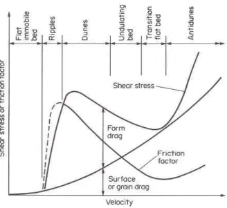
different flow and sediment conditions. The general form of the resistance relationship for an

alluvial channel is shown in Figure 9. Below threshold the resistance typically decreases as

the Reynolds number (or velocity) increases. Once threshold has been passed, the resistance

increases rapidly by a factor of 3 or 4 as ripples and dunes are formed, reaching a maximum

before decreasing again as the dunes are washed out as transitional flow is reached. The

resistance thus peaks in the lower flow regime, reaches a minimum in transitional flow and

then increases again in the upper flow regime. The details of this relationship are described in

many specialist texts (Raudkivi 1967; Garde and Ranga-Raju 1977; van Rijn 1984; Chang

1988; Yen 1991; Simons and Senturk 1992; Yalin and Ferreira da Silva 2001). An example

of how the bed forms affect resistance is shown for the River Padma, Pakistan, by Shen (Shen

1971). The latter also highlights the subtle effect of water temperature on flow resistance, a

feature often ignored, using data from the Mississippi River.

A final consideration in roughness studies involving 1-D modelling, and to a certain extent in

2-D modelling, is the issue of how the longitudinal energy gradient, Sf, should be averaged

over a channel reach. This is discussed by Laurenson (1986), and is of significant practical

interest. Guidance on how heterogeneous roughness may be obtained from disparate inputs is

also of significance, and further details are available in the Roughness Advisor (RA),

3 Roughness characterised by a roughness height

3.1 General approaches

Despite the difficulties outlined above and in the absence of any alternative, many engineers

still feel the need to characterise fluvial roughness by a specific roughness or resistance

‘height’. This is especially true when they deal with rigid planar surfaces. Indeed, many

researchers have erroneously attempted to investigate the physical meaning of this parameter,

simply because it makes some sense from an experimental or practical standpoint. Because of

the vast types of roughness in rivers, this paper will concentrate on planar surfaces and not

consider resistance from either sedimentary bedforms or vegetation. Quantification of these

different effects remains difficult as evidenced by the widespread range of formulations

available in the literature (Yen 1991). As a result, with the current available knowledge,

roughness height mostly remains a calibration parameter, used to tune numerical model

outputs to measured data. Its meaning is however unsure. Because of its continued use, it

will be explored briefly now, prior to considering in detail how roughness should be

formulated in 1-D, 2-D & 3-D models.

3.2 Roughness Height and Roughness Value

Historically, the relationship between roughness and particle diameters was investigated in

relatively smooth experimental channels to quantify the roughness height, ks, on the grounds

that the most obvious form of roughness was that created by grain irregularities at the wall.

Clearly this approach limits the use of ks and its widespread application in numerical models. Nevertheless, this type of relationship has remained and has been implemented in much

practical research, relating roughness height to particle size in channels.

Several formulations such as ks 3.5D84 or ks 6.8D50, where DXX stands for the grain

diameter for which xx% of the particles are finer, have been given as reported in Clifford et

al. (1992). Unfortunately, the nature of the momentum loss mechanism included in such

formulae is not really well known; the level of theoretical detail considered in the formulation

of the problem, in order to link both roughness height and grain diameter, and the flow

characteristics are often not tied to the equation when it is subsequently used which is

particles (D50 = 40 mm), which resulted in the calculation of different coefficients, e.g. quite logically for grain roughness, k_g 0.30.5D₅₀ (skin friction). The use of Clifford’s results

shows that the grain-roughness relationship is inadequate for determining the overall

roughness height, as grain-related roughness seems to cause low momentum losses. Formulae

such as k_s 6.8D₅₀ therefore include several momentum loss mechanisms that are not well

understood, nor quantified, resulting in inappropriate roughness height values when different

grains or different flow conditions are modelled.

There is still uncertainty regarding the relevance of the above formulae outside the range of

conditions for which they have been derived. Most of the work that has led to the above

formulations has been done for limited ranges of particle diameters. For example, Whiting &

Dittrich (1990) reported a range of values between 0.68 and 7.7 mm and seem to include all

roughness effects shown previously, while Clifford et al. (Clifford et al. 1992) used a mean

diameter in the region of 40 mm. Formulae such as ks 6.8D50 or ks 3.5D84 seem to

have been derived for relatively small grains, yet are now applied beyond these ranges by

some Computational Fluid Dynamics users without being questioned. In some cases this has

lead to values of ks being as large as 0.250 m (Nicholas and Walling 1997; Hodskinson and

Ferguson 1998). This is quite problematic on both numerical and physical grounds: in such

cases the cell next to the wall should be larger than the value of ks which requires large cells

that reduce accuracy. Therefore the roughness value cannot be chosen independently of

numerical and physical considerations relevant. The fundamental problem is using a

roughness model based on theory from sand-grain roughness for roughness elements that are

considerably larger.

Finally, although not considered here, it should again be emphasised that use of a single

parameter such as ‘roughness height’ will be inadequate wherever other spatial scales exist,

such as in periodically spaced roughness, where the wavelength, , is important (e.g. rib

roughness or earlier discussions on sediment and bed forms). Similarly when vegetation is

present and becomes submerged, a horizontal shear layer form will form in the surface flow

region above the canopy and penetrate to some depth within the plants, giving rise to unusual

4 Roughness in the 1D, 2-D and 3-D transport equations

As mentioned in the introduction, roughness does not appear explicitly in the 3-D

Navier-Stokes equations. Roughness is introduced at the walls to account for small momentum and

energy losses that are not embedded in the discrete formulation of the continuous problem.

Roughness also appears in the St Venant form of the Navier-Stokes equations in 2-D and 1-D,

usually accompanied by a decreasing level of accuracy in terms of the physics embedded in

the model, e.g. turbulence and the effect of geometry. The following sections discuss the

meaning of roughness for these various models.

4.1 Roughness in 1-D models

From the previous comments, it is clearly difficult for a modeller to attribute a roughness

height to a given channel. Hydraulicians often prefer to use a Manning’s n roughness

coefficient when it comes to open channel friction losses as it is often (mistakenly) regarded

as less flow dependent. All such “lumped” parameters, including the Colebrook-White

friction factor, f, and Chézy’s C, are subjective to determine and are dependent on the channel

geometry and flow characteristics (levels). Additionally the level of detail encompassed in

the model also affects the meaning of these parameters. A typical example is whether the

description encompasses turbulence effects or not. In a 1-D representation the roughness

model does encompass turbulence, but in some 2-D models it does not: therefore, a 2-D

model should not necessarily use the friction factor from a 1-D model

General formulae have been proposed to relate particle diameters to Manning’s n values and

the latter to equivalent roughness height. One is derived from the HR Wallingford tables

(Ackers 1958) and yields:





038 . 0 / ) (mm n

k_s  (8)

This only applies for a limited range of ks where the condition10 R/ks 100 (R = hydraulic

radius) is satisfied, which confirms application to rough engineered canals and natural

A more general approach is therefore needed. Massey (Massey 1995) gives a theoretically

derived equivalence in his textbook

         n R R SI k_s 6 / 1 10 0564 . 0 exp / 86 . 14 )

( . (9)

(9) is quite close to the derivation in Chow (1959)

         n R R SI ks 6 / 1 10 0457 . 0 exp / 20 . 12 ) ( (10)

From (10) Strickler (1923) arrived at an average:





0342 . 0 / ) (ft n

k_s  (11)

assuming a median grain-size. As reported in Chow (1959), Equation (10) was successfully

applied in the United States, and in particular on the Mississippi. Krishnappan and Lau

(1986) also used (11) for their three-dimensional model of floodplain flow.

For the FCF experiment (Knight and Sellin 1987) however an equation such as (8) yields an

improbably small value of the order of a fraction of a micrometer. When R /ks is calculated

for this experiment, it appears that it is 3 to 4 orders of magnitude larger than the upper limit.

Consequently equations (9) to (10) are used and yield values in the range 2.0104to

4

10 0 .

8   m, which seems to fit reasonably well with the table given in French (French 1985)

for simple, smooth materials or surfaces. However, as underlined in Chow (Chow 1959), the

above formulae were usually used to evaluate Manning’s n values from values of ks, for

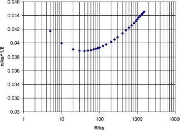
which the resulting n is relatively insensitive, see Figure 10, based on Equation (12), in the

range 10 R k_s 100 and Yen (1992). The converse is not true and leads to large ranges of

roughness height values for small variations of Manning’s n, especially when n is large, see

Figure 11.        ) / 11 log( 18 ) / ( 1/6

For the purposes of channel resistance, the mean boundary shear stress is also traditionally

linked to the section-mean velocity, U_A, by the ‘global’ or overall friction factor, f, by the

empirical, yet dimensionally valid, relationship given by the first part of equation (19).

The resistance relationship for flow in smooth and rough pipes of circular cross-section is

usually given by the Colebrook-White equation:

           f UR R k f s ) / 4 ( 51 . 2 8 . 14 log 0 . 2 1 10  (13)

where U = Q/A, R = d/4, d = pipe diameter, and k_s = Nikuradse equivalent roughness size.

Such a relationship assumes a logarithmic velocity distribution within the boundary layer that

applies over the bulk of the cross-section. In a river, it is often assumed that the vertical

distribution of the streamwise velocity distribution may be approximated by that in a

boundary layer on a flat plate in rough turbulent flow. Near the bed the steep velocity

gradient is indicative of large shear stresses, considered as turbulent Reynolds stresses applied

internally on the fluid by the action of the flowing liquid. Assuming a rough turbulent flow,

then the local velocity, u, distance z above the bed is given by

       s k z U U 30 log 75 . 5 * (14)

where the customary ‘rough turbulent’ coefficient of 8.5 in the standard ‘rough’ law for f has

been subsumed into the log term. Since the depth mean velocity occurs at 0.37depth,

Equation (14) becomes

       s d k h U U 11 log 75 . 5 * (15)

where h is the depth of flow. The value of ks may be related to the mean grain size, D₅₀, as

If the Manning equation is adopted instead of the Darcy-Weisbach equation, then the link

between Manning’s n and ks may be given by Equation 12. It should however be remembered

that the use of simple logarithmic velocity relationships should be carried out advisedly, given

alternative analyses and the definitions of boundary shear stress (Prokrajac et al. , 2006;

Nikora et al. 2004; Olsen & Stokseth 1995).

4.1.1 Roughness in quasi-2-D models

For straight prismatic channels, the streamwise depth-averaged RANS equation is given by

Knight and Shiono (Knight and Shiono 1996) as









d d

d d

o H UV

y y U U f H y s fU gHS                                   2 / 1 2 2 / 1 2 2 8 1 8 1

1 (16)

where s = transverse side slope of channel (1:s, vertical: horizontal) and = dimensionless

eddy viscosity (  yxU_d /y and yx U_*H). Equation (16) may be written as

  





   

  _o yx

b H

y gHS

s  

 

 1 1₂ 1/2 (17)

where it is assumed that the boundary shear stress, _b, is related to the depth-mean velocity,

U_d, by a local friction factor, f, the turbulence is simulated by an eddy viscosity approach, and

 is the right hand side of Equation (17).

When using resistance coefficients in these models, care then needs to be taken to distinguish

between ‘global’, ‘zonal’ and ‘local’ friction factors, based on using the section-mean

velocity, U_A, the zonal velocity U_z, or the depth-mean velocity, U_d, respectively. In the latter

case, U_d is used technically to replace the law of the wall approach in 3-D models, in that it

relates boundary shear with a ‘local’ velocity. Thus by analogy with the 1-D Darcy-Weisbach

equation, it follows that:

2 8 A o U f _       

 2

Equation (18) indicates that the boundary shear stress, _b, is influenced by the lateral shear

and secondary flow and may differ significantly from the value based on local depth (_b 

gHSf), as mentioned previously. Unlike 1-D methods, which have just one lumped parameter,

such as f or n, in the Shiono & Knight Method (SKM) there are now three calibration

coefficients, f,  and , concerned with bed friction, lateral shear (via depth-averaged eddy

viscosity) and secondary flow (via lateral gradient of H(UV)_d) respectively. There is now

therefore the possibility of simulating the lateral variations of U_d, _b, yx and  within the

river channel. A numerical or analytical solution to Equation (16) may be obtained by

discretising the cross-section boundary into a number of linear elements, and specifying the

three coefficients, f, , and , for each sub-area. Further details can be found elsewhere

(Knight and Abril 1996; Abril and Knight 2004).

Analysis shows that the relative contributions of the depth-averaged Reynolds stress term, _{yx, and the secondary flow term, (}UV)_d, to the apparent shear stress (ASS) are known to be

roughly comparable in magnitude (Knight and Shiono 1990; Shiono and Knight 1991),

highlighting the importance of vortex structures in resistance studies. Numerical work by

Thomas & Williams (1995), using data from test series 22 from the FCF and a large eddy

simulation (LES), confirms this finding.

The stage-discharge relationships in most 1-D commercial software packages for river

engineering are typically based on one of the 1-D ‘divided channel’ methods (DCM),

described elsewhere (Knight 2005). These methods all assume quasi-straight river reaches,

and since they do not include any lateral momentum transfer effects, they are inevitably not

particularly suitable for predicting accurately either the water level in compound river

channels or the proportion of flow that occurs on the floodplains. More recent 1-D river

engineering software (www.river-conveyance.net) will include the effect of flow structure,

through the adoption of improved methods (Knight, 2005). These may be grouped under the

headings: the ‘divided channel method’ (DCM), the coherence method (COHM), the Shiono

& Knight method (SKM), and the ‘lateral division method’ (LDM). Several authors have

4.2 Roughness in 2-D models

4.2.1 Friction representation in 2-D Shallow Water models

The 2-D Shallow Water equations can be derived by physcial arguments similar to those used

in 1-D or by vertical integration of the Navier-Stokes equations. Friction is parameterised in a

similar way to 1-D through, for example, Manning’s n or Chezy’s C. The appropriate

equations are (Nezu and Nakagawa 1993):

2-D mass conservation:

l Q y hv x hu t h _         (19)

2-D momentum conservation:

) ( 2 fx ox S S gh x h gh y huv x hu t

hu _{ }

           (20) ) ( 2 fy oy S S gh y h gh y hv x huv t

hv _{ }

           (21) where 3 7 2 2 2 h v u u n

S_fx  or

h C v u u S_fx 2 2 2 

 and

3 7 2 2 2 h v u v n

S_fy   or

h C v u v S_fy 2 2 2  

Other terms can be included to represent the effects of turbulence, although this is often left to

the friction term. The determination of n is not straightforward and this raises a number of

issues that are similar to those discussed earlier in the context of 1D modelling (

www.river-conveyance.net). Therefore they are not addressed here.

As mentioned briefly before, even though 1-D and 2-D representations use Manning’s or

Chezy’s coefficient, the roughness model is different. The 1-D representation is using the friction factor to represent the shear stress exerted by the entire bed and banks bounding the

flow whilst a 2-D model is using the factor to represent the shear stress exerted at the base of

a vertical column of water: these are not the same situation. Additionally, the 1-D

representation does not take explicit account of the effects of turbulence in removing energy

turbulence models are sometimes explicitly included through terms in addition to the friction

term and in these cases the friction factor will differ.

4.3 Roughness in 3-D models

The term 3-D model is taken here to mean models that solve the Navier-Stokes equations in

all three dimensions. In such models a no-slip condition usually applies at the walls, which

means that the velocities tangential and normal to the walls are zero. Close to the walls, the

Navier-Stokes equations would require a very fine grid to properly resolve the linear

sub-layer and the turbulent boundary sub-layer. This requirement is removed by replacing the grid by

a model of the boundary layer in 3-D models, i.e. the wall function. This function allows for

the computation of the wall effect at the first node inside the domain.

In the vicinity of the wall it is assumed that the fluid shear stress is equal to the wall shear

stress, _t





sub-layer of the boundary layer, the velocity distribution is given by:



 y u u

*



(22)

where u_ is the tangential velocity, parallel to the wall, u_* is the shear velocity, and



*

yu

y  is the non-dimensional distance normal to the wall. The transition between

laminar and turbulent flow regions has been determined experimentally to be between y 5

to 30 (buffer layer), with various transition velocity laws proposed (Reynolds 1974). In order

to simplify boundary layer analysis, it is sometimes assumed that the transition occurs at the

position where the laminar and turbulent laws distribution laws meet, i.e. at y 11.63

(Chang 1988).

In the turbulent shear flow region a general form for the law of the wall can be given as:

) ) ( ln( 1

*

  _

 E k y

u u

s



 ₍₂₃₎

where, E(k_s) is a function of the non-dimensional roughness height, k_s k_su_* , in which

ks is the roughness height, is von Karman’s constant usually taken equal to 0.41 and is the

i) Hydraulically smooth: 0 . 9 ) ( 5 . 5 ) ln( 1 *        E k E y u u s  

ii) Transition:





 s s s s

s k g k E k g y k f k y u u    

iii) Hydraulically rough:

        s s s k k E k y u u 30 ) ( 5 . 8 ) ln( 1 *  

where y is the non-dimensional distance from the wall. However, a function needs to be

formulated for E(k_s) in the transition condition.

In most CFD codes, the hard-coded formula for the law of the wall is valid for smooth

surfaces. A function that will extend the validity of the law of the wall beyond smooth

surface boundary conditions and/or low turbulence models is consequently required. This is

not difficult for a hydraulically rough surface as the function is clearly defined by the theory

(see (iii) above), and it has been successfully implemented in Launder and Spalding (1974)

for example. However, a general function for E(k_s), which covers the whole range of

boundary conditions while remaining sufficiently robust needs to be formulated so that it can

cover the entire range of k values independently and more flexibly. _s

The difficulty lies in formulating a function g(k_s) that is continuous and tends

asymptotically towards 9.0 for small k values and towards _s 30 k_s when k becomes larger _s

than 70. Mathematically a simple first assumption could consequently be looking at a

function of the type  _    s s k c b a k

g( ) , with 9.0 b a

and 30.0 c

a

. The simplest function of

this kind is:

Because of the function properties, one can generalise the above proposal to give:        s s s k E k E , k 3 . 0 1 ) ( (25)

The above function is very close to a proposal made by Naot (Naot 1984), who gave:

                          s s s k k E k E 20 1 3 . 0 1 )

( (26)

A similar approach is adopted in the commercial codes (i.e. FLUENT and CFX) under the

general form  _    s s k c E k E 1 )

( (c = constant).

Other approaches consider the experimental work of Nikuradse (Nikuradse 1933) on

roughness, and use the experimental results to fit a function to his data points. Three other

approaches are by Cebeci and Bradshaw (1977), Yalin (1992) and Sajjadi and Aldridge

(1993). These are relatively complex which may not make them suitable as a robust

all-purpose model.

Whichever formula is applied, attention should also be paid to the position of the first node on

the grid, close to the wall. A near wall flow is taken to be laminar if y 11.63. It is

therefore important to ensure that the finite element grid does not encroach into this region,

otherwise a transport equation validated for turbulent region will be applied in a region of

laminar flow and a significant error will occur. Modern solvers have this facility built in and

are able to move the node “algebraically” in order to allow for a suitable implementation of

the law. In flows with recirculation at the wall, the velocity component parallel to the wall at

the re-attachment point is zero, which means that the simulation reverts to the laminar case

(Versteeg and Malalasekera 1995), which further demonstrates the difficulty of this approach.

flow velocity profiles. Despite increasing computer power this is not always achievable when

modelling large-scale geometries and this should be taken into account during the discussion

of the results. With the ever increasing computer power available to modellers, this is

becoming less of an issue.

The law of the wall is then incorporated into the model equations via an extra shear term that

mimics the effect of the wall on the fluid at the first node off the wall. The law of the wall

therefore allows the physical effect of the wall boundary to be reflected into the discrete

domain, where the discretised Navier-Stokes equations are solved.

As an alternative to the law of the wall approach to modelling roughness the effects of

vegetation and large boulders at a boundary are sometimes modelled using a ‘porosity’ approach. These porosity terms enable the computation of an ‘equivalent’ momentum loss

added to the Navier-Stokes equation where a large obstruction is present and Lane (Lane et al.

2005) has recently suggested this approach as a suitable alternative.

5 Discussion

Whichever resistance coefficient (f, n or k_s) is used, its origin and basis should be understood,

and its numerical value properly assigned in order to obtain the correct boundary shear stress

from calculated or measured velocities. It should also be noted that the sub-area and

depth-averaged friction factors defined in Equation (18) implicitly include the effects of secondary

flow, vorticity and lateral shear. This also implies that appropriate f,  and  values must be

specified in SKM if lateral distributions of both U_d and _{o are to be determined accurately.}

Likewise, k_s values need to be specified carefully in 2-D and 3-D numerical models.

Whatever resistance coefficient is used, it should always be remembered that resistance values

are usually strongly depth, and hence flow, dependent (ASCE 1963; Knight 1981; Wallis and

Knight 1984; Knight et al. 1989; Hicks and Mason 1998; Dawson and Fisher 2004).

It is sometimes convenient to use a 'composite' roughness coefficient for the whole channel,

based on aggregating values from individual sub-areas, rather than many individual values.

geometry have been highlighted, there are occasionally problems where it is convenient to

adopt this approach. See Yen (Yen 1991; Yen 2002) for further details.

5.1 Should calibration use the roughness coefficient or friction factor?

The practice in experimental work and St Venant based modelling is to characterise the wall

surface in order to select an appropriate friction coefficient and to adjust the model outputs

via this parameter. This is understandable since the roughness coefficients appear explicitly

in the equations and can have a significant effect on solutions. For example, using Chezy’s

model for roughness in the 1D momentum equation:





sin ₍₂₇₎

It is clear that the impact of the roughness factor (viz. roughness term or energy loss term Sf)

on these equations is significant, especially as the “channel” gets “rougher”, as can be seen in

Figure 12, where Sf varies exponentially with increased roughness. For a given surface slope

the level of uncertainty in the choice of the roughness value and the relationship between

roughness and discharge are very clear. The energy loss term is just one amongst the local

acceleration term, convection term and head and gravity forces. The magnitude of the term

on the right hand side has significant consequences for the numerical convergence and

therefore as part of the iterative solution process it is usually preferable to have small forcing

terms such as g(S_o S_f) in the previous equation.

On the other hand roughness is a much smaller term when solving the full 3-D Navier Stokes

equations. Roughness appears in the boundary condition rather than as a term in the

equations (as in 1-D and 2-D). The impact roughness has on the solution is therefore much

more localised and limited. Thus, it is clear that in different dimensional representations in

open channel flow, the role and impact of the roughness value upon the solution are very

different and this value does not represent the same physical effect. This is illustrated in

Figure 13 which shows numerical results based on Kenneth Yuen’s Experiment 16 (Yuen

seen that the 1-D results are significantly more sensitive to changes in the roughness

parameter than the 3-D simulation. It is clear that the role of roughness in terms of calibration

is more limited in higher dimensions. Other effects have to be considered in addition to

roughness. As a consequence, it must be said that roughness cannot compensate for errors in

the numerical technique or the physical model. Therefore calibration based on roughness

values should be limited in its scope and it should be ensured that roughness values remain

within physically appropriate limits.

It is difficult to define the roughness of one region generically without consideration of the

flow characteristics, physical models and level of numerical discretisation used in the

simulation. This makes the process of model calibration very uncertain and the

“establishment” of one roughness value impossible. The authors’ experience combining experimental with numerical work shows that if the “physical” roughness value is adjusted to

ensure the correct value for the free surface position, discharge and slope, then an equivalent

numerical roughness value can be calculated. The exact values of this depends on the

turbulence model and numerical characteristics of the simulation, and is usually different

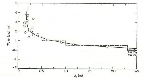
from the experimental value. In recent work for simple channels (Wright et al. 2004; Morvan

et al. 2005) the mass flow and bed shear stress values, known from the experiments and the

theory, were used as objective functions to adjust the roughness values. In most cases the

roughness values necessary were different between k- and Reynolds Stress Models, typically

by about 10% but, on occasions, by as much as 50%. This is shown in Table 1 based on a

number of simulations (Wright et al. 2004) of experiments carried out by Yuen at the

University of Birmingham (Yuen 1989; www.flowdata.bham.ac.uk). Clearly these values do

not match with experimental data which are given in the tables based on Manning’s equation

and Equation (12), although their variation is consistent with the CFD values. This is not

inconsistent as the different values are representing different models: the physical one

typically represents a bulk value based on bulk shear stress and the numerical one in 2-D and

Turbulence

model

Roughness

height

(mm)

Maximum

velocity

Mass

flow rate

E X P E R I M E NT 8

k- Smooth 0.6044 4.14

SSG Smooth 0.5918 4.19

k- 0.50 0.5243 3.51

SSG 0.55 0.5099 3.53

Experiment 0.22 3.50

E X P E R I M E NT 4

k- Smooth 0.4806 1.93

SSG Smooth 0.4659 1.96

k- 0.30 0.4233 1.76

SSG 0.28 0.4366 1.73

Experiment 0.18 1.75

E X P E R I M E NT 1

k- Smooth 0.3600 0.78

SSG Smooth 0.3563 0.80

k- 0.65 0.3053 0.65

SSG 1.0 0.2935 0.65

Experiment 0.41 0.65

Table 1. Summary of results for trapezoidal Experiment 8, 4 and 1 (Yuen, 1989). Experiment roughness values are back calculated from the mass flow rate value, using

Manning’s equation and equation (12). SSG is the Reynolds stress turbulence model by

Sarkar, Speziale and Gatski (1991).

The above leads to the conclusion that, in 3-D, roughness is a calibration parameter in a

somewhat similar, but less significant, way to simpler 1-D models. The main difference for

roughness and roughness values is in the amount of physics that each level of flow model

encompasses (lateral and vertical velocity, density, turbulence) and this leads to roughness

having a quite different meaning at each dimensional resolution. The points raised in this

roughness. On the subject of scales, the paper has raised another issue of interest: roughness

does not have the same measure in all models or model substantiation. A 1D modeller or an

experimentalist will talk about the reach or flume roughness, whilst a 3-D modeller will talk

about skin roughness with the other components being embedded in the geometry, turbulence

and particle models for example. This argument can be illustrated by the approach that a river

modeller would take compared to a CFD modeller: the former would usually adjust roughness

to improve model results whilst the latter would not think to do this until they had examined

the mesh quality, discretisation and turbulence modelling.

What we cannot systematically represent mathematically or physically we cannot really

“measure” and therefore one thing we know is that proposals for constitutive laws linking

roughness to particle diameter, for example, are misguided – especially without the bounds of

the assumptions for which the equation was established. Furthermore roughness is implicit: it

is a function of the flow it governs, as the reach roughness depends on the water depth and

low speed in the river for example. It is not a function of the grain size only, as many may

have forgotten in the wake of Nikuradse’s particular experiments. This is just the same as

with eddy viscosity: whilst viscosity is a fluid property, eddy viscosity is a property of the

flow. One has to accept that roughness is still a calibration parameter in computational

models, especially when we model natural geometries where the insights that we have gained

in an idealised laboratory channel do not always apply. This does not make things easy for

practitioners. However, trying to correlate field data with a unique ks value is potentially

dangerous without a warning message attached to the formula.

Consequently it is quite legitimate to find that there exist several roughness values for the

same model: one experimental, that can be used as an initial guess in the CFD model, and

some numerical ones, functions of the other models and the updates that the educated user

makes.

5.2 Use of roughness to represent large features

Traditionally and following Nikuradse’s pioneering work researchers have attempted to relate

particle size to roughness height. This has been proved to work for small size particles such as

numerical modelling, without questioning their validity and the size of the sink term they

represented and comparing it to the sink term necessary to truly balance the equations. In the

context of numerical models, additional numerical considerations are indeed necessary to

make sure this approach satisfies the equation balance but also, and equally importantly, to

ensure that the roughness parameter is consistent with its physical interpretation in terms of

size relative to the grid size and therefore in relation to the obstruction to fluid movement

within the cell. Increasing the size of the roughness parameters has serious impact on the

algebraic equations as illustrated in Figures 12 and 13. These considerations are sometimes

ignored by modellers.

The authors believe that this approach is flawed for any particle that is large relative to the

problem size. A lot of the approaches attempting to relate particle size and roughness rely on

a simple logarithmic profile to build the equivalence and are often found to be river or reach

dependent, which indicates that the approach probably does not consider all the necessary

parameters but, more importantly it is likely not to be the correct approach. This is, again,

made worse when trying to apply the same approach to models 1-D, 2-D and 3-D for which

roughness has a different meaning. In the context of numerical modelling the authors would

favour solely numerical considerations in setting up a model with subsequent comparison

with measurable physical values such as shear stress, etc.. A roughness model should be a

sink term, the suitability of which could be measured in terms of equation balance

considerations and water level slope in hydraulics. It is also clear that more work is required

to understand fluid behaviour at the walls. The authors are actively investigating quadratic

porosity models based on Darcy’s equation. The factors for these are derived using models of

flow around the kind of dowels used in experiments.

5.3 Roughness and modelling in engineering practice

This issue is crucial in 1-D river modelling where practitioners seek a conveyance coefficient

2 1

/S_f Q

K which often relies on a “roughness” value associated to a list of physical

characteristics such as particle size(s) and vegetation type. Unfortunately such a definition,

already difficult conceptually, is made even more complex as the model dimension decreases

because the roughness factor accounts for more physical phenomena such as turbulence,

particularly in 1-D. Of course it must be recognised that in 1-D the real issue is to determine

some hope to a practitioners dilemma through the development of approaches such as the

Conveyance Estimation System (www.river-conveyance.net) by HR Wallingford for the

Environment Agency which is helpful in moving the focus from the uncertainties of

estimating friction factors to conveyance estimation and also implementing state-of-the-art

methods for estimating conveyance such as the SKM mentioned above.

When moving from 1-D to 2-D matters are not much easier despite the possible introduction

of turbulence modelling. In 3-D the identification of what roughness stands for is made easier

because more physics is included; yet, the definition of the “roughness height” is also very

limited by the lack of fundamental understanding of what roughness is and the lack of a

generic law describing its effects.

6 Conclusions

It is clear that modelling open-channel flows is not straightforward and needs the combined

expertise of experimentalists and numerical modellers. On the basis of experience in both

these fields, the authors have drawn a number of conclusions:

 Roughness varies between models which represent different dimensions. Consequent

on this, it must be recognised that reach-scale roughness is a different concept from

local roughness.

 Using roughness to represent features other than sand-grain roughness lessens the

validity of the underlying theory and is questionable.

 Models of roughness in 1-D hydraulic models are valid and will continue to be useful when based on CES and calibrated appropriately. Conveyance estimation can ensure

that the latest results from experimental work and complex numerical modelling are

transferred into practice.

 1-D modellers should focus more on estimating conveyance than establishing one sole

value of Manning’s n or Chezy C for a channel.

These arguments indicate that even the modelling of idealised laboratory channels is not

straightforward and therefore the modelling of real rivers is an even more complex task.

there is significant benefit of using hydraulic models compared with say, hydrological

models, but it is hoped that this paper has demonstrated that care must be taken in their

application.

This paper is clearly part of an ongoing discussion on these issues. The authors hope that

List of Symbols

a = constant

A = cross-sectional area

b = constant

c = constant

C = Chézy C

d = diameter

Dxx = grain diameter for which xx% of the particles are finer

f = friction factor _

       gR U f gR U f gR fU 8 '' 8 ' 8 2 2 2

f ‘= friction factor (associated with grain resistance)

f ‘’= friction factor (associated with bed forms)

g = acceleration of gravity

h = flow depth

ks = Nikuradse equivalent sand roughness

ks+ = non dimensional equivalent sand roughness        _ * u k k_s s

k = roughness height

K = conveyance coefficient _      

 _1/2

f

S Q K

n = Manning’s n

P = wetted perimeter

Q = mass flow

R = hydraulic radius        P A R

Re = Reynolds number       _  Ud Re

s = transverse side slope

S = energy slope





S’ = slope of the energy line due to grain resistance on a plane bed

S’’ = additional slope due to the bed forms

UA = area mean velocity Ud = depth mean velocity Uz = local/zonal velocity

V = transverse velocity

u = tangential velocity u* = shear velocity

v = velocity along the y-axis

y+ = non dimensional distance from the wall z = a distance (e.g. from the wall)

= longitudinal spacing of roughness elements; dimensionless eddy viscosity = kinematic viscosity

b = boundary shear stress (depth averaged, function of Ud) o = boundary shear stress (global value, function of UA)

o’ = boundary shear stress associated with grain resistance

o’’ = boundary shear stress associated with form resistance

References

Abril, J. B. and D. W. Knight (2004). "Stage-discharge prediction for rivers in flood applying a depth-averaged model." Journal of Hydraulic Research 42(6): 616-629.

Ackers, P. (1958). Hydraulics Research Paper: Resistance of fluids flowing in channels and ducts, HMSO. 1: 1-39.

ASCE (1963). "Friction factors in open channels [Task Force on Friction Factors in Open Channels], Journal of the Hydraulics Division, Proc. ASCE, Vol 89, HY2, March, 97-143 (Discussion in Journal of the Hydraulics Division, Vol 89, July, Sept. & Nov., 1963 and closure in Vol. 90, HY4 July 1964)." Journal of the Hydraulics Division Proc. ASCE, Vol 89, HY2: 97-143.

Cebeci, T., Bradshaw, P. (1977). Momentum Transfer in Boundary Layers, McGraw-Hill. Centre, T. R. (1994). Proposed guidelines on the clearing and planting of trees in rivers,

Technology Research Centre for Riverfront Development, Ministry of Construction, Japan: 1-144.

Chang, H. H. (1988). Fluvial processes, J Wiley. Chow, V. T. (1959). Open channel flow, McGraw-Hill.

Clifford, N. J., A. Robert and K. S. Richards (1992). "Estimation of Flow Resistance in Gravel-Bedded Rivers: A Physical Explanation of the Multiplier of Roughness Length." Earth Surface Processes and Landforms 17: 111-126.

Colebrook, C. F. (1939). "Turbulent flow in pipes, with particular reference to the transition region between the smooth and rough pipe laws." Journal of the Institution of Civil Engineers 11: 133-156.

Colebrook, C. F. and C. M. White (1937). "Experiments with fluid friction in roughened pipes." Proceedings Royal Society A 161: 367-381.

Davies, S. J. and C. M. White (1925). "A review of flow in pipes and channels" - Reprinted by the Offices of Engineering, London, 1-16."

Dawson, H. and K. R. Fisher (2004). Roughness Review & Roughness Advisor, UK

Defra/Environment Agency Flood and Coastal Defence R&D Programme, Report on Project W5A-057, July 2003. (available online at

http://www.river-conveyance.net/documents/Conveyance Manual.pdf).

Dittrich, A. and Jarvela, J. (2006). "Flow-vegetation-sediment interaction", Water Engineering Research, 6(3), 123-130.

ESDU (1979). Losses caused by friction in straight pipes with systematic roughness elements, Engineering Sciences Data Unit (ESDU) Engineering Sciences Data Unit (ESDU), September, Engineering Sciences Data Unit, London, 1-40. London, Engineering Sciences Data Unit (ESDU): 1-40.

French, R. H. (1985). Open-channel hydraulics, McGraw-Hill.

Garde, R. J. and K. G. Ranga-Raju (1977). Mechanics of sediment transportation and alluvial stream problems, Wiley Eastern Ltd.

Graf, W. H. and Z. Qu (2004). "Flood hydrographs in open channels." ICE Journal of Water Management 157(1): 45-52.

Hasegawa, K., S. Asai, S. Kanetaka and H. Baba (1999). "Flow properties of a deep open experimental channel with dense vegetation bank." Journal of Hydroscience and Hydraulic Engineering, JSCE 17(2): 59-70.

Hicks, D. M. and P. D. Mason (1998). Roughness characteristics of New Zealand Rivers. New Zealand, National Institute of Water and Atmospheric Research, NIWA. Hodskinson, A. and R. Ferguson (1998). "Numerical modelling of separated flow in river